A Load Fluctuation Characteristic Index and Its Application to Pilot Node Selection

Abstract

The operation of power systems has been complicated by the rapid diversification of loads. Analyzing load characteristics becomes necessary to different utilities in energy management systems to ensure the reliability of power systems. Here, we describe a method of analyzing and quantifying the load characteristics and introduce its application to pilot nodes selection for zone based voltage control. We propose a new index, the Q-fluctuation (QF), to quantify the load characteristic of reactive power based on an analysis of historical data. A second index, the V-fluctuation (VF), which is a combination of the QF and the Q–V sensitivity that reflects structural information for the grid describes the voltage deviation at each node. These indices are used to construct the voltage fluctuation space, which is then used to select the pilot node for each zone. Simulation studies using IEEE 14-bus and 118-bus systems are described, and used to demonstrate the advantages of the proposed method. The method was able to improve the secondary voltage control and enhance the grid reliability in response to structural changes.

1. Introduction

The recent rapid development of power systems due to the growing penetration of wind power into electrical grids has brought additional challenges compared with conventional power generation because of the drastic fluctuations in the injections. Automatic voltage control (AVC) systems are commonly used to maintain a stable voltage profile [1–5]. Typically, AVC systems are organized as a hierarchical three-level structure that consists of primary voltage control (PVC), secondary voltage control (SVC), and tertiary voltage control (TVC) systems. SVC is important in maintaining a stable voltage profile when the injection and load change. Rapid fluctuations in the load will impact the SVC, which uses pilot nodes' voltages to evaluate the load fluctuations, and then implements close-loop control to eliminate voltage deviations [6]. The effectiveness of the SVC is largely dependent on the pilot node selection.

Current AVC systems are typically designed without considering the load characteristics. Initially, empirical methods were used in AVC development to determine the zones and pilot nodes. However, because of the increasingly interconnected character of power grids, these methods have now been superseded. Electricité De France (EDF) proposed a method using the electrical length from a cluster analysis to partition the system into several zones [7], which led to improved methods of system division [8–12]. A number of methods for pilot bus selection have been proposed [13–17]. However, only the topology and Q–V sensitivity under certain specified snapshots have been utilized when selecting pilot nodes for secondary voltage control. If the injections and loads have different fluctuation characteristics, then these pilot nodes may be not the most appropriate. It is important to accurately describe the characteristics of the injected power in the analysis used to select a pilot node.

Phasor measurement units (PMUs) have been used for many applications, and therefore it is possible that a wide-area measurement system (WMAS)-PMU may become the information source for future AVC systems. Recent reports of PMU-based SVC [18,19] have focused on the control strategies, but have not taken the influences of different pilot node selection schemes into account. Compared with conventional measurement devices (such as remote terminal units), PMUs can provide high-speed data with a precise time-stamp. This improves the SVC response to rapid fluctuations. It is expected that PMUs will be placed on the pilot nodes which near those nodes that exhibit rapid power fluctuations, so that they can monitor disturbances more rapidly and accurately. However, we require an index to determine the optimal location of the PMUs.

The remainder of this paper is organized as follows. Section 2 describes the concept of the Q-fluctuation index (QF) to quantify the load characteristics. This is based on an analysis of historical system operating data. In Section 3, the QF of different loads and Q–V sensitivities between nodes in the grid will be combined to construct a linear space, termed the voltage fluctuation space, which is used to select the pilot node for each zone. This method improves the effectiveness of the SVC, as well as the reliability of the control in response to structural changes in the grid. Simulated data are presented in Section 4 and conclusions are drawn in Section 5.

2. Quantification of Load Characteristic

We describe a method to quantify the load characteristics in this section. The principle focus of this work is on voltage regulation. Based on the P–Q decoupling principle, the power grid can be linearized as follows:

$$\left[\mathrm{\Delta }Q\right]=\left[\partial Q/\partial V\right]\cdot \left[\mathrm{\Delta }V\right]$$

(1)

where [ΔQ] is the vector of the changes in the injected reactive power, [ΔV] is the vector of the changes in the bus voltage magnitude, and [∂Q/∂V] is part of the Jacobian matrix that appears during the load-flow computations. Voltage deviations are mainly caused by reactive power fluctuations, so the load characteristics referred to here are the Q fluctuations in the power system.

In China, most wind turbine generators are now controlled using a constant power factor approach, which controls the reactive power output to maintain the power factor equal to the set-point value. In this way, the Q fluctuations are identical to the P fluctuations. With the constant power factor control mode, we treat the injected wind power as a negative load which will bring volatile fluctuations. With other control modes, constant reactive power injection is applied to some wind turbine generators, and wind turbines are not treated as loads.

The fluctuation characteristics of demand depend on the local loads. Analyzing historical data for the reactive power demand is one way to provide a description of the load characteristics. Therefore, the QF index is defined to indicate the intensity of load fluctuations based on historical data.

An AVC system is organized into a hierarchical three-level structure, with different levels for different timescales. This can also be explained in terms of the frequency domain. The time constant for the PVC is of the order of seconds, so the PVC mainly deals with rapid reactive power fluctuations. In the frequency domain, the PVC is mainly responsible for inhibiting high-frequency load fluctuations. The time constant of the SVC is of the order of minutes, and so the SVC is used to inhibit mid-frequency load fluctuations. The timescale of the TVC is of the order of hours, and the TVC is used to inhibit low-frequency load fluctuations. The hierarchical structure of an AVC system is shown in Figure 1.

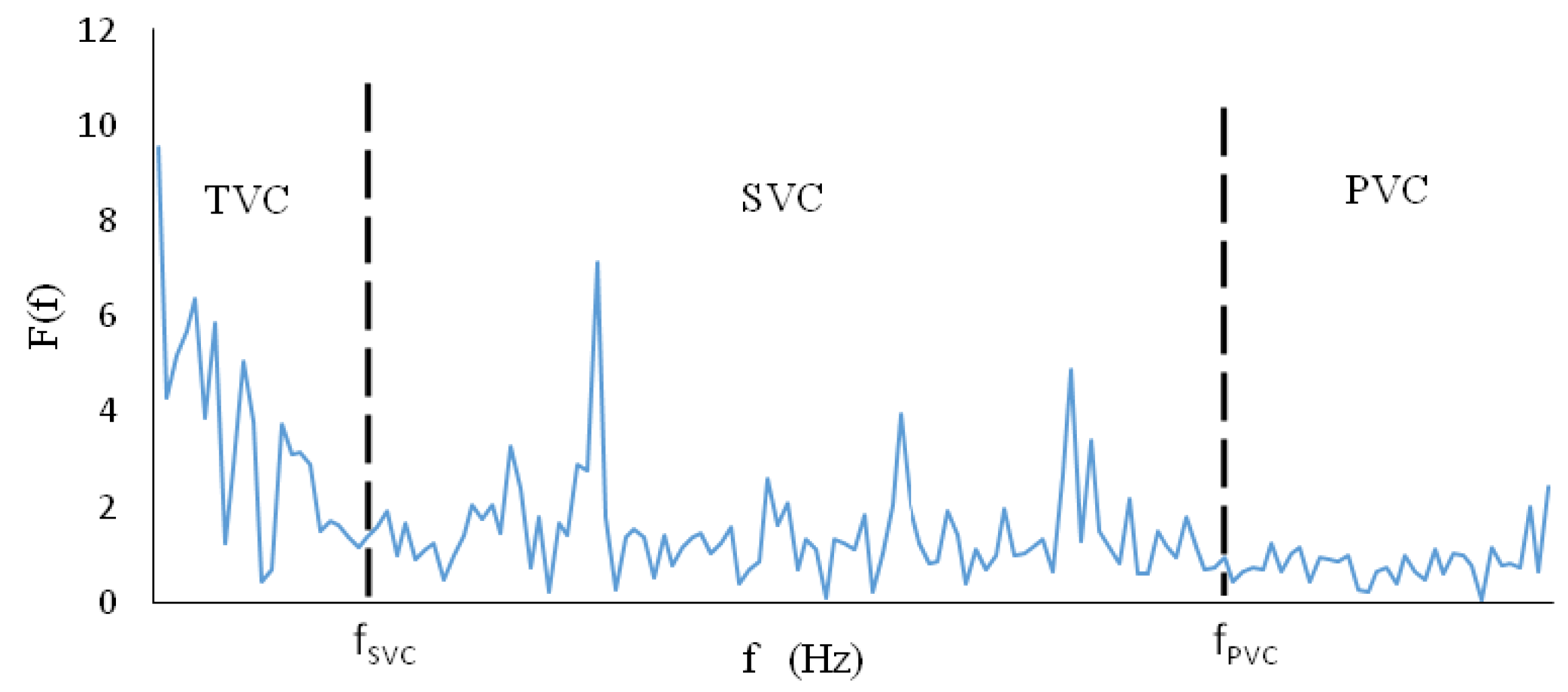
The historical reactive load demand data consists of a series of non-periodic discrete data containing a wide range of frequency components. As the main focus of this paper is SVC, we applied a band-pass filter to the load data. The pass band of the filter was (f_SVC, f_PVC), where f_SVC = 1/T_SVC and f_PVC = 1/T_PVC. However, the sampling frequency was limited for some of the data, and so the maximum valid frequency f_MAX was smaller than f_PVC. In this case, the pass band was set to (f_SVC, f_MAX). By processing the original data, we may obtain the mid-frequency component of the total load fluctuations, Q_SVC. We analyzed Q_SVC using a Fourier transform method as follows [20]:

$$Q_{\text{SVC}}\left(t\right)=\frac{1}{2\pi }{\int }_{-{\mathrm{\omega }}_{\text{PVC}}}^{-{\mathrm{\omega }}_{\text{SVC}}}F(\mathrm{\omega })e^{\text{j}\mathrm{\omega }t}d\mathrm{\omega }+\frac{1}{2\pi }{\int }_{{\mathrm{\omega }}_{\text{SVC}}}^{{\mathrm{\omega }}_{\text{PVC}}}F(\mathrm{\omega })e^{\text{j}\mathrm{\omega }t}d\mathrm{\omega }$$

(2)

The reactive power variations can be considered to be proportional to time in the case of very short time intervals. The differential form of Equation (2) is:

$$\frac{\mathrm{\Delta }{Q}_{\text{SVC}}(\text{t})}{\mathrm{\Delta }t}=\frac{1}{2\pi }\left({\int }_{-{\mathrm{\omega }}_{\text{PVC}}}^{-{\mathrm{\omega }}_{\text{SVC}}}\text{j}\mathrm{\omega }F(\mathrm{\omega })e^{\text{j}\mathrm{\omega }t}d\mathrm{\omega }+{\int }_{{\mathrm{\omega }}_{\text{SVC}}}^{{\mathrm{\omega }}_{\text{PVC}}}j\mathrm{\omega }F(\mathrm{\omega })e^{\text{j}\mathrm{\omega }t}d\mathrm{\omega }\right)$$

(3)

where the expression on the left-hand side of the equation contains the differential coefficient of Q_SVC(t), which indicates the rate of the reactive power change and describes the intensity of the reactive power fluctuation. Larger differential coefficients indicate more drastic fluctuations.

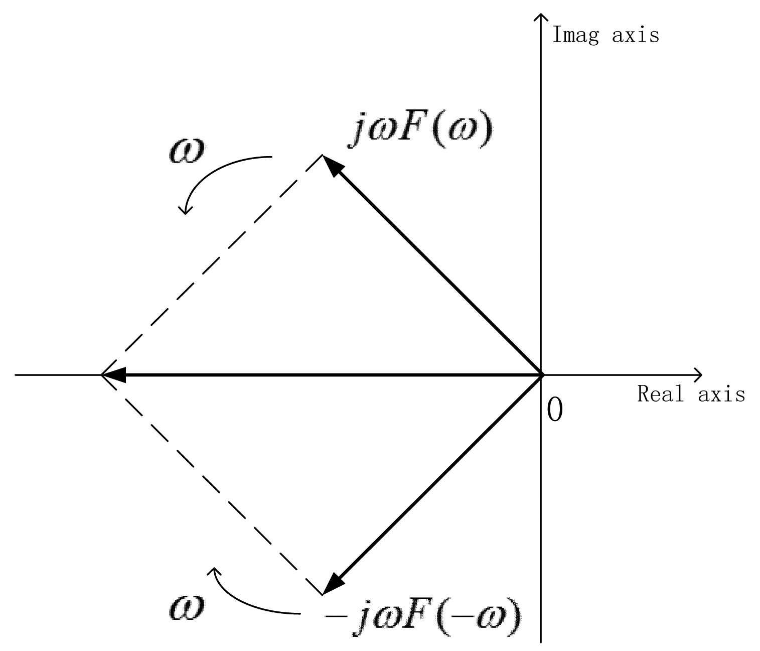
The differential coefficient is composed of a series of rotating phasors, e^jωt, the frequencies of which vary continuously from f_SVC to f_PVC (and from −f_PVC to −f_SVC). The magnitude of each phasor is. |F(f)|. F(f) and F(−f) are a pair of complex conjugates and rotate in the opposite directions with the same frequency. Figure 2 shows that the two phasors rotating at frequency 2πω can be synthesized into a phasor with an angle that does not change and magnitude that changes repeatly. Its maximum magnitude is 2ω|F(ω)|.

The Q-Fluctuation (QF) can be defined as:

$$QF=\frac{1}{\pi }{\int }_{{\mathrm{\omega }}_{\text{SVC}}}^{{\mathrm{\omega }}_{\text{PVC}}}\mathrm{\omega }\left|F(\mathrm{\omega })\right|d\mathrm{\omega }$$

(4)

The value of QF indicates the maximum magnitude of the differential coefficients of the reactive power. QF is the sum of the maximum magnitude of the synthesized phasor at each frequency; however, it should be noted that the possibility that all the phasors are a maximum at the same time is very small. The dimensions of QF and ΔQ/Δt are kvar·s⁻¹.

It should be noted that QF may be composed of several dominant components. Therefore, it is not necessary to use the integral form to express QF; instead, we can express it in the form of the sum of dominant components:

$$QF=\frac{1}{\pi }\sum _{i=1}^d\mathrm{\omega }\left|F\left(\mathrm{\omega }\right)\right|$$

(5)

where d is the number of the dominant components. There may be significant differences between different loads in terms of the number of dominant components and the frequencies of those components.

QF quantifies the load characteristic in terms of reactive power variation which lead to the voltage deviation. From Equation (5), there are two main elements: the angular velocity ω and the magnitude of the power fluctuations |F(ω)|. Higher frequency disturbances to the load are more likely to bring instant reactive power steps, leading to an instantaneous jump in the voltage. Bigger magnitude disturbances to the load are more likely to lead to bigger voltage deviations. Using the QF index, we may describe the reactive power fluctuations. However, only analyzing the fluctuation characteristic is not sufficient to evaluate the voltage deviation of each node which is the real information source of SVC, another factor that impacts is topological structure of the grid. An appropriate approach of combining load characteristic and topological structure is necessary to assess average voltage deviation for pilot node selection.

In practical, historical data is required to calculate the index, which comes from RTUs or PMUs that have already been widely installed over the grid. We can directly gather the necessary information from the Energy Management System (EMS) or Wide Area Measurement System (WAMS). In this sense, there is no new investment or extra costs to implement the proposed method.

3. Pilot Node Selection

3.1. Definition of the Voltage Fluctuation Space

The purpose of SVC is to reduce the node voltage deviations from the set-point values in each zone. The voltage deviation at a given node is the result of the reactive power fluctuations of all the loads in the region, and depends on the power grid structure and the distribution of control sources, which are conventionally described by the Q–V sensitivity [21]. The Q–V sensitivity quantifies the influence on voltage caused by a unit Q injection, while QF index quantifies the magnitude of the fluctuations. By connecting these two indices together, we can describe the V–Q relationships while taking the injection characteristics into account.

Let the time constant of the SVC be T_SVC, and QF_j be the QF of node j. VF_ij is defined as:

$$V{F}_{ij}=\left|S_{ij}\right|\cdot Q{F}_j\cdot T_{\text{SVC}}\text{with}{S}_{\mathit{\text{ij}}}=\stackrel{\partial V_i}{}/\underset{\partial Q_j}{}$$

(6)

and has units of kV (as does ΔV). The value of VF_ij is the intensity of the voltage deviations caused by a given reactive power load. Voltage deviations caused by reactive power fluctuations at different loads are treated as independent, and are represented by orthogonal vectors in a linear space termed the voltage fluctuation space (VFS), which is used to describe the impact of all reactive power load fluctuations. Each load has its own vector, which can be expressed as:

$${\overrightarrow{v}}_i=[V{F}_{i1},V{F}_{i2},\cdots ,V{F}_{\mathit{\text{ii}}},\cdots ,V{F}_{\mathit{\text{im}}}]$$

(7)

For two nodes i [VF_i1, VF_i2, …, VF_im] and j [VF_j1, VF_j2, …, VF_jm], the distance D_ij in VFS is then defined as:

$$D_{ij}=\sqrt{{\left|V{F}_{i1}-V{F}_{j1}\right|}^2+\cdots +{\left|V{F}_{im}-V{F}_{jm}\right|}^2}$$

(8)

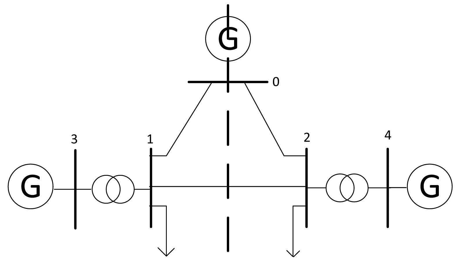
v⃗_i contains a comprehensive description of the node voltage deviations. Each coordinate VF_ij represents the influence of load j on the voltage at node i. In general, VF_ij is not equal to VF_ij because the characteristics of load i and load j may be different. A simple example system is shown in Figure 3. This system consists of three generators and three load nodes with bus 0 as the slack bus. This system is symmetrical, so ∂V₁/∂Q₂ is equal to ∂V₂/∂Q₁ and ∂V₁/∂Q₁ is equal to ∂V₂/∂Q₂. It is difficult to determine which node is more suitable for the pilot bus only from the structure information. Assume that the characteristics of load 1 and load 2 are very different; then, v⃗₁ and v⃗₂ are also very different. We will use this difference to choose the pilot bus.

3.2. Pilot Node Selection Method

In the traditional SVC, one node will be selected as a pilot bus in each zone. In the VFS, each node has a vector v⃗_i that describes the voltage deviations and they are the summations of V_ij. The index L_i that denotes the intensity of the voltage deviations is defined as:

$$L_i=\sum _{j=1}^{l}V{F}_{ij}$$

(9)

where i is the node number. The pilot node should be the one with the largest L_i, since larger L_i values indicate larger voltage deviations. We choose the most volatile node as the pilot bus so as to monitor the system load fluctuations more accurately and restrain the voltage deviation at a reasonable range.

Since we have chosen the most volatile load node as the pilot node, when a fault occurs in the power system leading to structural changes of the grid, this selection scheme will ensure the maximum effectiveness of the control system.

In practical use, the appropriate number of pilot nodes is usually more than one. In this condition, the node with the biggest L_i is selected as the first pilot bus. Second, other nodes that are most closely coupled with this pilot bus (the distance between them in VFS is less than a given threshold) will be marked. Then, such a process will be carried out recursively within the remained unmarked nodes to find the next pilot bus until all the nodes in this zone are marked.

3.3. Algorithm

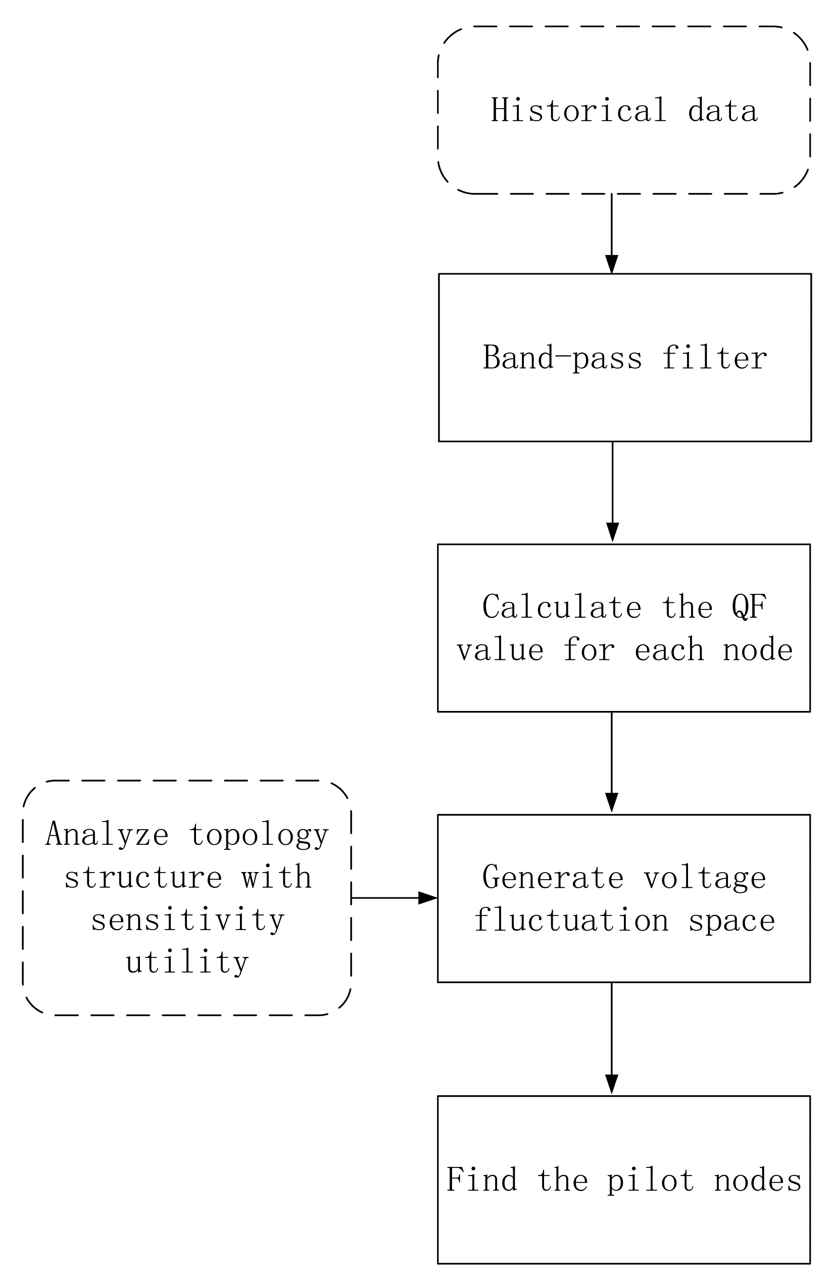
Figure 4 shows a flowchart describing the pilot selection method, which can be summarized as follows:

• Given the historical data of the reactive power for every load in the system, which contains load characteristic information;

• Apply a band-pass filter to restrict the data to frequency components within our range of interest;

• Fourier transform the historical data and calculate the QF values for each load using Equations (4) and (5);

• Generate the VFS based on the QF data and Q–V sensitivities using Equation (7);

• Calculate L_i for each node using Equation (9), and select the node with the proposed method.

4. Simulation Results

The IEEE 14-bus and 118-bus systems were used to investigate the performance of our method of pilot node selection.

4.1. IEEE 14-Bus System

The IEEE 14-bus system consists of five generators, nine loads, and 20 branches. For convenience of calculation and expression, the node numbering was modified. The structure of the system is shown in Figure 5. The slack bus, voltage-controlled buses (PV buses), and load buses (PQ buses) were as follows:

• Slack bus: Bus 14;

• PV buses: Buses 10, 11, 12, 13;

• PQ buses: Buses 1, 2, 3, 4, 5, 6, 7, 8, 9.

4.1.1. Calculation of QF

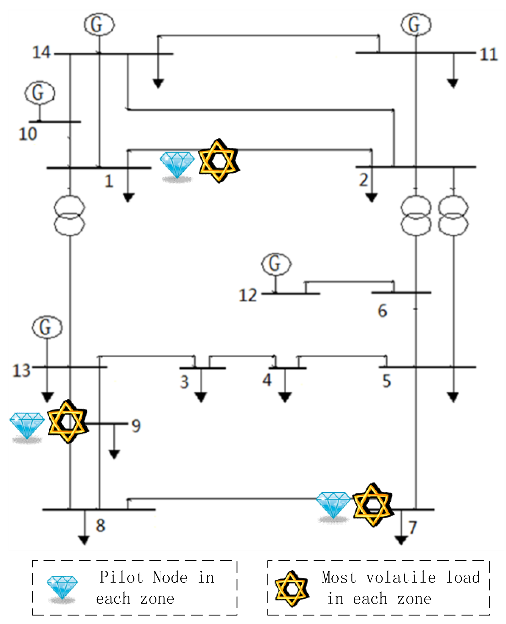
Nine sets of historical grid operating data were used as inputs to calculate QF at each load. Different types of loads were chosen to allow us to model different fluctuation characteristics. The QF values of loads 1, 7, and 9 were the largest; the position of these nodes is indicated in Figure 5 by the stars.

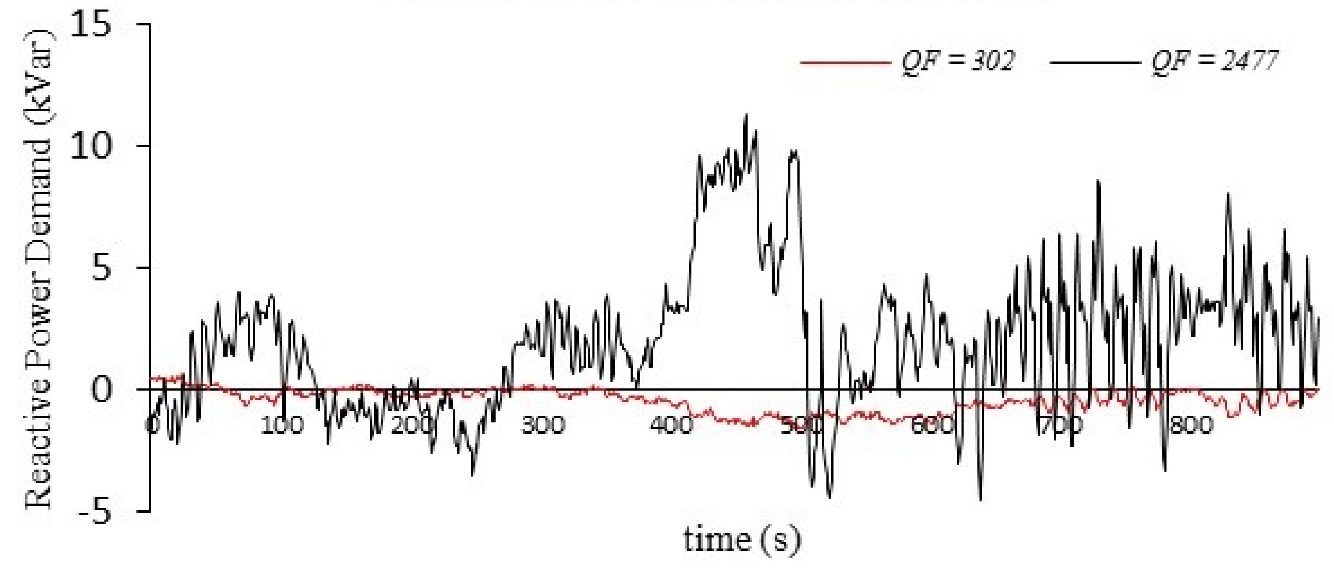
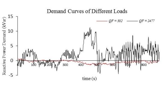
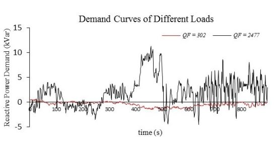
Here, we take two typical loads as an example to illustrate the concept of QF. Figure 6 shows two load–demand curves (of the nine); the QF values of the loads are also shown in the figure. The black curve, which corresponds to node 7, shows larger fluctuation than the red one, which corresponds to node 3. The QF values shown in the figure are also very different, with QF₇ is eight times of QF₃. The above results illustrate that QF is capable of representing the characteristic of load fluctuations.

4.1.2. Pilot Node Selection and Control Effect

To select the pilot node, first we must describe the system in the VFS. Since there were nine load nodes, the VFS had nine dimensions. There were three zones; we chose one node in each zone as the pilot node with the proposed method. The location of pilot nodes is marked with diamonds. The results of the system division and pilot node selection are as follows:

• Zone 1: nodes 1, 2, 10, 11; pilot node: 1;

• Zone 2: nodes 3, 4, 5, 6, 7, 12; pilot node: 7;

• Zone 3: nodes 8, 9, 13; pilot node: 9.

There were 84 ( $C_9^3$) scenarios of pilot node selection in all and total of them were simulated. The effectiveness of the voltage control with each pilot node selection for the same load fluctuations was compared. The disturbances were obtained from the historical operating data. The performance measure of the control used in this study can be expressed as the mean of the absolute voltage deviation at all load buses, i.e.,:

$$x=\frac{1}{m}\sum _{i=1}^m\left|x_i\right|$$

(10)

where m is the number of load buses in the test system and x_i (i = 1, 2, …, m) is the voltage change at each load bus.

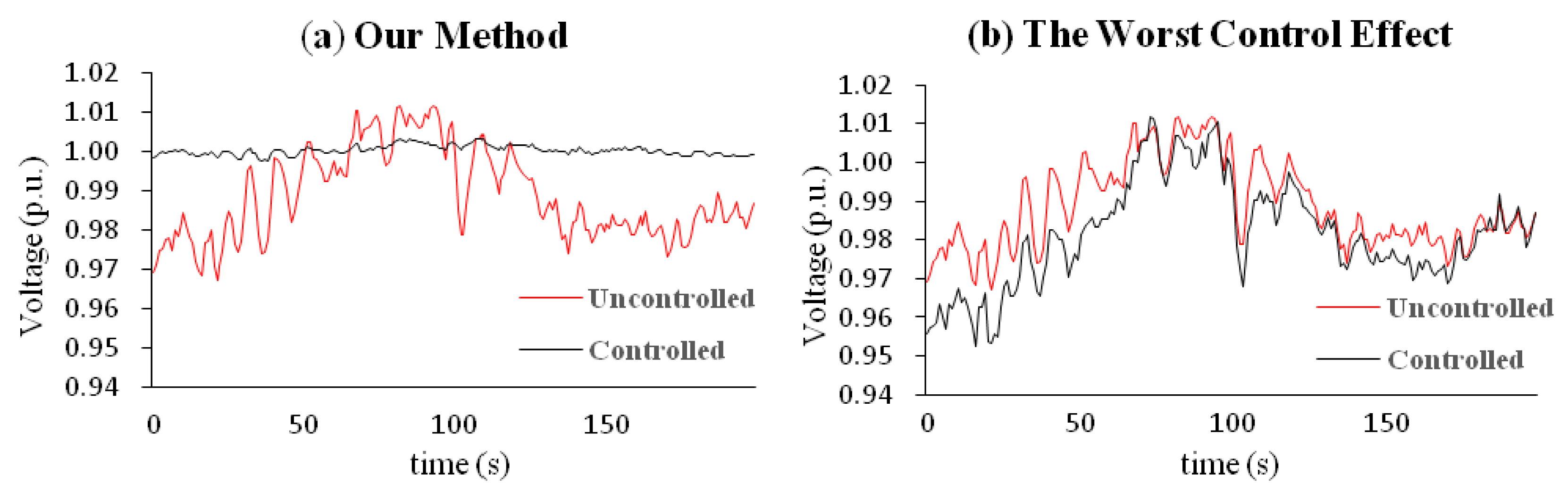
Simulation results are listed in

Table 1. Control effect of all the scenarios.

PMU location	Control result (p.u.)	PMU location	Control result (p.u.)
{1,2,3}	0.0163	{2,5,9}	0.0058
{1,2,4}	0.0198	{2,6,7}	0.0058
{1,2,5}	0.0036	{2,6,8}	0.0024
{1,2,6}	0.0042	{2,6,9}	0.0055
{1,2,7}	0.0032	{2,7,8}	0.0013
{1,2,8}	0.0114	{2,7,9}	0.0025
{1,2,9}	0.0155	{2,8,9}	0.0096
{1,3,4}	0.0073	{3,4,5}	0.0052
{1,3,5}	0.0042	{3,4,6}	0.0080
{1,3,6}	0.0047	{3,4,7}	0.0042
{1,3,7}	0.0073	{3,4,8}	0.0046
{1,3,8}	0.0036	{3,4,9}	0.0054
{1,3,9}	0.0080	{3,5,6}	0.0048
{1,4,5}	0.0042	{3,5,7}	0.0039
{1,4,6}	0.0080	{3,5,8}	0.0023
{1,4,7}	0.0013	{3,5,9}	0.0051
{1,4,8}	0.0036	{3,6,7}	0.0028
{1,4,9}	0.0099	{3,6,8}	0.0042
{1,5,6}	0.0035	{3,6,9}	0.0033
{1,5,7}	0.0028	{3,7,8}	0.0022
{1,5,8}	0.0048	{3,7,9}	0.0047
{1,5,9}	0.004	{3,8,9}	0.0061
{1,6,7}	0.0022	{4,5,6}	0.0055
{1,6,8}	0.0032	{4,5,7}	0.0068
{1,6,9}	0.0041	{4,5,8}	0.0036
{1,7,8}	0.0045	{4,5,9}	0.0052
{1,7,9}	0.0010	{4,6,7}	0.0018
{1,8,9}	0.0095	{4,6,8}	0.0053
{2,3,4}	0.0048	{4,6,9}	0.0089
{2,3,5}	0.0048	{4,7,8}	0.0041
{2,3,6}	0.0052	{4,7,9}	0.0017
{2,3,7}	0.0067	{4,8,9}	0.0046
{2,3,8}	0.0044	{5,6,7}	0.0040
{2,3,9}	0.0080	{5,6,8}	0.0034
{2,4,5}	0.0048	{5,6,9}	0.0055
{2,4,6}	0.0083	{5,7,8}	0.0072
{2,4,7}	0.0014	{5,7,9}	0.0023
{2,4,8}	0.0032	{5,8,9}	0.0040
{2,4,9}	0.0087	{6,7,8}	0.0053
{2,5,6}	0.0039	{6,7,9}	0.0025
{2,5,7}	0.0032	{6,8,9}	0.0031
{2,5,8}	0.0040	{7,8,9}	0.0025

. Among all these 84 methods, the scenario that we obtained by the proposed method achieved the best control result (marked with blue in Table 1). Figure 7 shows the best (x = 0.0010 p.u.) and worst (x = 0.0198 p.u.) control effect in the system. The proposed method was qualified to provide an optimal scenario in achieving satisfactory control effectiveness. Even though the grid, the fluctuations, and the control strategies were the same, the choice of the pilot nodes had a significant effect on the results of the SVC. Appropriate selection of the pilot nodes helped the SVC to inhibit voltage fluctuations; an inappropriate choice may result in worse system behavior than the uncontrolled situation.

4.1.3. Reliability Enhancement

Another advantage of our method is that it can enhance the reliability of the SVC in response to structural changes. Here, we compare the effectiveness of the AVC of our method and conventional methods [9] when the structure of the grid changes. The selection schemes were as follows:

• Our method: nodes 1, 7, and 9;

• Conventional method: nodes 1, 5, and 8.

There are 20 branches in the IEEE 14-Bus system. We assumed that one of the branches has an open circuit fault and that the topology of the grid changes. However, the load characteristics do not change. The control effectiveness of the SVC in five of the simulated cases are listed in

Table 2. Control effect of each fault condition.

Condition	Fault line		Control effect
	Start Node	End Node	Our method (p.u.)	Conventional method (p.u.)
1	13	1	0.0038	0.0041
2	6	2	0.0020	0.0046
3	5	2	0.0022	0.0071
4	5	4	0.0043	0.0070
5	4	3	0.0063	0.0045
Average value			0.0057	0.0063

, where the data listed describe the deviation from the set-point voltage and are expressed using the per-unit system.

The effectiveness of our control method was better than that of the conventional method in most cases. Appropriate pilot node selection is strongly related to the load characteristics. Even though the grid topology changed, the optimal pilot node selection does not necessarily also change. Our method is capable of enhancing the reliability of the control system in response to structural changes of the grid.

4.2. IEEE 118-Bus System

In this section, we simulate the IEEE 118-bus system.

4.2.1. System Division and Load Placement

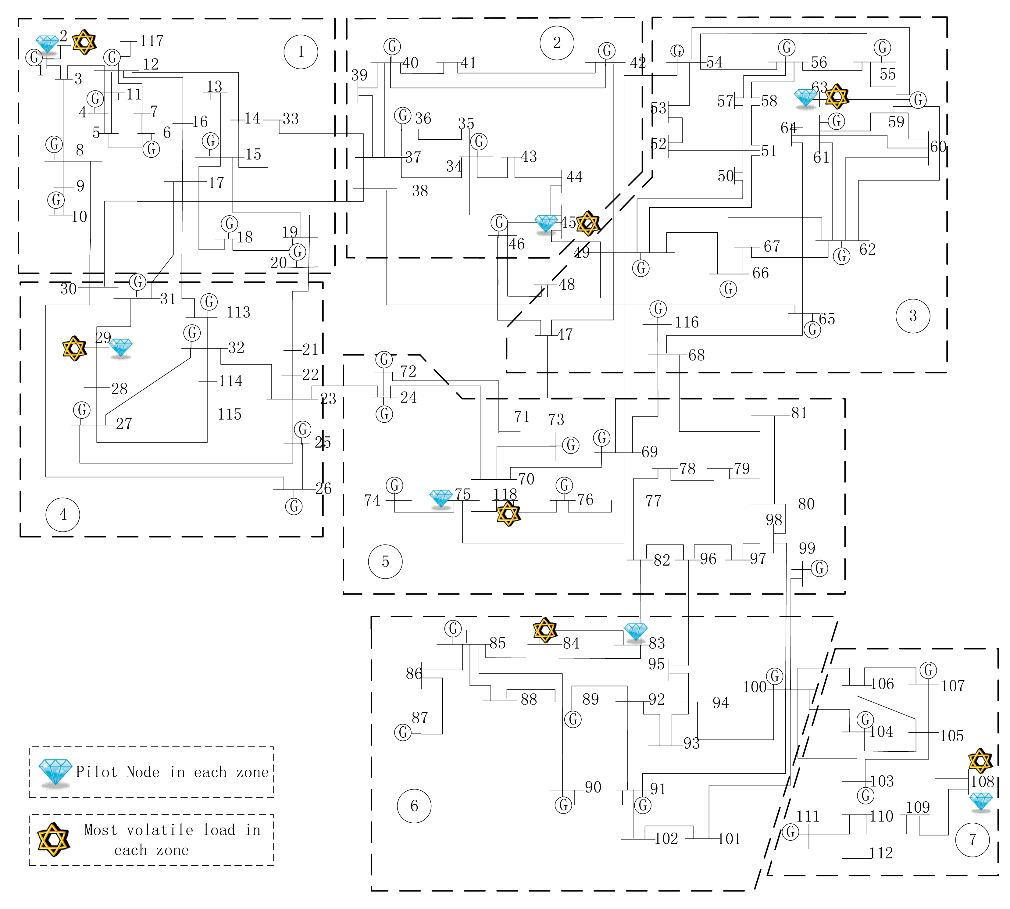
We used the system partition scheme described in [6] to partition the system into seven zones, as shown in Figure 8. The load with the largest QF was elaborately arranged in some relatively off-center nodes (marked with stars in the Figure). Conventional pilot node selection methods would not choose these off-center nodes as pilot nodes.

4.2.2. Pilot Node Selection

The results of the pilot node selection are listed in

Table 3. Simulation results for the IEEE 118-bus system.

Zone number	Pilot node	Control effect (p.u.)
		Our method	Best effect	Worst effect	Average
1	Node 2	0.0025	0.0021	0.016	0.0063
2	Node 45	0.0040	0.0040	0.0113	0.0087
3	Node 63	0.0032	0.0032	0.0059	0.0049
4	Node 29	0.0039	0.0036	0.0152	0.0079
5	Node 75	0.0002	0.0002	0.0073	0.0050
6	Node 83	0.0028	0.0028	0.0131	0.0093
7	Node 108	0.0015	0.0015	0.0023	0.0020

. The selected pilot nodes were all close to the most volatile loads (marked with diamonds in the Figure). In some zones, the pilot nodes were exactly where the most volatile loads were; for example, in zone 1, the pilot node and the most volatile load node were the same. This means that the reactive power of load 2 was the major source of system operation volatility. However, the pilot bus was not always the most volatile load. In zone 6, the most volatile load was node 84; however, node 83 was selected as the pilot node. This implies that the fluctuations of the surrounding loads had a significant impact on the voltage deviation of a given node.

4.2.3. Voltage Control

The effectiveness of the control method in each zone is listed in Table 3. In almost every zone, the selection method reported here resulted in superior effectiveness of the control system.

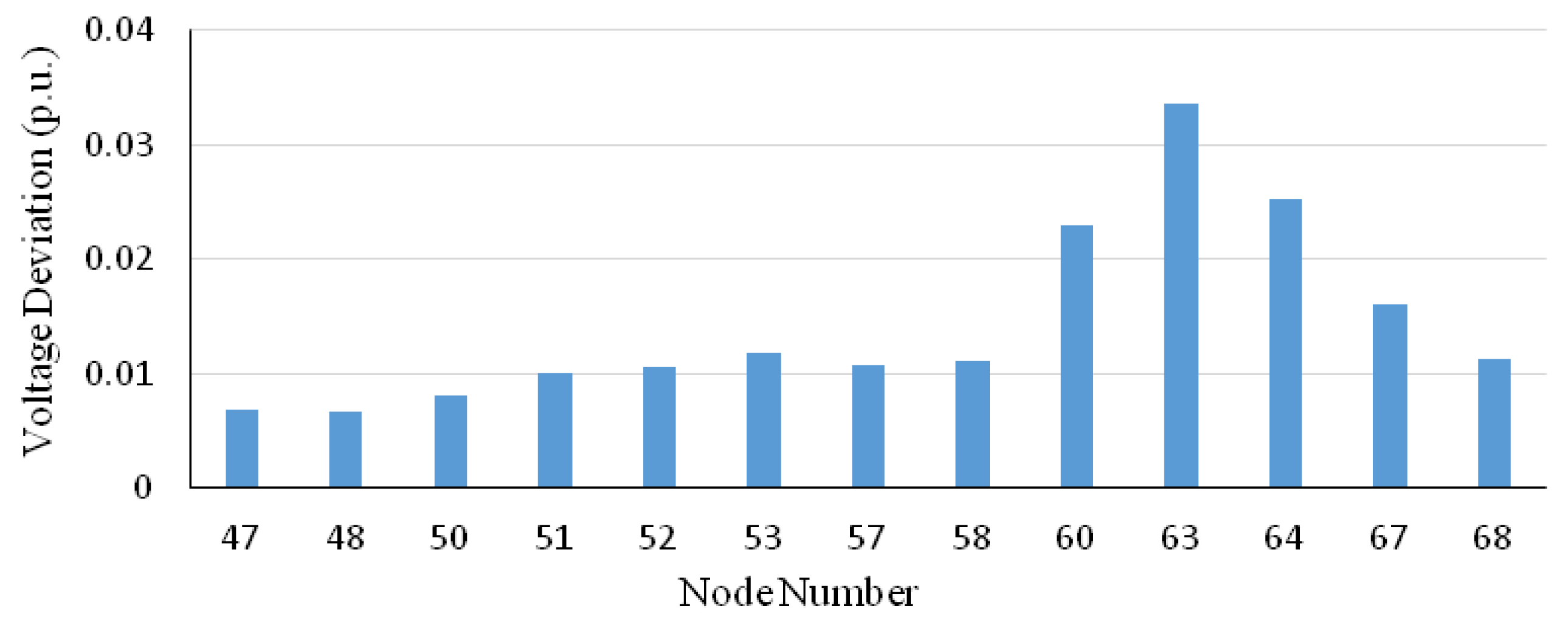
During SVC operation, the reactive power fluctuations at the loads in the system caused voltage deviations at all nodes. However, the impact on the different nodes was not equal. Figure 9 shows the voltage deviations at the different nodes in zone 3 when the fluctuations occurred. The voltage deviation at nodes 60, 63, and 64 were larger than at other nodes. This is why our method can help monitor the demand variations more accurately and with improved control.

The method described here may improve the observability of the system by way of adjusting the pilot bus selection without changing the information structure of the SVC. Historical data are used to define an impact factor to influence the decision. The analysis of historical data is essentially a simple forecast of the voltage deviation ΔV of each load. Therefore, this method expands the information structure of the SVC without requiring any additional observations.

5. Conclusions

We have described the concept of the QF index, which can be used to measure the characteristics of the reactive power demand fluctuations in terms of magnitude and frequency at the different nodes of a power system. Using the QF index, it is possible to take the load characteristics into account during the pilot node selection. We combined QF with the Q–V sensitivity of the power grid to define a VFS, which describes the average deviations of the voltage at each node. The operators of power systems will use this method to select more appropriate nodes as pilot nodes to take the load characteristics into account. In consequence, the performance of the SVC will be improved and the reliability of the control system will be enhanced.

The research of this method is based on the High-Voltage (HV) grids since we consider more about the hierarchical voltage control for transmission grids. Furthermore, large-scale wind powers are also integrated into the transmission grids in China. Compared with the HV grids, the common topological structure of Medium-Voltage (MV) and Low-Voltage (LV) grids are much simpler because most of them are radial. The coupling relationship is relatively simple. However, as more and more intermittent Distributed Generations (DGs) are being introduced into the distribution grids, the MV and LV grids are becoming much more complicated with possible loops and bigger fluctuations. Under the circumstances, the proposed method is also suitable for the MV and LV grids.

References

- Paul, J.P.; Leost, J.Y.; Tesseron, J.M. Survey of the secondary voltage control in France: Present realization and investigations. IEEE Power Eng. Rev. 1987, 7, 55–56. [Google Scholar]
- Guo, Q.; Su, H.; Zhang, M.; Tong, J.; Zhang, B.; Wang, B. Optimal voltage control of PJM smart transmission grid: Study, implementation, and evaluation. IEEE Trans. Smart Grid 2013, 4, 1665–1674. [Google Scholar]
- Corsi, S.; Pozzi, M.; Sabelli, C.; Serrani, A. The coordinated automatic voltage control of the Italian transmission grid—Part I: Reasons of the choice and overview of the consolidated hierarchical system. IEEE Trans. Power Syst. 2004, 19, 1723–1732. [Google Scholar]
- Ilic, M.D.; Liu, X.; Leung, G.; Athans, M.; Vialas, C.; Pruvot, P. Improved secondary and new tertiary voltage control. IEEE Trans. Power Syst. 1995, 10, 1851–1862. [Google Scholar]
- Hai, F.W.; Li, H.; Chen, H. Coordinated secondary voltage control to eliminate voltage violations in power system contingencies. IEEE Trans. Power Syst. 2003, 18, 588–595. [Google Scholar]
- Ilic-Spong, M.; Christensen, J.; Eichorn, K.L. Secondary voltage control using pilot point information. IEEE Trans. Power Syst. 1988, 3, 660–668. [Google Scholar]
- Lagonotte, P.; Sabonnadiere, J.C.; Leost, J.Y.; Paul, J.P. Structural analysis of the electrical system: Application to secondary voltage control in France. IEEE Trans. Power Syst. 1989, 4, 479–486. [Google Scholar]
- Guo, Q.; Sun, H.; Zhang, B.; Wu, W. Power network partitioning based on clustering analysis in mvar control space. Autom. Electr. Power Syst. 2005, 10, 36–40. [Google Scholar]
- Quintana, V.H.; Muller, N. Partitioning of power networks and applications to security control. IEE Proc. C Gener. Transm. Distrib. 1991, 138, 535–545. [Google Scholar]
- Yusof, S.B.; Rogers, G.J.; Alden, R.T.H. Slow coherency based network partitioning including load buses. IEEE Trans. Power Syst. 1993, 8, 1375–1382. [Google Scholar]
- Wang, Y.; Zhang, B.; Sun, H.; Niande, X. An expert knowledge based subarea division method for hierarchical and distributed electric power system voltage var optimization and control. Proc. CSEE 1998, 3, 221–224. [Google Scholar]
- Sun, H.; Guo, Q.; Zhang, B.; Wu, W.; Wang, B. An adaptive zone-division-based automatic voltage control system with applications in China. IEEE Trans. Power Syst. 2013, 28, 1816–1828. [Google Scholar]
- Conejo, A.; Gómez, T.; de la Fuente, J.I. Pilot-bus selection for secondary voltage control. Eur. Trans. Electr. Power 1993, 3, 359–366. [Google Scholar]
- Chen, R.; Guo, Q.; Sun, H. Pilot bus selection in automatic voltage control. Electr. Power Autom. Equip. 2012, 9, 111–116. [Google Scholar]
- Conejo, A.; Aguilar, M. A Nonlinear Approach to the Selection of Pilot Buses for Secondary Voltage Control. Proceedings of the Power System Control and Management Fourth International Conference, London, UK, April 1996; pp. 16–18.
- Conejo, A.; de la Fuente, J.I.; Goransson, S. Comparison of Alternative Algorithms to Select Pilot Buses for Secondary Voltage Control in Electric Power Networks. Proceedings of the Electrotechnical Conference, Antalya, Turkey, April 1994; pp. 12–14.
- Conejo, A.; Aguilar, M.J. Secondary voltage control: Nonlinear selection of pilot buses, design of an optimal control law, and simulation results. IEE Proc. Gener. Transm. Distrib. 1998, 145, 77–81. [Google Scholar]
- Su, H.Y.; Liu, C.W. An adaptive PMU-based secondary voltage control scheme. IEEE Trans. Smart Grid 2013, 4, 1514–1522. [Google Scholar]
- Zhijian, L.; Ilic, M.D. Toward PMU-Based Robust Automatic Voltage Control (AVC) and Automatic Flow Control (AFC). Proceedings of the Power and Energy Society General Meeting, Minneapolis, MN, USA, July 2010; pp. 25–29.
- Bracewell, R.N. The Fourier Transform and Its Applications; McGraw-Hill: New York, NY, USA, 1978. [Google Scholar]
- Sun, H.B.; Zhang, B.M. A systematic analytical method for quasi-steady-state sensitivity. Electr. Power Syst. Res. 2002, 63, 141–147. [Google Scholar]