Optimal Sizing of Battery Storage Systems for Industrial Applications when Uncertainties Exist


Abstract
: Demand response (DR) can be very useful for an industrial facility, since it allows noticeable reductions in the electricity bill due to the significant value of energy demand. Although most industrial processes have stringent constraints in terms of hourly active power, DR only becomes attractive when performed with the contemporaneous use of battery energy storage systems (BESSs). When this option is used, an optimal sizing of BESSs is desirable, because the investment costs can be significant. This paper deals with the optimal sizing of a BESS installed in an industrial facility to reduce electricity costs. A four-step procedure, based on Decision Theory, was used to obtain a good solution for the sizing problem, even when facing uncertainties; in fact, we think that the sizing procedure must properly take into account the unavoidable uncertainties introduced by the cost of electricity and the load demands of industrial facilities. Three approaches provided by Decision Theory were applied, and they were based on: (1) the minimization of expected cost; (2) the regret felt by the sizing engineer; and (3) a mix of (1) and (2). The numerical applications performed on an actual industrial facility provided evidence of the effectiveness of the proposed procedure.1. Introduction
It is well known that battery energy storage systems (BESSs), due to the number and variety of services they can provide, are powerful tools for the solution of some challenges that future micro grids will face [1–4]. Storage devices, in fact, are key components of micro grids, which are a cluster of loads and distributed resources optimally integrated and controlled in order to maximize technical and economic benefits [5]. The services BESS can provide can be enlarged further if optimal sizing and operation of BESSs are guaranteed.
Possible applications of BESSs that seem particularly useful are load leveling, reducing end-users' electricity bills, improving end-users' power quality and reliability, and spinning reserve [6,7].
In the frame of the above applications, we focused on the optimal sizing of a BESS installed in an industrial facility to reduce the facility's electricity bill. In the most general case, reducing the electricity bill can involve both energy [energy charge (EC)] and peak power (demand charge) [5,8]. This paper refers only to the EC, so reducing the electricity bill means only the ability of the end-user to increase its energy required from the grid during the lower price hours and decrease the energy required from the grid when the price is higher.
When sizing a BESS, a cost analysis should be conducted that takes into account investment costs, maintenance costs, and benefits associated with the installation of the BESS. These savings and benefits depend on the control strategy performed during the operation of the BESS. The optimal size of a BESS should be the size that can meet the anticipated needs at the minimum total cost.
However, to apply the sizing procedure for reducing the electricity bill, we must have some input data (“sizing framework”). In particular, the load demand of the industrial facility and the relationships that quantify the electricity bill, i.e., the way in which the electricity bill is calculated and the way in which it depends on electricity use at each time of day, must be known.
In defining the sizing framework, the engineer who is sizing the BESS (hereafter referred to as the “Decision Maker” or DM) can operate under the hypothesis of either a deterministic framework or under the uncertainty of the data associated with the problem. In the first case, which has been the more popular approach in the past, certain conditions are assumed and used as input data. In the second case, uncertainties are introduced and modeled probabilistically.
We contend that the problem of sizing storage systems to be installed to reduce the electricity bills of an industrial facility must be solved with uncertain data related to the problem. Our position is based on the fact that this is the only way the DM can properly include both short-term and long-term factors in the sizing procedure. Of course, future systems will be subject to random perturbations that unavoidably result in uncertainties in the sizing calculations. Thus, traditional, deterministic paradigms can lead to uneconomic or unreliable solutions.
Although sizing a BESS for an industrial facility is characterized by unavoidable uncertainties related to energy costs and loads, to the best knowledge of the authors, no papers have been published in the relevant literature dealing with the probabilistic sizing of battery storage systems to reduce facilities' electricity bills. However, some papers have addressed the probabilistic sizing of storage systems, but the systems were installed to reduce the uncertainties associated with wind power and photovoltaic power.
For example, with reference to wind power, in [9], a stand-alone system was considered, and the storage was calculated for different levels of mean load. In [10], dynamic sizing based on probabilistic forecasts and a real market situation was proposed, considering the degree of risk that a power producer would find acceptable. In [11,12], the possible smoothing effect of a BESS was simulated with an exponential moving average. In [13], a probabilistic reliability assessment method was proposed for determining the adequate size of an on-site energy storage system and determining the transmission upgrades required to connect wind generators' output power with the power system. In [14], a probabilistic method for sizing energy storage systems was proposed based on wind power forecast uncertainty; the proposed sizing methodology permitted the estimation of the size as a function of unserved energy.
With reference to photovoltaic power, in [15], a probabilistic approach was used to size both the PV system and the battery storage system for three selected sites in Italy, characterized by different values of solar radiation. In [16], a probabilistic approach for the design of a stand-alone hybrid generation system, including energy storage devices, was proposed, based on an index able to take into account the probability that loss of power supply occurs.
In this paper, the problem of sizing a BESS for reducing the end-user's electricity bill was solved by using a probabilistic approach based on a stepwise procedure, i.e., (1) a limited number of selected sizing alternatives for the BESS and of futures (i.e., possible values of uncertain input data) were chosen; (2) a probability was assigned for each future; (3) the total costs (investment cost, maintenance cost, and benefits) were calculated for each alternative and future (then, for each scenario—a particular alternative combined with a particular future, being an alternative a set of specified options and a future a set of specified uncertainties [10]); and (4) decision theory was used to obtain the best size for the BESS, taking into account the total costs and future probabilities. In particular, three approaches provided by decision theory were used, i.e., (1) the first was based on the minimization of expected cost; (2) the second was based on the regret felt by the DM; and (3) the third was based on a mix of (1) and (2). These approaches have been used extensively and successfully to solve several important planning problems associated with power systems [17–20].
Then, the original objectives of this paper were: (i) to propose a new method for sizing a BESS when uncertainties exist and (ii) to apply a decision theory-based process to obtain the best sizing alternative considering the various uncertainties involved in the sizing framework. The new method involves the solution of a constrained optimization model for the daily optimal operation of the battery with the aim of minimizing the total cost incurred for energy.
In this paper, we focused mainly on sizing BESSs for industrial applications. However, the proposed procedure can be extended easily to other types of end users, e.g., domestic and commercial loads.
The remainder of this paper is organized as follows: Section 2 formulates the BESS sizing problem and shows the procedure proposed for solving the problem; Section 3 presents the practical application of the proposed procedure to an actual industrial facility; our conclusions are presented in Section 4.
2. Problem Formulation and Solution Procedure
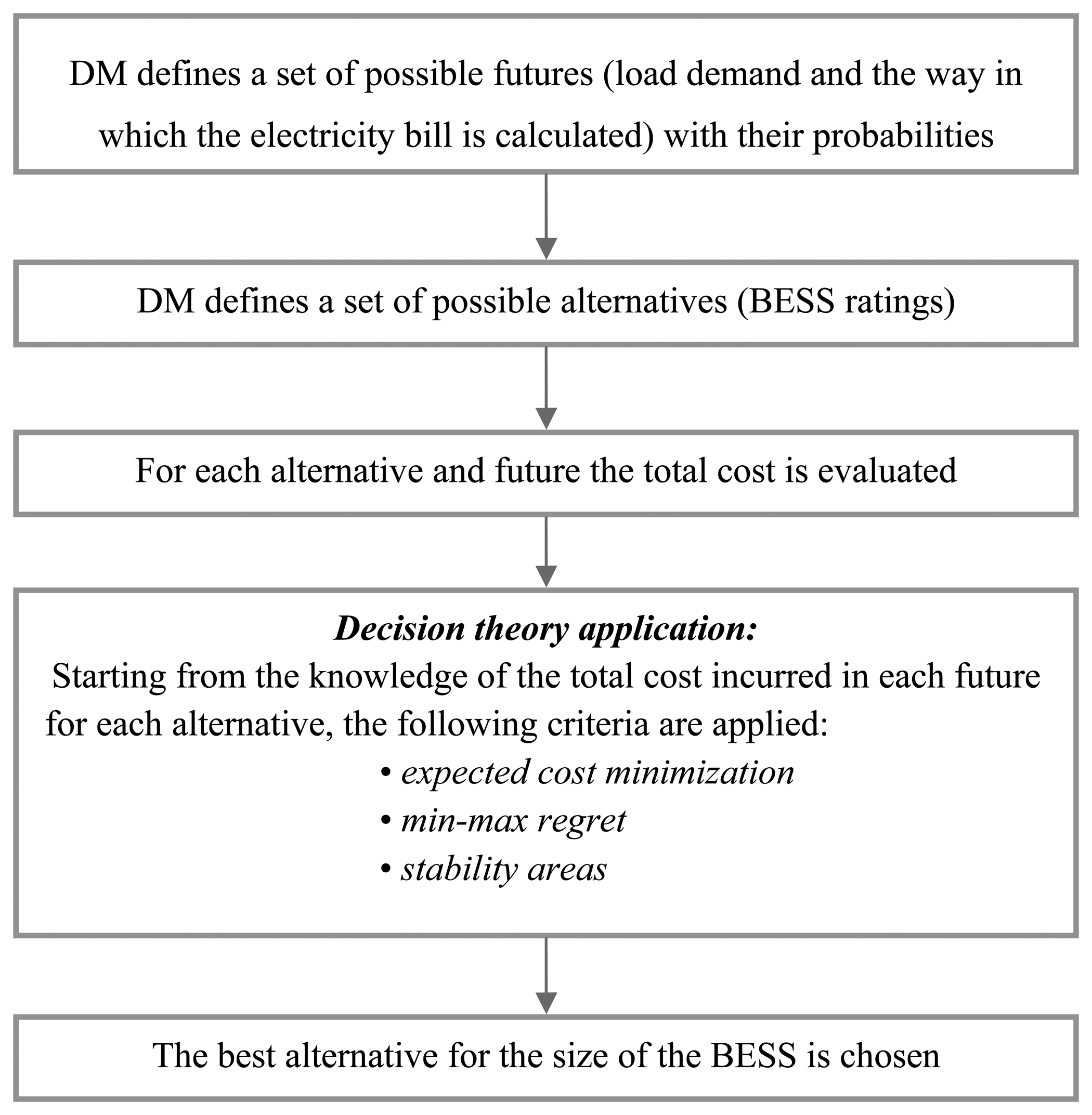
Let us consider an industrial facility's electrical distribution system in which one or more transformers connect the distribution grid to the lines of the users' power system. A BESS is connected at the secondary side of the transformers with the aim of reducing the electricity bill. We propose to solve the problem of BESS sizing under uncertainty with a four-step procedure, i.e.,
A set of possible futures is specified, and each future is characterized by a probability assigned by the DM. In this paper, each future is associated with a different industrial facility's load demand and the way in which the electricity bill is calculated, depending on electricity use at each time of the day.
Several possible BESS design alternatives are specified. Each design alternative is based on the BESS energy ratings, with its associated installation and maintenance costs.
The total BESS costs are calculated for each future specified in the first step and for each sizing alternative specified in the second step. The total costs take into account the installation cost, maintenance cost, and the benefits derived from the operation of the BESS. The benefits are obtained by solving an optimization problem in which the objective function to be minimized is the electricity bill and the constraints of which include the need to maximize the BESS's lifetime.
Decision theory is applied to choose, among the alternatives of the second step, the best BESS sizing solution by considering the futures with their probabilities, as specified in Step 1. The applied decision theory approaches used the future probabilities assigned in Step 1 and the total cost of the BESS calculated in Step 3; they are the minimization of the expected cost, the min-max regret, and the stability areas' criteria. These approaches have been used extensively and successfully for the solution of several important power system planning problems [17–20].
Figure 1 shows the flowchart of the proposed procedure.
We note that the DM, based on her or his understanding of the nature of the uncertainties relevant to the BESS sizing problem, selects possible alternatives and futures of Steps 1 and 2 and assigns the future probabilities [17–20]. We also note that three approaches usually are used to estimate the probabilities to be assigned when the future uncertainties are modeled probabilistically [17]:
- -
The first approach is based completely on the observed information.
- -
The second approach is based completely on the subjective judgment of the DM.
- -
The third approach is a mix of the above two approaches, and it combines the DM's judgmental information with the observed information.
In this paper, we used the second approach (subjective judgment of the DM). In fact, even if it may seem unsound to assign values of probabilities with little or no empirical information, surprisingly positive results can be obtained when the DM has a good understanding of the nature of the uncertainties relevant to the problem and uses this understanding to assign probabilities in a subjective manner [17–21].
In the next subsections, we show the details of the optimization problem to be solved in Step 3 and the decision theory criteria of Step 4.
2.1. Formulation of the Optimization Problem for Calculating the Total Costs for the BESS
As shown in Figure 1, the third step of the proposed procedure consists in calculating the total BESS costs for each future specified in the first step and for each sizing alternative specified in the second step.
Then, the aim of this subsection is to show how to calculate the total BESS cost. In the most general case, the calculation should be effected taking into account the investment costs, maintenance costs, and benefits derived from the installation of the BESS, that is:
While installation and maintenance costs depend on the BESS size, and as shown in [22], the maintenance cost is also a variable cost that is proportional to the size of the BESS and depends on the assumed lifetime of the BESS, the benefit derived from the use of storage depends also on the battery operation, that in this paper refers to the reduction of the electrical energy costs. This benefit can be evaluated through:
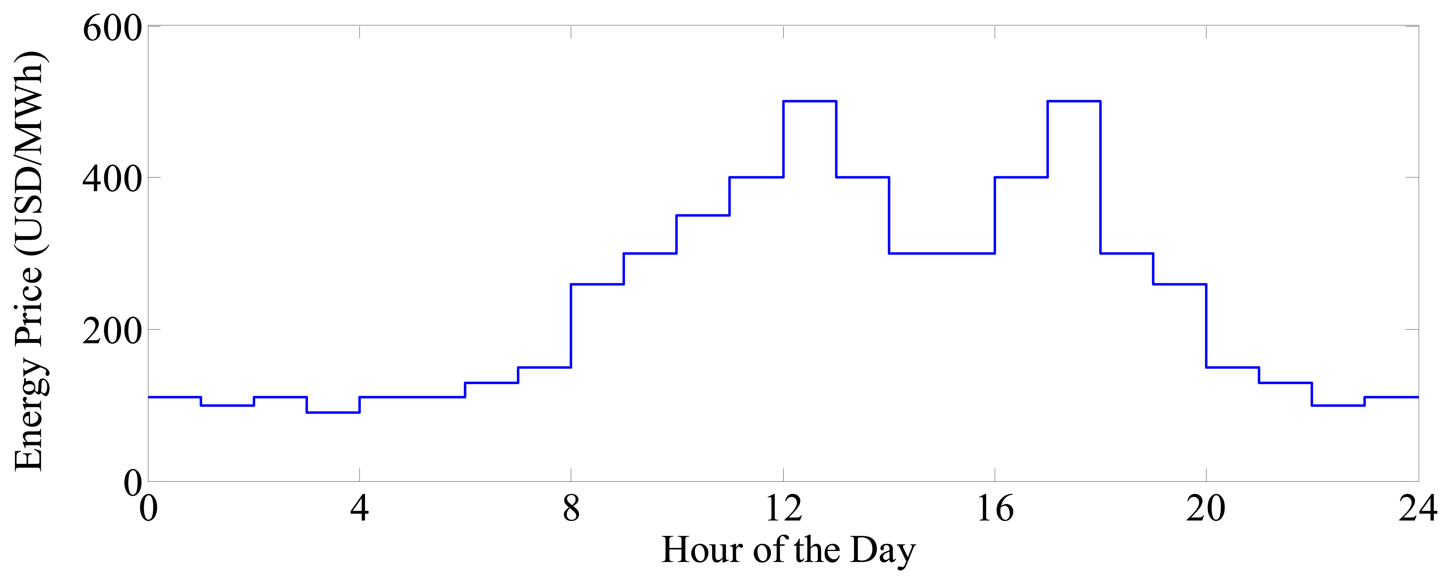
The BCwithB in Equation (3) can be calculated for 24 h (one day) [22], assuming as input data a typical daily profile of the industrial facility's load power and the hourly electricity price coefficients for the day. Also, more typical days can be considered, i.e., to cover weekly, monthly, and seasonal variations [23]. Once the typical daily electricity costs are known, they can be extended to cover the costs during the lifetime of the BESS to which this paper refers.
However, the evaluation of the daily cost is not an easy task, since, while the BESS operation is aimed at reduction of the electricity bill, at the same time technical constraints able to maximize the battery lifetime has to be met. In particular, constraints on the depth of discharge and the number of charging/discharging cycles per day have to be satisfied [4]. To do that, a control strategy based on a constrained optimization problem is needed. In this application, the procedure proposed in [8] is used. This procedure obtains the daily electricity bill with the BESS by solving an optimization problem such as:
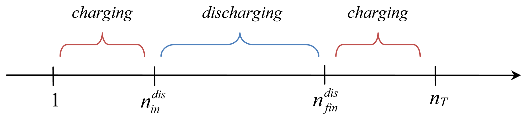
Before specifying the objective function and constraints in Equations (4) and (5), we outline that the optimization model refer to a day split into nT time intervals of length ΔTt and that, in order to limit one charging/discharging cycle, the day is separated into three intervals, as shown in Figure 2, with the first interval being the charging stage, the second interval being the discharging stage, and the third interval also referring to the charging stage. In this way, the condition of one cycle per day is clearly satisfied, because the last charging stage of the day continues with the first charging stage of the following day.
The time steps in which the discharging mode starts and ends ( , ) are optimization variables of the problem subjected to the constraint (and, obviously, bounded by 1 and nT). Based on the daytime steps of Figure 2, it is possible that the battery, at the beginning of the day, is either in charging mode (if or in discharging mode (if ); moreover, it is possible that, at the end of the day, the battery is either in charging mode (if or in discharging mode (if .
We outline also that we limited the BESS to only one charging/discharging cycle per day since its use can be profitable only if there is a large enough number of charging/discharging cycles to obtain significant economic benefits during the lifetime of the BESS. While a greater cost benefit could be obtained for a given day by multiple charging/discharging cycles, we must take into consideration the fact that operating in this manner ultimately decreases the lifetime of the BESS, producing an adverse effect on total cost. In our experience, the overall total cost benefits (i.e., the benefits obtained during the entire lifetime of the BESS) will be lower when multiple daily cycles are used than when only one daily charging/discharging cycle is used.
The objective function of the Equation (4) to be minimized is obviously the daily electricity bill, given by:
The first equality constraint in Equation (4) to be met refers to the power balance, and it requires that the total power value requested by the facility be equal to the sum of the BESS power and load demand power for all time intervals of the day:
Further equality constraints require that the daily balance of charging and discharging energy is satisfied:
Moreover, the inequality constraints require that the BESS can only charge during the charging period and only discharge otherwise:
It has to be highlighted that, during the lifetime of the battery, its features (e.g., efficiency, maximum storage capacity, and minimum storage capacity) vary with time based on the battery's aging characteristics [24]. Generally speaking, it could be possible to consider the effects of aging by dividing the planning problem into different time intervals, each one characterized by a specific set of storage properties (e.g., the battery's capacity or efficiency), depending on the aging effects versus time. However, to the best of our knowledge, this approach has never been used in the relevant literature in case of the BESS sizing; rather, the pertinent literature only takes into account the problem of the charging/discharging cycles, as was the case for our paper [4,5,22].
The above optimization model was solved with a hybrid approach based on a genetic algorithm (GA) and a linear optimization that operated inside the GA as an inner loop. The GA was used to obtain only the time intervals in which the BESS operates in the charging and discharging modes, while the linear optimization determined the state of charge of the BESS at the beginning of the day and the optimal charging/discharging powers of the BESS inside the above intervals to minimize the electricity bill cost function in Equation (6).
In more detail, the GA created populations in which the individuals referred to the times that the discharging mode started and ended ( , Figure 2). Once the GA has generated an individual and, hence, the charging and discharging intervals were unequivocally determined, the linear optimization algorithm solved the optimization problems in Equations (4) and (5).
When the inner linear optimization problem converges, the value assumed by the objective function in Equation (6) also represents the value of the fitness function related to each individual of the GA. The procedure terminates when the GA converges, i.e., when the best value of the fitness function remains constant over an assigned number of generations or when a maximum number of iterations is reached.
2.2. Decision Theory Criteria for the Choice of the Best Size for the BESS
As previously shown in Steps (1) and (2) of the proposed BESS sizing procedure, several futures are specified, with each future characterized by an assigned probability, and several design alternatives for the BESS are specified in terms of the energy to be produced by the BESS. In addition, in Step (3), for each future specified in the first step and for each alternative specified in the second step, the total cost of the BESS was calculated by optimizing the operation of the BESS.
Decision theory was used in Step 4 to choose, among the alternatives of Step 2, the best solution with respect to the size of the BESS by considering the futures with their probabilities as specified in step 1 and considering the total costs calculated in Step 3.
To choose the best solution, let the uncertainties in the sizing of the BESS be represented by a set of NF futures, Fk (k = 1, …, NF), with Pk being the future probability; each future is characterized by different values of the electricity cost coefficients ECt in Equation (6) and the profile of the load demandPL,t Let Na alternatives Ai (i = 1, …, Na) also be available, each corresponding to a different size of the BESS in term of energy production. Then, the problem of choosing the best solution must be solved. To solve the above problem, we apply three different decision theory approaches based on:
- (i)
minimizing the expected cost;
- (ii)
the regret felt by the DM;
- (iii)
a combination of (i) and (ii).
It should be noted that the application of decision theory requires knowledge of the total cost incurred in each future for each alternative. This has positively influenced the choice of the problem formulation in terms of a single-objective function in which the only objective is the total cost.
Approach (i) may be applied as follows. The expected value of the cost associated with all the NF futures can be calculated as:
Among all the possible alternatives, i.e., Ai (i = 1, …, Na), the alternative to be chosen is the one associated with the minimum value of the expected value of the cost:
The solution of the optimization problem in Equation (14) is Aopt, that is the alternative to be chosen. Basically, applying Approach (i) means that the DM choices the alternative that satisfies the mean of the futures that can occur. However, this choice does not avoid solutions that lead to bad performance in the future if an unfavorable future were to really occur. Basically, Approach (ii) tries to avoid such situations. In fact, minimizing the maximum regret means that the DM chooses the best solution among the worst solutions in order to avoid solutions that lead to a bad performance in the future [17–20].
In more detail, Approach (ii) indicates the best solution as the one that minimizes the regret felt by the DM after verifying that the decision he or she made was not optimal with respect to the future that actually occurred. The criterion is based on the calculation of the regret felt for having chosen a certain alternative Ai when the k-th future occurred; the regret is calculated as follows:
Finally, the sizing alternative, Aopt, to be chosen among the Na possible alternatives, is the one associated with the lowest value of Equation (17), i.e., the minimum of the maximum weighted regrets:
It should be noted that a critical aspect of both the above criteria (based on the expected cost and the regret) is the assignment of the probabilities Pk (k = 1, …, NF) that quantify the randomness of the sizing of the BESS, provided that both the expected costs and the weighted regrets depend on the probabilities. Several approaches for estimating these probabilities have been proposed [17], but none may fully overcome the probability assignment problem, either in the case of a high randomness or when the DM does not have a good understanding of the nature of the uncertainties relevant to the problem. Also, it can be useful to introduce a criterion based on the results of both procedures based on the DM's assessment.
In order to overcome the above problems, it may be convenient to refer to the “stability areas” concept proposed in [18]. Based on this concept, the scenario probabilities are treated as parameters that randomly vary in the range of [0, 1] while meeting the following constraint:
When the results of (i) and (ii) criteria are superimposed, the “stability area” of each sizing alternative is the area that corresponds to the probability for which both the Approaches (i) and (ii) give the same recommended solution for sizing the BESS. Based on the knowledge of all of the sizing alternatives characterized by a stability area different from zero (and of the corresponding area value), the DM can determine the sizing solution he or she considers to be the best. For example, the DM's final choice (i.e., the best size) could be the sizing alternative characterized by the greatest area, i.e., the one that appears most frequently as the best solution for both the Criteria (i) and (ii).
It should be also noted that assigning alternatives and futures is a further important aspect in the proposed approach. In the decision-making context, the DM identifies alternatives and futures on the basis of her/his understanding of the nature of the planning problem to be solved. In case of BESS sizing, these choices should be affected also considering: (i) that a maximum amount of investment cost can exist, imposed by the owner of the industrial facility; (ii) that there is a range of sizes within which the DM can forecast that the optimal solution will occur more frequently; and (iii) that the use of a very small number of futures can generate final decisions that will lead to bad performance in the future.
3. Experimental Section
The optimal procedure proposed in Section 2 was used to size a BESS to be connected to the secondary side of the transformer that connects an actual industrial facility to the medium voltage distribution grid. Among the batteries that are commercially available, either Li-ion or redox batteries can be used, both characterized by a long useful lifetime even with a significant depth of discharge [4,25]. We assumed a total value of $1,000/kW h for the investment and maintenance costs [4,22,26]; these costs include the controls and power conditioning system, and they take into account the forecasted decrease in the cost of the new generation electric battery [27]. A lifetime of about 4,500 cycles was assumed and it takes into account the forecasted increase in the lifetime of the new generation electric battery [26,27]. Then, having imposed one cycle per day, the period taken into consideration for the planning study is 12 years. The BESS is connected to the secondary side of the transformer by a pulse-width modulation controlled static converter. As is well known, the efficiency of the battery system depends on both the charge/discharge rate and the state of charge [28]; in this application, the charging efficiency was assumed to be 0.90, and the discharging efficiency was assumed to be 0.93 [4]. The maximum depth of discharge is 80%.
In order to better show the proposed sizing procedure, two different case studies are presented:
- -
Case 1: only three futures are considered (NF = 3); in this very simple case, the stability area criteria have a very simple graphical representation and, then, the proposed sizing approach can be more easily illustrated.
- -
Case 2: nine futures are considered (NF = 9).
With reference to the sizing alternative, 16 sizes for the BESS were considered (A1 = 0, A2 = 100, A3 = 200, A4 = 300, A5 = 400, A6 = 500, A7 = 600, A8 = 625, A9 = 650, A10 = 675, A11 = 700, A12 = 725, A13 = 750, A14 = 775, A15 = 800, A16 = 900 kW h). The sizing alternatives are chosen considering that: (i) a maximum amount of investment cost exists, imposed by the owner of the industrial facility, constraining the maximum value of the size to 900 kW h; and (ii) there is a range of sizes (between 600 kW h and 800 kW h) within which the DM forecasts that the optimal solution will occur more frequently, as will be shown later. Alternative A1 = 0 means that no BESS is installed.
3.1. Case 1
The following three futures were considered:
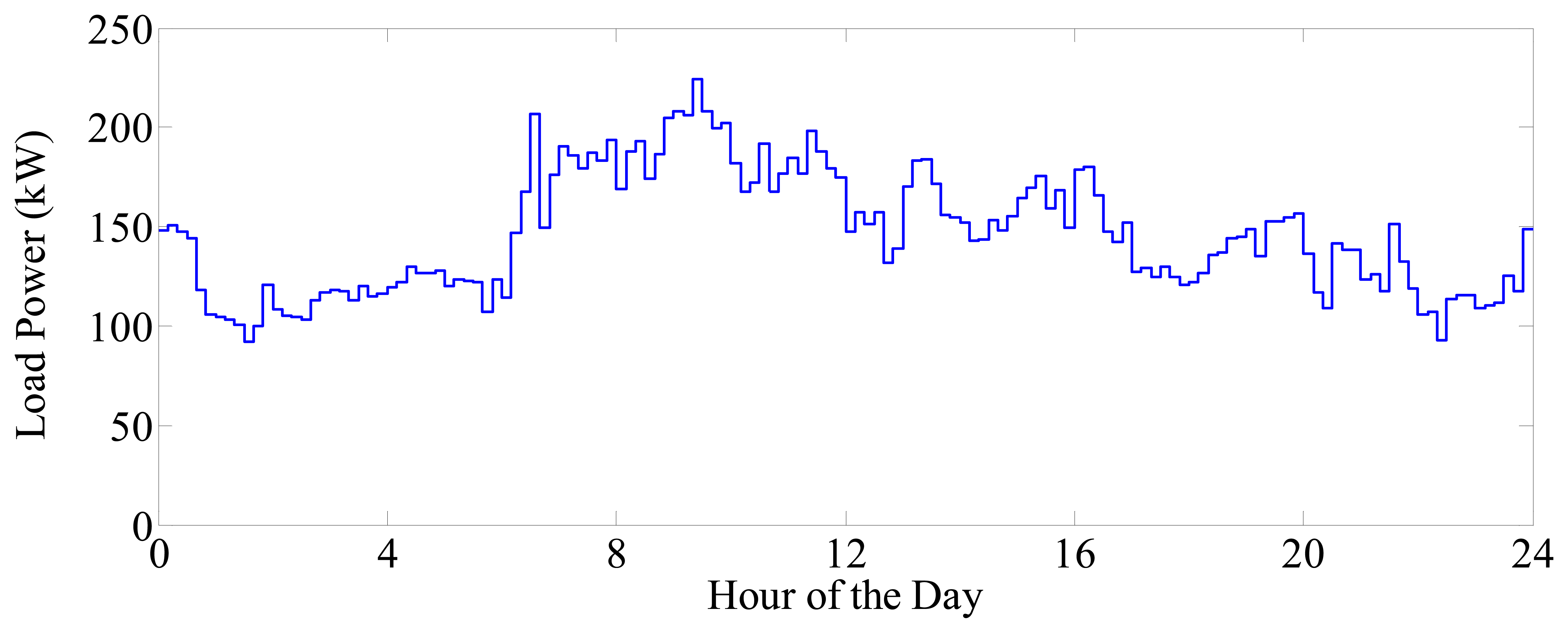
Future 1: the hourly EC profile reported in [22] for micro grids with storage system applications was assumed (Figure 3). The profile of the industrial facility's load demand was obtained by multiplying the profile in Figure 4 by 0.85.
Future 2: same as Future 1 except that the profile of the industrial facility's load demand was taken from Figure 4.
Future 3: same as Future 1, except that the profile of the industrial facility's load demand was obtained by multiplying the profile in Figure 4 by 1.15.
We considered three possible demand profiles, as suggested in [23]. The electricity costs were assumed to have a yearly rate of increase of 5%; a discount rate of 5% was assumed for the present value calculation.
Then, the three decision theory approaches were taken into account [approaches (i), (ii) and (iii) of Section 2.2]. For the application of the first two criteria, initially the following probabilities were assigned to each future, i.e., P1 = 0.2, P2 = 0.3, and P3 = 0.5.
Table 1 presents the decision matrix that shows each scenario that corresponds to the values of the total cost of the BESS (i.e., the sum of the energy bill and the investment/maintenance costs over the whole planning period); for each future, the minimum total cost is clearly marked.
From the analysis of the results in Table 1, it clearly appears that a slight variation of the load demand profile can generate a change in the size of the BESS that has the minimum cost (i.e., a 15% increase in the load profile generates the change from A7 to A9 and to A13 sizing alternatives, which are the optimal solutions for each future). Moreover, it is also interesting to observe that, for an assigned future, the total costs change slightly versus the size of the BESS, because the increasing values of the investment/maintenance costs for the BESS versus its size are compensated by the significant decreases in the electricity bill (i.e., by the increasing benefits derived from the installation of the BESS); as an example, in the case of the minimum cost sizing alternative, i.e., A9 = 650 kW h, the benefits derived from installing the BESS (i.e., the reduction of the electricity bill due to the availability of the BESS over the planning period) in the case of the load profile of Figure 4 (Future F2) are equal to $703,780 (18%).
Table 2 shows the decision matrix of the weighted regrets associated with each scenario; for each alternative, the maximum weighted regret is clearly marked. From the analysis of the results in Table 2, it clearly appears that the regret is equal to zero for the minimum total cost scenario.
Table 3 shows the expected value of the costs associated with the 16 alternatives and the maximum weighted regret calculated using the results in Table 2, and it should be noted that some slight numerical inaccuracies can arise in all Tables results due to digit truncation. From the analysis of the results in Table 3, it follows that the alternatives (BESS sizing) recommended by Approaches (i) and (ii) are slightly different, and they are given by A12 = 725 kW h and A11 = 700 kW h, respectively.
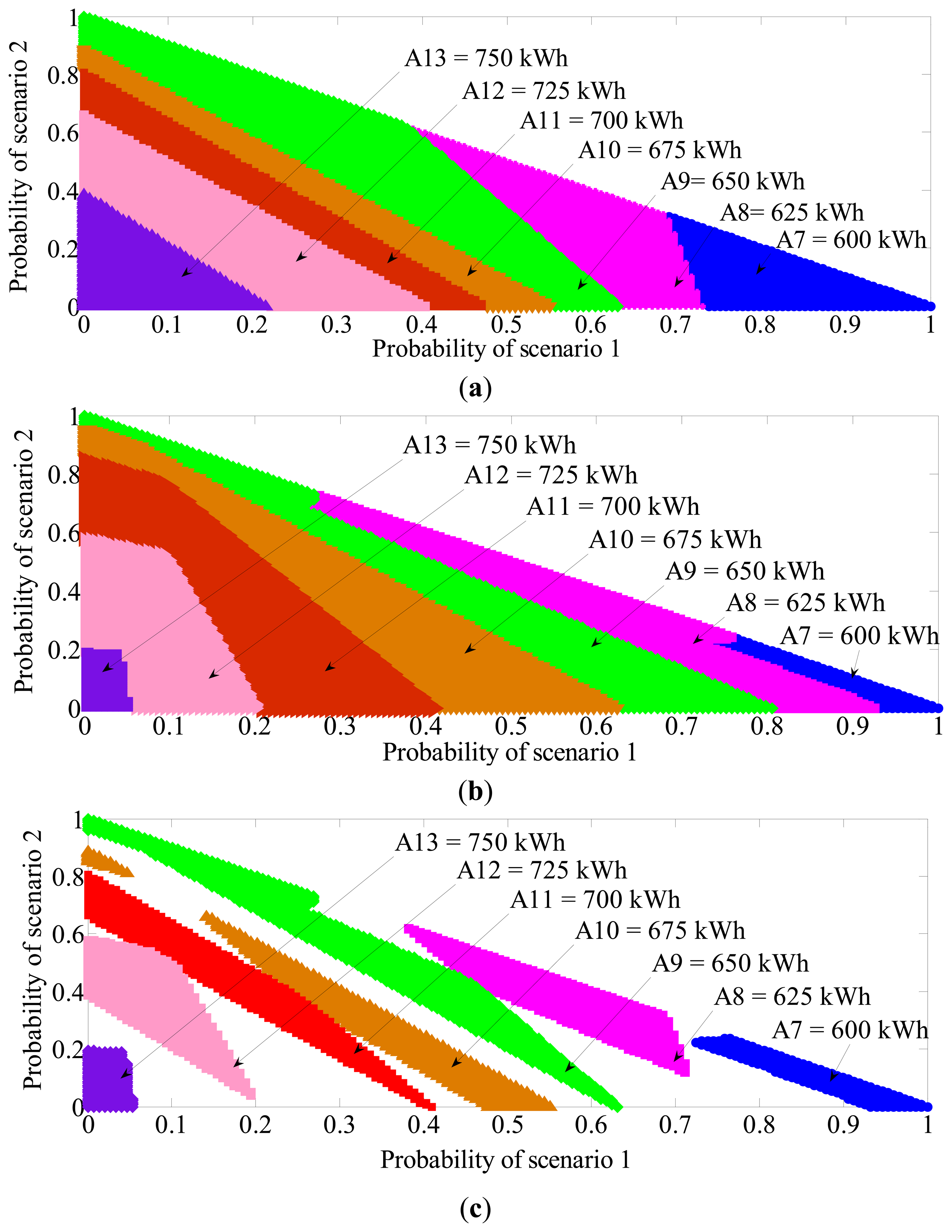
The stability areas for Approach (iii) (Figure 5c) were derived by superimposing those of Approaches (i) and (ii) (Figure 5a,b). To do that, many sets of three values of probabilities were generated randomly by varying P1, P2 and P3 while meeting Equation (19). Approaches (i) and (ii) were applied separately for each set of probabilities, and the sets were evaluated to identify and choose the optimal sizing alternative. Since it is trivial that P3 = 1 − P1 − P2 and an x-y plot is enough, a marker for each couple of probabilities P1, P2, the color of which distinguishes the optimal size obtained, is reported in Figure 5a [for Approach (i)] and Figure 5b [for Approach (ii)]. Then, overlapping the results of Approaches (i) and (ii), the stability areas were identified, thus obtaining Figure 5c, in which, for each couple of probabilities P1, P2, only the optimal solutions that contemporaneously satisfy both Approaches (i) and (ii) are shown with a marker, the color of which distinguishes the optimal size obtained. The white area corresponds to couples of probabilities that furnish different solutions when Approaches (i) and (ii) are applied.
The analysis of the stability area in Figure 5 provides the DM with a significant amount of information about the sizing process that can help her or him in the selection of the best size for the BESS.
Figure 5c shows that the alternative that occurs with the greatest frequency (area) is A9 = 650 kW h (about 12%). It is interesting to observe that both Approaches (i) and (ii) furnish seven sizing alternatives with varying future probabilities (Figure 5a,b). While the solution alternative suggested by Approach (iii), i.e., A9 = 650 kW h, was suggested most frequently, it is evident that other solutions were characterized by a significant stability area dimension; for example, about 9% of the trials gave the preferred solution as A11 = 700 kW h, and about 50% of trials presented different solutions with the same future probabilities (white area in Figure 5). Please note that all of the optimal sizing solutions are included between solution A7 = 600 kW h and solution A13 = 750 kW h, as forecasted by the DM.
It also is interesting to observe that the solutions in Figure 5 include the sizing alternatives when a deterministic future is assumed; for example, if the DM considers the future F1 to be the one that is actual occurring (i.e., the DM thinks Future 1 is a deterministic future), it follows that P1 = 1 and that P2 = P3 = 0. Then, from Figure 5a, the sizing alternative is A7 = 600 kW h, as is also evident from the analysis of Table 1 (first column).
In order to verify the effectiveness of the constraint of one cycle per day, some further simulations were performed by allowing more than one cycle. However, the results were that one cycle per day is always the optimal solution.
3.2. Case 2
The peak price and the gap between the minimum and maximum prices can have a strong influence on the benefits derived from the use of the BESS and, therefore, on the sizing of the BESS. Motivated by the above consideration, two price profiles were considered in addition to the profile in Figure 4: the first decreases in the peak price and in the gap between the minimum and maximum prices, while the second increases in the peak price and the gap between the minimum and maximum prices. Then, nine futures were considered that consisted of the combinations of the three profiles of the industrial facility's load requirements of Case 1 with the three profiles of the hourly ECs obtained by multiplying the values of Case 1 by 0.85, 1.0 and 1.15, respectively.
As an example, the following probabilities Pi at each scenario i are assigned: P1 = 0.1, P2 = 0.1, P3 = 0.1, P4 = 0.1, P5 = 0.1, P6 = 0.1, P7 = 0.2, P8 = 0.1 and P9 = 0.1 for the application of the first two criteria.
Table 4 reports the decision matrix, where, for each scenario, the corresponding values of the total cost of the BESS are shown.
From the analysis of the results in Table 4, it is interesting to observe that, when the energy cost coefficients are low (Futures 1, 4 and 7), the minimum cost solution is always A1 = 0 kW h (no BESS installation). In this case, the benefits due to the reduction of the electricity bill are not enough to justify the installation of the BESS; obviously, the same conclusion would arise if a reduction greater than 15% (i.e., 25% or 50%) was considered. On the contrary, when the energy cost coefficients are high (Futures 3, 6 and 9), the minimum cost solution is always A16 = 900 kW h (the maximum size of the BESS as constrained by the owner of the industrial facility).
Table 5 shows the decision matrix of the weighted regrets, and Table 6 shows the expected value of the costs associated with the 16 alternatives and the maximum weighted regret.
The effect of unequal probabilities is evident in Table 5, since Future F7 most heavily influences the weighted regrets, since P7 = 0.2 but all other probabilities are 0.1.
From the results in Table 6, it follows that, once again, the alternatives recommended by Approaches (i) and (ii) are different, and they are given by A9 = 650 kW h and A6 = 500 kW h, respectively. The stability areas for approach (iii) were derived by superimposing those of Approaches (i) and (ii). In this case, the stability area criterion cannot be represented with simple graphs as was done in Figure 5. The alternatives that resulted with a stability area different from zero were A6 = 500 kW h, A8 = 635 kW h, A9 = 650 kW h, A10 = 675 kW h, A12 = 725 kW h, A13 = 750 kW h, A14 = 775 kW h, A15 = 800 kW h, and A16 = 900 kW h. The sizing alternative with the greatest area was A13 = 750 kW h, followed by alternative A9 = 650 kW h.
As a final consideration on the sizing procedure, it should be noted that, even if the DM chooses a very high number of futures (much greater than nine) and if each optimization problem shown in the previous section is solved using GA and linear optimization, this does not result in excessive computational effort because the computations occur in the planning stage and new computers and configurations (parallel distributed processing and environment) can easily handle massive computational requirements.
4. Conclusions
This paper addressed the problem of determining the optimal size of a battery storage system to be installed in an industrial facility to reduce the facility's electricity bill. The main original contribution of the paper is that the sizing was conducted by using a probabilistic approach that took into account the unavoidable uncertainties involved with the electricity bill cost coefficients and the profile of the industrial facility's load demand. The choice of the optimal size for the BESS was made by using a stepwise procedure based on the application of decision theory. Different decision theory-based approaches were used, and the results were compared.
The main observations and outcomes of our analyses are that:
- -
The probabilities of the futures can significantly influence the optimal BESS sizing.
- -
The BESS optimal sizes obtained using the decision theory approaches involved various optimal sizing solutions with different stability areas, thus furnishing extensive and useful information for the DM's use in identifying the best solution.
- -
Decision theory appears to be a powerful tool in that it was able to solve the BESS sizing problem for industrial applications even when there were significant uncertainties, just as it has been for several other important problems associated with planning power systems.
As a final consideration, we stress that the slight differences in terms of cost and regret values for the assigned futures were not surprising. They were due to the high investment costs associated with an actual BESS that tend to mask their economic advantages. The future, worldwide-forecasted reduction in the investment costs associated with the installation of BESSs makes us confident that, in the near future, the economic advantages of BESS installations will be recognized and, consequently, there will be a pressing need for an optimal sizing procedure.
Future research will be devoted to the BESS sizing problem when the input data are treated as random variables characterized by their probability density functions; the results of that approach will be compared with the results obtained by assigning subjective probabilities and using decision theory, as we did in this paper. Future research also will consider other tariff schemes that involve both energy consumption (energy charge) and peak power (demand charge).
Acknowledgments
This paper is funded in the framework of the GREAT (GREAT: Research for Energy and Technology) Project supported by the GETRA Distribution Group (Italy).
Conflicts of Interest
The authors declare no conflict of interest.
References
- Manz, D.; Piwko, R.; Mille, N. Look before you leap: The role of energy storage in the grid. IEEE Power Energy Mag. 2012, 10, 75–84. [Google Scholar]
- Schroeder, A. Modeling storage and demand management in power distribution grids. Appl. Energy 2011, 88, 4700–4712. [Google Scholar]
- Ribeiro, P.F.; Johnson, B.K.; Crow, M.L.; Arsoy, A.; Liu, Y. Energy storage systems for advanced power applications. IEEE Proc. 2001, 89, 1744–1756. [Google Scholar]
- Divya, K.C.; Østergaard, J. Battery energy storage technology for power systems: An overview. Electr. Power Syst. Res. 2009, 79, 511–520. [Google Scholar]
- Johnson, M.P.; Bar-Noy, A.; Liu, O.; Feng, Y. Energy peak shaving with local storage. Sustain. Comput. Inform. Syst. 2011, 1, 177–188. [Google Scholar]
- Oudalov, A.; Chartouni, D.; Ohler, C.; Linhofer, G. Value Analysis of Battery Energy Storage Applications in Power Systems. Proceedings of the IEEE Power Systems Conference and Exposition (PSCE), Atlanta, GA, USA, 29 October–1 November 2006; pp. 2206–2211.
- Leou, R.C. An economic analysis model for the energy storage system applied to a distribution substation. Electr. Power Energy Syst. 2012, 34, 132–139. [Google Scholar]
- Carpinelli, G.; Khormali, S.; Mottola, F.; Proto, D. Optimal Operation of Electrical Energy Storage Systems for Industrial Applications. Proceedings of the IEEE Power and Energy Society General Meeting (PES), Vancouver, BC, Canada, 21–25 July 2013.
- Barton, J.P.; Infield, D.G. A probabilistic method for calculating the usefulness of a store with finite energy capacity for smoothing electricity generation from wind and solar power. J. Power Sources 2006, 162, 943–948. [Google Scholar]
- Pinson, P.; Papaefthymiou, G.; Klöckl, B.; Verboomen, J. Dynamic Sizing of Energy Storage for Hedging Wind Power Forecast Uncertainty. Proceedings of the IEEE Power & Energy Society General Meeting (PES), Calgary, AB, Canada, 26–30 July 2009.
- Paatero, J.V.; Lund, P.D. Effect of energy storage on variations in wind power. Wind Energy 2005, 8, 421–441. [Google Scholar]
- Koeppel, G.; Korpås, M. Improving the network infeed accuracy of non-dispatchable generators with energy storage devices. Electr. Power Syst. Res. 2008, 78, 2024–2036. [Google Scholar]
- Zhang, Y.; Songzhe, Z.; Chowdhury, A.A. Reliability modeling and control schemes of composite energy storage and wind generation system with adequate transmission upgrades. IEEE Trans. Sustain. Energy 2011, 2, 520–526. [Google Scholar]
- Bludszuweit, H.; Domínguez-Navarro, J.A. A probabilistic method for energy storage sizing based on wind power forecast uncertainty. IEEE Trans. Power Syst. 2011, 26, 1651–1663. [Google Scholar]
- Capizzi, G.; Bonanno, F.; Tina, G.M. Experiences on the Design of Stand-Alone Photovoltaic System by Deterministic and Probabilistic Methods. Proceedings of the International Conference on Clean Electrical Power (ICCEP), Ischia, Italy, 14–16 June 2011; pp. 328–335.
- Testa, A.; de Caro, S.; la Torre, R.; Scimone, T. Optimal Design of Energy Storage Systems for Stand-Alone Hybrid Wind/PV Generators. Proceedings of the International Symposium on Power Electronics Electrical Drives Automation and Motion (SPEEDAM), Pisa, Italy, 14–16 June 2010; pp. 1291–1296.
- Anders, G.J. Probability Concepts in Electric Power Systems; John Wiley & Sons: New York, NY, USA, 1990. [Google Scholar]
- Miranda, V.; Proenca, L.M. Why risk analysis outperforms probabilistic choice as the effective decision support paradigm for power system planning. IEEE Trans. Power Syst. 1998, 13, 643–648. [Google Scholar]
- Carpaneto, E.; Chicco, G.; Mancarella, P.; Russo, A. Cogeneration planning under uncertainty. Part II: Decision theory-based assessment of planning alternatives. Appl. Energy 2011, 88, 1075–1083. [Google Scholar]
- Carpinelli, G.; Celli, G.; Pilo, F.; Russo, A. Embedded generation planning under uncertainty including power quality issues. Eur. Trans. Electr. Power 2003, 13, 381–389. [Google Scholar]
- Carpinelli, G.; Ferruzzi, G.; Russo, A. Trade-off analysis to solve a probabilistic multi-objective problem for passive filtering system planning. Int. J. Emerg. Electr. Power Syst. 2013, 14, 275–284. [Google Scholar]
- Chen, S.X.; Gooi, H.B.; Wang, M.Q. Sizing of energy storage for microgrids. IEEE Trans. Smart Grid. 2012, 3, 142–151. [Google Scholar]
- Yahyaie, F.; Soong, T. Optimal Operation Strategy and Sizing of Battery Energy Storage Systems. Proceedings of the 25th IEEE Canadian Conference on Electrical and Computer Engineering (CCECE), Montreal, QC, Canada, 29 April–2 May 2012.
- Choi, S.S.; Lim, H.S. Factors that affect cycle-life and possible degradation mechanisms of a Li-ion cell based on LiCoO2. J. Power Sources 2002, 111, 130–136. [Google Scholar]
- Zaghib, K.; Dontigny, M.; Guerfi, A.; Charest, P.; Rodrigues, I.; Mauger, A.; Julien, C.M. Safe and fast-charging Li-ion battery with long shelf life for power applications. J. Power Sources 2011, 196, 3949–3954. [Google Scholar]
- Akhil, A.A.; Huff, G.; Currier, A.B.; Kaun, B.C.; Rastler, D.M.; Chen, S.B.; Cotter, A.L.; Bradshaw, D.T.; Gauntlett, W.D. DOE/EPRI 2013 Electricity Storage Handbook in Collaboration with NRECA; Sandia Report; Sandia National Laboratories: Albuquerque, NM, USA, 2013. [Google Scholar]
- United States Department of Energy. The Recovery Act: Transforming America's Transportation Sector—Batteries and Electrical Vehicles. 2010. Available online: http://bit.ly/fGaZPB (accessed on 11 December 2013).
- Johnson, V.H. Battery performance models in ADVISOR. J. Power Sources 2002, 110, 321–329. [Google Scholar]


| Alternative | Future | ||
|---|---|---|---|
| F1 | F2 | F3 | |
| A1 = 0 | 3,247.81 | 3,820.96 | 4,394.10 |
| A2 = 100 | 3,239.27 | 3,812.41 | 4,385.55 |
| A3 = 200 | 3,230.72 | 3,803.86 | 4,377.01 |
| A4 = 300 | 3,222.17 | 3,795.32 | 4,368.46 |
| A5 = 400 | 3,213.63 | 3,786.77 | 4,359.91 |
| A6 = 500 | 3,205.08 | 3,778.22 | 4,351.37 |
| A7 = 600 | 3,202.88 | 3,769.68 | 4,342.82 |
| A8 = 625 | 3,203.66 | 3,767.93 | 4,340.69 |
| A9 = 650 | 3,204.90 | 3,767.17 | 4,338.55 |
| A10 = 675 | 3,206.63 | 3,767.43 | 4,336.41 |
| A11 = 700 | 3,208.87 | 3,767.91 | 4,334.38 |
| A12 = 725 | 3,211.12 | 3,768.69 | 4,332.86 |
| A13 = 750 | 3,213.36 | 3,769.67 | 4,332.25 |
| A14 = 775 | 3,215.61 | 3,771.10 | 4,332.53 |
| A15 = 800 | 3,217.85 | 3,773.04 | 4,332.95 |
| A16 = 900 | 3,226.82 | 3,782.01 | 4,337.29 |
| Alternative | Future | ||
|---|---|---|---|
| F1 | F2 | F3 | |
| A1 = 0 | 8,986.37 | 16,136.42 | 30,925.44 |
| A2 = 100 | 7,277.12 | 13,572.58 | 26,652.42 |
| A3 = 200 | 5,567.90 | 11,008.74 | 22,379.36 |
| A4 = 300 | 3,858.67 | 8,444.89 | 18,106.28 |
| A5 = 400 | 2,149.46 | 5,881.05 | 13,833.20 |
| A6 = 500 | 440.23 | 3,317.21 | 9,560.14 |
| A7 = 600 | 0.00 | 753.37 | 5,287.08 |
| A8 = 625 | 156.69 | 229.75 | 4,218.80 |
| A9 = 650 | 404.63 | 0.00 | 3,150.52 |
| A10 = 675 | 750.22 | 79.57 | 2,082.28 |
| A11 = 700 | 1,198.92 | 222.81 | 1,064.98 |
| A12 = 725 | 1,647.61 | 457.85 | 307.48 |
| A13 = 750 | 2,096.30 | 751.09 | 0.00 |
| A14 = 775 | 2,545.00 | 1,179.10 | 139.41 |
| A15 = 800 | 2,993.69 | 1,760.41 | 348.65 |
| A16 = 900 | 4,788.46 | 4,452.57 | 2,522.22 |
| Alternative | E[C(Ai)] | |
|---|---|---|
| A1 = 0 | 3,992.90 | 30,925.44 |
| A2 = 100 | 3,984.35 | 26,652.42 |
| A3 = 200 | 3,975.81 | 22,379.36 |
| A4 = 300 | 3,967.26 | 18,106.28 |
| A5 = 400 | 3,958.71 | 13,833.20 |
| A6 = 500 | 3,950.17 | 9,560.14 |
| A7 = 600 | 3,942.89 | 5,287.08 |
| A8 = 625 | 3,941.46 | 4,218.80 |
| A9 = 650 | 3,940.41 | 3,150.52 |
| A10 = 675 | 3,939.76 | 2,082.28 |
| A11 = 700 | 3,939.34 | 1,198.92 |
| A12 = 725 | 3,939.26 | 1,647.61 |
| A13 = 750 | 3,939.70 | 2,096.30 |
| A14 = 775 | 3,940.71 | 2,545.00 |
| A15 = 800 | 3,941.95 | 2,993.69 |
| A16 = 900 | 3,948.61 | 4,788.46 |
| Alternative | Future | ||||||||
|---|---|---|---|---|---|---|---|---|---|
| F1 | F2 | F3 | F4 | F5 | F6 | F7 | F8 | F9 | |
| A1 = 0 | 2,760.64 | 3,247.81 | 3,767.98 | 3,247.81 | 3,820.96 | 4,394.10 | 3,734.98 | 4,394.10 | 5,053.21 |
| A2 = 100 | 2,768.37 | 3,239.27 | 3,710.16 | 3,255.55 | 3,812.41 | 4,369.27 | 3,742.72 | 4,385.55 | 5,028.39 |
| A3 = 200 | 2,776.11 | 3,230.72 | 3,685.33 | 3,263.28 | 3,803.86 | 4,344.44 | 3,750.46 | 4,377.01 | 5,003.56 |
| A4 = 300 | 2,783.84 | 3,222.17 | 3,660.50 | 3,271.02 | 3,795.32 | 4,319.62 | 3,758.19 | 4,368.46 | 4,978.73 |
| A5 = 400 | 2,791.58 | 3,213.63 | 3,635.67 | 3,278.76 | 3,786.77 | 4,294.79 | 3,765.93 | 4,359.91 | 4,953.90 |
| A6 = 500 | 2,799.31 | 3,205.08 | 3,610.84 | 3,286.49 | 3,778.23 | 4,269.96 | 3,773.66 | 4,351.37 | 4,929.07 |
| A7 = 600 | 2,812.44 | 3,202.88 | 3,593.31 | 3,294.23 | 3,769.68 | 4,245.13 | 3,781.40 | 4,342.82 | 4,904.25 |
| A8 = 625 | 2,816.86 | 3,203.66 | 3,590.46 | 3,296.49 | 3,767.93 | 4,239.37 | 3,783.33 | 4,340.69 | 4,898.04 |
| A9 = 650 | 2,821.66 | 3,204.90 | 3,588.14 | 3,299.59 | 3,767.17 | 4,234.74 | 3,785.27 | 4,338.55 | 4,891.83 |
| A10 = 675 | 2,826.88 | 3,206.63 | 3,586.14 | 3,303.57 | 3,767.43 | 4,231.30 | 3,787.20 | 4,336.41 | 4,885.62 |
| A11 = 700 | 2,832.54 | 3,208.88 | 3,585.21 | 3,307.72 | 3,767.91 | 4,228.10 | 3,789.22 | 4,334.38 | 4,879.54 |
| A12 = 725 | 2,838.20 | 3,211.12 | 3,584.04 | 3,312.14 | 3,768.69 | 4,225.25 | 3,791.68 | 4,332.86 | 4,874.04 |
| A13 = 750 | 2,843.86 | 3,213.36 | 3,582.87 | 3,316.72 | 3,769.67 | 4,222.62 | 3,794.91 | 4,332.25 | 4,869.59 |
| A14 = 775 | 2,849.52 | 3,215.61 | 3,581.70 | 3,321.68 | 3,771.10 | 4,220.51 | 3,798.90 | 4,332.53 | 4,866.16 |
| A15 = 800 | 2,855.17 | 3,217.85 | 3,580.53 | 3,327.08 | 3,773.04 | 4,218.99 | 3,803.00 | 4,332.95 | 4,862.89 |
| A16 = 900 | 2,877.80 | 3,226.82 | 3,575.85 | 3,349.71 | 3,782.01 | 4,214.31 | 3,821.70 | 4,337.29 | 4,852.89 |
| Alternative | Future | ||||||||
|---|---|---|---|---|---|---|---|---|---|
| F1 | F2 | F3 | F4 | F5 | F6 | F7 | F8 | F9 | |
| A1 = 0 | 0.00 | 4,493.19 | 19,213.80 | 0.00 | 5,378.81 | 17,978.80 | 0.00 | 6,185.09 | 20,032.75 |
| A2 = 100 | 773.58 | 3,638.56 | 13,431.00 | 773.58 | 4,524.19 | 15,495.92 | 1,547.14 | 5,330.48 | 17,549.94 |
| A3 = 200 | 1,547.16 | 2,783.95 | 10,948.19 | 1,547.17 | 3,669.58 | 13,013.20 | 3,094.31 | 4,475.87 | 15,067.13 |
| A4 = 300 | 2,320.73 | 1,929.34 | 8,465.32 | 2,320.74 | 2,814.97 | 10,530.39 | 4,641.48 | 3,621.26 | 12,584.34 |
| A5 = 400 | 3,094.31 | 1,074.73 | 5,982.58 | 3,094.32 | 1,960.35 | 8,047.52 | 6,188.63 | 2,766.64 | 10,101.42 |
| A6 = 500 | 3,867.89 | 220.12 | 3,499.77 | 3,867.90 | 1,105.74 | 5,564.78 | 7,735.77 | 1,912.03 | 7,618.72 |
| A7 = 600 | 5,180.79 | 0.00 | 1,746.64 | 4,641.48 | 251.13 | 3,081.98 | 9,282.94 | 1,057.42 | 5,135.92 |
| A8 = 625 | 5,622.38 | 78.35 | 1,461.74 | 4,868.12 | 76.58 | 2,506.24 | 9,669.74 | 843.76 | 4,515.22 |
| A9 = 650 | 6,102.76 | 202.32 | 1,229.30 | 5,178.03 | 0.00 | 2,043.18 | 10,056.53 | 630.10 | 3,894.52 |
| A10 = 675 | 6,624.64 | 375.11 | 1,053.02 | 5,575.57 | 26.53 | 1,698.69 | 10,443.31 | 416.46 | 3,273.81 |
| A11 = 700 | 7,190.33 | 599.46 | 935.96 | 5,991.15 | 74.27 | 1,378.59 | 10,847.43 | 213.00 | 2,664.84 |
| A12 = 725 | 7,756.02 | 823.81 | 819.01 | 6,432.75 | 152.62 | 1,093.69 | 11,339.90 | 61.50 | 2,115.62 |
| A13 = 750 | 8,321.72 | 1,048.15 | 702.02 | 6,890.75 | 250.36 | 831.10 | 11,985.35 | 0.00 | 1,669.90 |
| A14 = 775 | 8,887.42 | 1,272.50 | 585.01 | 7,387.11 | 393.03 | 620.18 | 12,782.72 | 27.88 | 1,326.96 |
| A15 = 800 | 9,453.11 | 1,496.85 | 468.01 | 7,926.81 | 586.80 | 468.00 | 13,603.88 | 69.73 | 1,000.08 |
| A16 = 900 | 11,715.9 | 2,394.23 | 0.00 | 10,189.6 | 1,484.19 | 0.00 | 17,342.89 | 504.44 | 0.00 |
| Alternative | EC(Ai) | |
|---|---|---|
| A1 = 0 | 3,815.65 | 20,032.75 |
| A2 = 100 | 3,805.44 | 17,549.94 |
| A3 = 200 | 3,798.52 | 15,067.13 |
| A4 = 300 | 3,791.60 | 12,584.34 |
| A5 = 400 | 3,784.68 | 10,101.42 |
| A6 = 500 | 3,777.76 | 7,735.77 |
| A7 = 600 | 3,772.75 | 9,282.94 |
| A8 = 625 | 3,772.01 | 9,669.74 |
| A9 = 650 | 3,771.71 | 10,056.53 |
| A10 = 675 | 3,771.86 | 10,443.31 |
| A11 = 700 | 3,772.27 | 10,847.43 |
| A12 = 725 | 3,772.97 | 11,339.90 |
| A13 = 750 | 3,774.07 | 11,985.35 |
| A14 = 775 | 3,775.65 | 12,782.72 |
| A15 = 800 | 3,777.44 | 13,603.88 |
| A16 = 900 | 3,786.00 | 17,342.89 |
© 2014 by the authors; licensee MDPI, Basel, Switzerland. This article is an open access article distributed under the terms and conditions of the Creative Commons Attribution license ( http://creativecommons.org/licenses/by/3.0/).
Share and Cite
Carpinelli, G.; Di Fazio, A.R.; Khormali, S.; Mottola, F. Optimal Sizing of Battery Storage Systems for Industrial Applications when Uncertainties Exist. Energies 2014, 7, 130-149. https://doi.org/10.3390/en7010130
Carpinelli G, Di Fazio AR, Khormali S, Mottola F. Optimal Sizing of Battery Storage Systems for Industrial Applications when Uncertainties Exist. Energies. 2014; 7(1):130-149. https://doi.org/10.3390/en7010130
Chicago/Turabian StyleCarpinelli, Guido, Anna Rita Di Fazio, Shahab Khormali, and Fabio Mottola. 2014. "Optimal Sizing of Battery Storage Systems for Industrial Applications when Uncertainties Exist" Energies 7, no. 1: 130-149. https://doi.org/10.3390/en7010130