An Integrated Modeling Approach to Evaluate and Optimize Data Center Sustainability, Dependability and Cost

Abstract
: Data centers have evolved dramatically in recent years, due to the advent of social networking services, e-commerce and cloud computing. The conflicting requirements are the high availability levels demanded against the low sustainability impact and cost values. The approaches that evaluate and optimize these requirements are essential to support designers of data center architectures. Our work aims to propose an integrated approach to estimate and optimize these issues with the support of the developed environment, Mercury. Mercury is a tool for dependability, performance and energy flow evaluation. The tool supports reliability block diagrams (RBD), stochastic Petri nets (SPNs), continuous-time Markov chains (CTMC) and energy flow (EFM) models. The EFM verifies the energy flow on data center architectures, taking into account the energy efficiency and power capacity that each device can provide (assuming power systems) or extract (considering cooling components). The EFM also estimates the sustainability impact and cost issues of data center architectures. Additionally, a methodology is also considered to support the modeling, evaluation and optimization processes. Two case studies are presented to illustrate the adopted methodology on data center power systems.1. Introduction
Pollution, environmental degradation and climate change are examples of environmental impact concerns of the scientific community and industry. For instance, CO2 emissions are predicted to rise around 70% by 2020 [1], due to the use of natural gas, coal, petroleum and other energy sources that contribute to global warming.
In information technology (IT), the emergence of social networking services, e-commerce and cloud computing has led to a rapid increase in computing and communication capabilities provided by data centers [2]. This has changed the global economy, where a decade ago, less than 300 million people accessed the Internet, in comparison to now: this number has risen to over two billion people [1]. However, this remarkable growth comes with an increase in power consumption, which accounts for about 2% of today's U.S. power generation [3]. Therefore, these aspects of IT have also significantly contributed to global carbon emissions.
To accomplish the high availability levels demanded by those paradigms, data center infrastructures have evolved dramatically, dealing with redundant strategies. However, since redundancy leads to additional devices, more power resources are required, which may result in a negative impact on sustainability and the cost of the system. Therefore, concerns about sustainability, dependability and cost of data center systems are in sharp focus for both the academic community and society.
Although, in some organizations, the sustainability concern may not be an important factor, in others, the sustainability concern has been in sharp focus. For instance, IT organizations are incorporating sustainable business practices into the design and operation of their products and systems [4]. Therefore, data center designers need to examine several trade-offs concerning, in addition to dependability, the sustainability impact and cost metrics, to determine a data center architecture. However, at present, designers do not have many mechanisms to conduct the integrated evaluation and optimization of dependability, sustainability and cost on data center systems. Indeed, data center infrastructures may have similar availability levels with completely different energy consumption and the concurrent operational cost.
In this paper, we present an integrated approach to evaluate and optimize the dependability, cost and sustainability issues of data center infrastructures. To accomplish this, the adopted methodology takes into account reliability block diagram (RBD), stochastic Petri nets (SPN) and energy-flow (EFM) models, as well as an optimization method that communicates with the environment, Mercury [5].
Mercury is a tool developed for dependability, performance and energy flow evaluation that supports stochastic Petri nets (SPN), reliability block diagram (RBD), Markov chains (MCs) and energy-flow (EFM) models [5]. The EFM allows data center designers to compute sustainability impact and cost issues related to power and cooling data center architectures, while respecting the power constraints of each device. Additionally, the adopted optimization method improves the results obtained by the RBD, SPN and EFM models through the selection of the appropriate devices from a list of candidate components. This list corresponds to a set of alternative components that may compose the data center architecture. The evaluation of all possible combinations from the list of candidate components provides the optimal result. However, this evaluation is very time consuming. Therefore, the optimization method is an alternative approach that is evaluated in this work through two case studies. The main goal of both studies is to illustrate the adopted methodology comparing the optimization algorithm results with the ones achieved through the evaluation of all possible alternatives.
This paper is organized as follows. In Section 2, we discuss related works. Section 3 briefly reviews the basic concepts of data center infrastructures, dependability and sustainability. Section 4 presents the proposed models. Section 5 describes the adopted methodology. Section 6 presents the adopted optimization algorithm. Section 7 shows the proposed evaluation environment and presents its features. Section 8 presents real-world case studies, and Section 9 concludes the paper and makes suggestions on future directions.
2. Related Works
In the last few years, some research has been done on the reliability analysis of data center systems, and a subset has also considered sustainability impact and cost issues, as well as some optimization techniques. The following sections present that research.
2.1. Dependability
Robidoux [6] proposes the Dynamic RBD (DRBD) model, an extension to RBD, which supports the reliability analysis of systems with dependence relationships. The additional blocks (in relation to RBD) to model dependence made the DRBD model complex. The DRBD model is automatically converted to a colored Petri net (CPN) model in order to perform behavior properties analysis, which may certify the correctness of the model [7]. Different from this work, our approach consider SPN models for modeling systems with dependence relationships. Therefore, we believe that instead of proposing complex models, an interesting alternative would be to model the system directly using CPN or any other formalism (e.g., SPN) able to perform dependability analysis, as well as to model dependencies between components.
Wei [8] presents a hierarchical method to model and analyze a virtual data center (VDC). The approach combines the advances of both RBD and General SPN (GSPN) for quantifying availability and reliability. Data center power and cooling architectures are not the focus of their research, and the proposed models are specific to modeling VDC.
2.2. Sustainability
Gmach [9] proposes an approach to manage data center's energy supply. The approach estimates the power usage in a data center based on the average CPU utilization across all servers. The paper does not provide any integrated comparison between the cost, sustainability impact and availability of data center architectures.
In [10], the authors propose a platform for the evaluation of smart data centers, taking into account cooling, power and IT components. A coefficient of performance comprising those components is proposed to measure the overall efficiency of energy flow. The paper is not focused on presenting dependability and cost results.
Patterson [11] evaluates the impact of ambient temperature on energy efficiency. The conducted analysis indicates the existence of an optimum temperature for data center operation that depends on several factors. Herold [12] describes opportunities for energy integration in the context of combined cooling, heating and power systems. However, both works are not focused on an integrated approach considering cost, sustainability and dependability issues.
The practice of monitoring, measuring and reporting environmental impact represents a challenge for many industries. The authors in [13] illustrate the importance of the power usage efficiency (PUE), which corresponds to the ratio of total facility power by IT equipment power. This work focuses only on sustainability issues.
Chang [14] proposes a method for estimating the exergy consumption during the raw material extraction, manufacturing, operational, transport and disposal phases. Many assumptions are used to take into account the entire device lifecycle, which may introduce systematic errors.
2.3. Cost
Urgaonkar [15] proposes an approach that focuses on energy storage devices to reduce the average time of the electricity bill related to data centers. The main idea is to avoid using the energy from the company provider during the day peaks of energy use (which correspond to the time that the energy is more expensive). During that time, the energy stored through an uninterruptible power supply (UPS) is adopted. The author focused only on the cost; nothing was commented on regarding availability or sustainability issues.
Bianchini [16,17] presents an optimization-based framework that considers multi-data center services, service-level agreements (SLAs), as well as energy consumption in order to manage the cost and carbon footprint of those data centers. The enormous electricity consumptions in the U.S. translate into large carbon footprints, since most of the electricity is produced by burning coal, a carbon-intensive energy production approach. The approach is focused on the cost and environmental impacts of data centers; nothing is considered regarding dependability.
2.4. Optimization
Studies have been conducted in the last few years that attempt to evaluate the dependability and cost of data center infrastructures, whilst others present optimization techniques.
In [18], an optimization-based framework, named REWIRE, is proposed to optimize data center network architectures by the adoption of an algorithm that improves the network bandwidth and minimizes the end-to-end latency while respecting the user-defined constraints. The work does not focus on the power and cooling infrastructures.
Wang [19] proposes an optimization algorithm, named CARPO, to optimize the energy consumption of data center networks. The algorithm focuses on reducing the number of the activated switches of data center networks through the dynamic consolidation of the network traffic. The goal is to reduce the data flows into a small set of links and, then, shut down unused network devices for energy saving. In order to accomplish this, the data flow is modeled as an optimal flow assignment problem in which the traffic constraints must be satisfied, while the energy consumption should be minimized. This work focuses on the IT network without mentioning the other data center architectures (e.g., power and cooling).
Tham and Ang [20] adopt continuous-time Markov chain (CTMC) models to compute the data center cluster availability. Additionally, an approach based on the Bellman optimality equation [21] and greedy-based algorithms is considered to improve the system availability by determining the optimal secondary machine policy used. The approach starts considering an arbitrary assignment policy. Then, the Markov Decision Process (MDP) [22] graph (generated from the CTMC) with the Bellman optimally equation are adopted for solving the state values of the current policy. To optimize the system availability, other policies are generated by the greedy-based algorithms and evaluated in the optimization approach. The authors have not focused on analyzing data center power and cooling architectures.
2.5. Concluding Remark
Most related works focus on estimating only dependability [6–8], sustainability [9–11,13,14] or cost [15] of data center architectures. Other works have performed efforts to compute and optimize dependability [20] or sustainability [19]. Moreover, works also have focused on an integrated optimization techniques that improve the sustainability and cost issues [16,17] of data centers.
The mentioned works, in one way or another, aim at solving or dealing with aspects and issues related to dependability, energy consumption or optimization. Nevertheless, none of them proposes an integrated strategy to sponsor the design, by supporting modeling, the estimation and optimization of dependability and the cost and sustainability issues for data center infrastructures.
3. Preliminaries
3.1. Data Center
Data centers are composed of three main infrastructures: IT, cooling and power. Figure 1 depicts the relation between each infrastructure. Since power availability directly affects all system services, redundancy is an essential component of power infrastructures.
IT infrastructures are composed of networking, storage and server devices [23]. Network equipment includes the physical hardware that transmits data, such as the hub, switches and routers. Storage refers to the devices for recording data that are typically connected over storage area networks (SAN). Servers are able to be connected to remote file systems through network-attached storage (NAS) over Ethernet.
The main cooling infrastructure devices are computer room air conditioning (CRAC) units, chillers and cooling towers [23]. The cooling system accounts for about 18% of the power consumption of data centers [24,25].
The power infrastructure provides uninterrupted, conditioned power at the correct voltage and frequency for both the cooling and IT infrastructures [26]. Starting from the electric utility source, the power typically goes through step-down transformers (SDT), static or automatic transfer switches (STS or ATS), uninterruptible power supplies (UPSs), power distribution units (PDUs) and, finally, to the rack power strips. The UPS conditions power and provides backup through batteries in case of short outages. Other local power sources (e.g., diesel generators) are usually used for longer outages. This work focuses on power systems.
3.2. Sustainability
In this work, the sustainability impact is estimated through the thermodynamic metric of exergy consumption. Exergy is the maximal amount of energy present in a system that is available to be converted in useful work [27]. It can also be adopted to estimate the energy conversion efficiency of a system. For instance, the exergy present in a gallon of oil is higher than the existing exergy on the same amount of water in the environment temperature. Oil can be used to generate work (e.g., move automobiles); however, water in the environmental temperature cannot. As given in Equation (1), exergy is calculated as the product of energy and a quality factor.
Exergy destruction can be used to estimate environmental impacts [28,29]. However, it must be adopted carefully. For example, although the exergy present in solar radiation is high (efficiently converted into useful work), its environmental impact in terms of carbon emissions is low. The adoption of solar radiation as a source of energy is not as harmful as coal, which has a high carbon emission.
3.3. Dependability
The system dependability is defined as the ability to perform its intended functions in a justifiably trusted manner [30]. Fault tolerance and reliability disciplines are related to dependability, in which reliability represents the probability that the system will perform its intended functions in the specified period of time. A system is considered fault tolerant when it continues to operate properly even when some of its components have failed [31]. Another essential concept is availability. System availability is the probability that the system is operational with the effect of both the failures and repairs of components [30]. This section briefly presents reliability and availability For more details, the reader is redirected to [32,33].
For any given time period represented by the interval, (0, t), R(t) is the probability that the component has continued to function (not failed) from zero until t. When an exponentially distributed time to failure (TTF) is considered, reliability is represented by:
The simple definition of availability can be outlined as the ratio of the expected system up-time by the expected system up- and down-times:
Consider that the system started operating at time t = t′ and fails at t = t″; thus, Δt = t″ − t′ = Up-time (see Figure 2). The system availability can be thus expressed by:
If MNRT ≅ 0,
The instantaneous availability is the probability that the system is operational at a specific time instant, t, that is:
If system repairing is not possible, the instantaneous availability, A(t), is equivalent to reliability, R(t). If the system approaches stationary states as the time increases, it is possible to quantify the steady-state availability, such that it is possible to estimate the long-term fraction of time the system is available.
4. Models
This section introduces the models used to verify energy flow and quantify system dependability, cost and sustainability on data center architectures. First, we discuss the modeling strategy that combines the advantages of both SPN and RBD. Next, dependability models composed of RBDs and SPNs are presented. Finally, the energy flow model is described.
4.1. Modeling Strategy
A hybrid modeling strategy combining state-based and combinatorial models is employed to compute system dependability. This strategy recognizes the advantages of both state-based (e.g., stochastic Petri nets) and combinatorial models (e.g., reliability block diagrams). Such a hierarchical approach mitigates the complexity of representing large systems. Depending on the complexity (and size), a system may be either represented by only one model or split into smaller submodels. RBDs are used for modeling systems (and subsystems) when dynamic dependencies are absent [34]. Subsystems represented by RBD may include dynamic dependencies between them; SPN is then employed to represent such behavior on the final model, which is the entire system. Additionally, SPN is adopted for representing subsystems that have dynamic dependencies within themselves. The evaluation results of the subsystems are then adopted as parameters for the higher RBD or SPN model. It should be emphasized that each subsystem may be represented by SPN or RBD formalisms (continuous-time Markov chain (CTMC) and fault trees (FT) could also be adopted).
4.2. RBD Models
A reliability block diagram (RBD) [31] is a combinatorial model that was initially proposed for determining the overall system reliability through intuitive block diagrams. The structure of RBD establishes the logical interaction among components defining which combinations of failed and active elements are able to sustain system operation. Such a technique has also been extended to calculate other dependability metrics, such as availability and maintainability [35]. Figure 3 depicts RBD examples, in which independent blocks are arranged through series (Figure 3a), parallel (Figure 3b) and k-out-of-n compositions (Figure 3c).
In the series composition (Figure 3a), the system functions if and only if all of its components are operational. Assuming a system with n independent components, the reliability (instantaneous availability or steady-state availability) is obtained by:
For a parallel arrangement (Figure 3b), the system functions if at least one component functions. Assuming a system with n independent components, the reliability (instantaneous availability or steady-state availability) is obtained by:
A k-out-of-n system functions if and only if k or more of its n components are functioning. Figure 3c shows an example of a two-out-of-three system, in which the system is operational if at least two components are operating. Let p be the success probability of each of those blocks. The system success probability (reliability or availability) of a k-out-of-n system is computed by:
For other examples and closed-form equations, the reader should refer to [30].
4.3. SPN Models
Petri net (PN) [36] is a family of formalism very well suited for modeling several types of systems, since concurrency, synchronization, communication mechanisms, as well as deterministic and probabilistic delays are naturally represented. In general, Petri nets are a bipartite directed graph, in which places (represented by circles) denote local states and transitions (depicted as rectangles) represent actions. Arcs (directed edges) connect places to transitions and vice versa.
Petri nets were extended by associating time with the firing of transitions, resulting in timed Petri nets [37]. The firing time of a transition is the time that must elapse from the instant that the transition is enabled until the instant it actually fires in isolation. Stochastic Petri nets (SPN) [38] are formally defined as a special case of timed Petri net in which the firing times are considered to be random variables with exponential distributions.
This work adopts stochastic Petri nets, which allows the association of probabilistic delays to transitions using the exponential distribution, for conducting dependability analysis of data center architectures. In SPN, the underlying stochastic process is a homogeneous CTMC with state space isomorphic to the reachability graph of the PN [39]. Besides that, SPN allows for the adoption of simulation techniques for obtaining dependability metrics, as an alternative to the Markov chain generation.
In SPN, transitions are allowed to be either timed (exponentially distributed firing time, drawn as rectangular boxes) or immediate (zero firing time, represented by thin black bars). Immediate transitions always have priority over timed transitions. In addition, if both timed and immediate transitions are enabled in a marking, then timed transitions are treated as if they are not enabled. SPN also introduced the concept of inhibitor arc (represented by a small hollow circle at the end of the arc), which connects a place to a transition. A transition with an inhibitor arc cannot fire if the input place of the inhibitor arc contains more tokens than the multiplicity of the arc.
The next sections describe the SPN simple component followed by the cold standby model, which are proposed for estimating the dependability (e.g., availability and reliability) of data center components.
4.3.1. Simple Component
Figure 4 shows the SPN model that represents the “simple component”. Places X_ON and X_OFF are, respectively, the activity and inactivity states. A component is operational if the number of tokens (#) in the place, X_ON, is greater than zero. Otherwise, the component is in the failure state. To compute the availability of the system, MTTF and MTTR should be represented. The two parameters (not depicted in the figure), X_MTTF and X_MTTR, are delays associated with the transitions, X_Failure and X_Repair.
The simple component includes an arc from X_OFF to X_Repair with multiplicity depending on place marking. The multiplicity (≪ md ≫) is defined through the expression IF(#X_Rel_Flag = 1):2 ELSE 1, where place X_Rel_Flag models the evaluation of reliability/availability and #p denotes the marking of place p. Hence, if condition #X_Rel_Flag = 1 is true (a token in place X_Rel_Flag), then we have a reliability model; otherwise, an availability model.
If the number of tokens in the place, X_Rel_Flag, is zero (#X_Rel_Flag = 0), the probability P{#X_ON > 0} computes the component's availability (steady-state evaluation). If #X_Rel_Flag = 1, then the probability P{#X_ON > 0} allows one to compute the component's reliability. This approach enables us to parameterize the model, allowing the system evaluation, considering repairing (i.e., availability) or not (i.e., reliability).
Although a simple component model using an exponential distribution is presented here, other expolynomial distributions [40] that better fit the TTF and TTR may be adopted according to the techniques discussed in [39,41].
4.3.2. Cold Standby
A cold standby redundant system considers a non-active spare component that is only activated when the main active component fails. Figure 5 shows the correspondent SPN model for this system. The places X_ON, X_OFF, X_Spare1_ON, X_Spare1_OFF represent the operational and failure states of both the main and spare modules, respectively. The spare component (Spare 1) is initially deactivated, which is represented by the absence of tokens in the places, X_Spare1_ON and X_Spare1 _OFF. When the main module fails, the transition, X_Activate_Spare1, is fired to activate the spare module.
Table 1 details the attributes for each transition. In this table, MTActivate corresponds to the mean time to activate the spare module. The availability may be computed by the probability P{#X_ON = 1 OR #X_Spare1_ON = 1}.
4.4. Energy Flow Model
The main goal of the EFM model is to represent the energy flow between data center system components considering the energy efficiency and the maximum power capacity of each component.
The system under evaluation can be correctly arranged, in the sense that the required components are properly connected, but they may not be able to meet system demand for electrical energy or thermal load. Figure 6a shows an example of a power infrastructure. Assuming the demanded power by the IT data center system corresponds to 20 kW (value associated to the target node T) and the maximum power capacity (Figure 6b) of the internal nodes (i.e., components), UPSs and power strips, are, for both, 15 kW. Figure 6c depicts a possible energy flow, in which the energy provided by each UPS is 10 kW, which is transferred to the power strips (10 kW). In another example, instead of adopting two power strips, only one is considered (Figure 6d). This system only supports 15 kW of the demanded power (value associated with the target node, T). Therefore, the system is not able to cope with the demanded power.
Figure 6e depicts a system with two power strips (PowerStrip1 and PowerStrip2). PowerStrip1 is able to provide three times more power than the PowerStrip2. This system behavior is specified by weights on the edges of the graph. Additionally, algorithms are proposed to compute the cost and sustainability impact though the EFM. This work proposes an energy flow model (EFM) to represent the energy flow. This model is a directed acyclic graph and is defined as follows.
G = (N, A, w, fd, fc, fp, fη), where:
N = Ns ∪ Ni ∪ Nt is the set of nodes (i.e., the components), in which Ns represents the set of source nodes, Nt is the set of target nodes and Ni denotes the set of internal nodes, Ns ∩ Ni = Ns ∩ Nt = Ni ∩ Nt = ⊘;
A ⊆ (Ns × Ni) ⋃ (Ni × Nt) ⋃ (Ni × Ni) = { (a,b) | a ≠ b} denotes the set of edges (i.e., the component connections);
w : A → R+ is a function that assigns weights to the edges (the value assigned to the edge (j,k) is adopted for distributing the energy assigned to the node, j, to the node, k, according to the ratio, w(j,k)/Σi∈j• w(j,i), where j• is the set of output nodes of j);
is a function that assigns to each node the heat to be extracted (considering cooling models) or the energy to be supplied (regarding power models);
is a function that assigns each node with the respective maximum energy capacity;
is a function that assigns each node (a node represents a component) with its retail price;
is a function that assigns each node with the energetic efficiency.
4.4.1. Quantifying Operational Exergy Consumption
The operational exergy consumption can be understood as the fraction of heat dissipated by each item of equipment that cannot be theoretically converted into useful work. The following equation represents the system operational exergy.
Since each device may consume or destroy exergy in different ways, specific equations are employed to compute the operational exergy of each component. For electrical and diesel generator devices, the adopted equation are Pin × (1 − η) and , respectively. Where η is the delivery efficiency, Pin is the total input power of the electrical device and φ is the exergy correction. Since the physical behavior of each device is not the focus of this work, the reader should refer to [42,43].
4.4.2. Quantifying Cost
For the purpose of this study, data center cost is represented by acquisition and operational costs. The acquisition cost (AC) corresponds to the financial resources required to purchase the data center infrastructure (according to the retail prices of the equipment). To compute the operational cost (OC), this work only recognizes the costs corresponding to the energy consumed, as illustrated in Equation (13). Other factors, however, could also be included.
In order to calculate OC, designers need to first define the energy demanded by the IT system during the period, T. However, since no electrical component is 100% energy efficient, this figure will differ from the actual energy consumed. Therefore, the true figure (Pinput) must first be calculated. A depth-first approach that traverses the EFM is adopted to compute the OC.
5. Methodology: An Overview
This section presents an overview of the conceived of methodology for evaluating data center infrastructures, taking into account dependability, cost and sustainability issues. The advantages of the RBD, SPN and EFM models are considered to conduct the estimation of those metrics. Additionally, the methodology considers optimization techniques that optimize results obtained through EFM and dependability models.
5.1. Overview
In our previous works [44,64], a set of models was proposed for the integrated quantification of the sustainability impact, cost and dependability of data center power and cooling infrastructures. A hybrid modeling strategy that combines combinatorial and state-based models is adopted for representing the system dependability features. On the one hand, RBDs allow one to represent component networks and provide closed form equations. Nevertheless, such models face drawbacks for thoroughly handling failures and repairing dependencies that are often faced when representing dynamic redundancy methods. On the other hand, state-based methods can easily consider those dependencies, allowing one to represent complex redundant mechanisms, for instance. However, they suffer from the state-space explosion. Some of those formalism allow both numerical analysis and stochastic simulation, and SPN is one of the most prominent models of such a class. This work adopts closed form expressions for solving RBD and analysis or simulation for computing the SPN results.
In addition, a model is proposed for verifying that the energy flow does not exceed the maximum power capacity that each component can provide (considering electrical devices) or extract (assuming cooling equipment). In order to accomplish that, algorithms that traverse the EFM are proposed to perform the power verifications, as well as to estimate data center cost and sustainability.
An optimization technique is also adopted for improving the results obtained by the RBD, SPN and EFM models through the selection of the appropriate devices from a list of candidate components. This list corresponds to a set of alternative components that may compose the data center power and cooling infrastructures. The optimal result can be achieved by evaluating all possible combinations from the list of candidate components. However such an evaluation is quite time consuming. Therefore, the adopted optimization method represents an alternative approach that provides results quite close to the optimal ones in a reduced time.
An integrated evaluation environment has been developed to support both the proposed set of models and algorithms previously mentioned. This engine is composed of ASTRO, Mercury and an optimization module. ASTRO provides views (e.g., power and cooling data center views) from which data center designers are able to model systems without the need to know the formalisms that are adopted to compute the desired metrics. The models created in ASTRO can be converted to the fundamental models that are supported by the evaluation environment, Mercury. Mercury provides support to EFM, SPN, RBD and CTMC models. In the Mercury engine, algorithms were implemented to traverse the EFM to perform the power verifications, as well as to estimate data centers cost and sustainability impacts. Additionally, an optimization engine is able to communicate with Mercury to conduct the evaluation and provide the results for different optimization algorithms.
5.2. Methodology
Figure 7 depicts an overview of the proposed methodology for evaluating dependability, cost and sustainability issues of data center infrastructures. The methodology's first step concerns understanding the system, its components, their interfaces and interactions. This phase should also provide (as product) the set of metrics (e.g., availability, reliability, costs) that should be evaluated. The next broad phase aims at creating the high-level models (e.g., from the ASTRO power view) that represent the data center architecture. The high-level models allow data center designers to specify power, cooling and IT systems following the standard adopted by engineers. These models can be converted to dependability models (e.g., fault tree, continuous-time Markov chain (CTMC), SPN and RBD). It is important to state that submodels may be generated to mitigate the complexity of the final model. The evaluation of each submodel provides the system results.
The following step is the creation of dependability (e.g., RBD or SPN) and energy flow models. These models allow for the integrated evaluation of dependability, cost and sustainability. Additionally, the EFM verifies if the energy flow does not exceed the maximum power capacity that each component can provide (considering electrical devices) or extract (assuming cooling equipment). Both models (dependability and EFM) may be the input of optimization methods (see Section 6). The optimization methods can be either executed or not.
An evaluation process is directly conducted to provide the estimate results (e.g., acquisition and operational costs, availability, downtime, exergy consumption) when the optimization process is not selected. Otherwise, the data center designer informs the metrics (e.g., cost, availability) that should be improved. A list of candidate elements is also provided, representing a library of components (e.g., UPS, STS, power strip) with different MTTFs, acquisition costs and energetic efficiency, for instance. The method first evaluates the dependability model to obtain the availability result. Next, it adopts the availability result to compute the sustainability and cost issues, while respecting the system restrictions quantified by the EFM. The adopted optimization approach provides both optimized dependability and EFM models. These models are composed of the appropriate components from the candidate list that optimize the desired metrics. Lastly, the evaluation of those models provides the optimized metrics (e.g., availability, cost and sustainability).
Optimization algorithms have been adopted to optimize the fundamental models (RBD, SPN and EFM). This work considers a Greedy Randomized Adaptive Search Procedure (GRASP)-based algorithm and a power load distribution algorithm (PLDA) [45]. The GRASP-based method improves the results obtained by RBD, SPN and EFM models through the selection of the appropriate devices from a list of candidate components. This list corresponds to a set of alternative components that may compose the data center architecture. The PLDA is an algorithm that improves the power load distribution among data center power devices by changing the weights of the edges present on EFM models. The main goal of this algorithm is to automatically provide a power distribution that helps data center designers define power architectures respecting the system restrictions that are quantified by the EFM. Additionally, it is important to highlight that this work has considered two optimization algorithms; however, others methods can be easily included.
6. Optimization
Many real-world problems can be modeled as an optimization problem that seeks to maximize or minimize a mathematical function of a number of variables, while respecting the system constraints [46]. This mathematical function that is optimized is called the objective function. The objective function can be composed of a single or multiple variables, depending on the optimization problem.
6.1. Model
A general optimization model can be represented as follows:
Find x to
Maximize f(x)
Subject to:
gi(x) ≤ 0, i = 1, …, m
hj(x) = 0, j = 1, …, p
where x is an n-dimensional vector, named the design vector, f(x) is the objective function and gi(x) and hi(x) are the inequality and equality constraints, respectively The number of variables, n and the number of constrains, m, and p, are not necessary related. The model represented above is know a constrained optimization problem [47].
6.2. Optimization Method
Many problems found in practice are either computationally intractable by their nature or sufficiently large, which may preclude the use of exact algorithms [48]. In this work, we adopted an algorithm based on the Greedy Randomized Adaptive Search Procedure (GRASP) to optimize the dependability, sustainability and cost issues estimated through the EFM and dependability models. GRASP is a metaheuristic applied for combinatorial optimization problems [49]. The algorithm consists basically of two phases: construction and local search. The construction phase builds a feasible solution in each interaction of the algorithm, whose neighborhood is investigated, until a local minimum is found during the local search phase. The best solution over all iterations is returned as the result.
Similarly to other optimization methods, the adopted algorithm starts from an initial model and then performs local searches to improve the quality of the first solution obtained. In order to accomplish this, some greedy randomized procedures are adopted, and then, the local search is performed from the constructed model/solution. This two-phase process is repeated, until the stopping condition is satisfied.
The optimization algorithm has seven parameters. These parameters are: the graph, G (EFM), maxItr, which represents the maximum number of iterations executed by the optimization method, solution, which is the variable that holds the computed solutions, β, a value between the range, [0,1], which represents the greediness degree, nTriesNeighbor, the number of tries to find other solutions by the neighbors, sizePollSol, the size of the poll of solutions, and CL, the candidate list. The following lines present the algorithm and its functions and briefly describe the method.
The optimization method (Algorithm 1) begins by setting the result variable to an infinity number (line 1). The algorithm proceeds by calling (the number of calls is determined by the maxItr variable) the Construction and LocalSearch functions (lines 3 and 4). The Construction function constructs a solution through the candidate list of components. The LocalSearch function generates a new solution created by the neighborhood of the previous solution generated by the Construction function. Afterwards, the algorithm checks if the new solution is better (in terms of cost) than the solution held by the result variable (line 5). The result variable holds the new solution (line 6) when that check returns TRUE. Otherwise, the algorithm proceeds to another iteration, until reaching the maximum number of iterations to return the best solution obtained by the method. The following lines present both Construction and LocalSearch functions in more detail.
| Algorithm 1 Optimization (G, maxItr, solution, β, nTriesNeighbor, sizePollSol, CL) | |
| 1: | result := ∞; |
| 2: | for i = 1 to maxItr do |
| 3: | solution := Construction(G, β, CL); |
| 4: | solution := LocalSearch(solution, nTriesNeighbor, sizePoll− Sol); |
| 5: | if (computeCost(solution) < result) then |
| 6: | result := computeCost(solution); |
| 7: | end if |
| 8: | end for |
| 9: | return result; |
6.2.1. Construction
The construction phase, which is based on a greedy heuristic, creates feasible solutions iteratively [50]. The Construction function (Algorithm 2) begins by emptying the solution variable (line 1). Afterwards, a restricted candidate list (RCL) is created for each node element of the graph, G, according to the β greediness degree (line 3). Let β ∈ [0, 1], in which β = 1 produces a random construction and β = 0 corresponds to a pure greedy algorithm. For instance, β = 0.2 means that 20% of the better solutions according to the computed cost are selected and returned to the RCL. A node is then randomly selected from the RCL and added to the solution vector (line 4). Next, the LC is updated (line 5). This process is repeated for all node elements that compose the graph, G.
| Algorithm 2 Construction (G, β, CL) | |
| 1: | solution := ⊘; |
| 2: | for (node = 0 to size(G)) do |
| 3: | RCL := getBestCandidates(CL, node, β); |
| 4: | solution[node] := getRandomNode(RCL); |
| 5: | CL := removeNode(CL, node); |
| 6: | end for |
| 7: | return solution; |
6.2.2. Local Search
The solutions created by the Construction function are not guaranteed to be locally optimal [51]. A solution is locally optimal if there is no better solution in its neighborhood. The LocalSearch function improves the previous obtained solution by the successive replacement of the current solution by a better one from the neighborhood of the current solution. The success of the LocalSerach function depends on the starting solution received as a parameter, as well as on the suitable choice of a neighborhood structure [51].
The LocalSearch function (Algorithm 3) starts by initializing the neighborhood solution (neighborSol), the poll of solutions (pollSol), cont1 and cont2 to null (lines 1 and 2). The algorithm proceeds by computing a new solution from the current solution (line 4). This new solution is created after randomly changing one node of the current solution by another element obtained from the RCL. If the neighborhood solution obtained is feasible, as well as its cost is smaller than the previous solution (line 5), then the current position in the poll of solutions (cont2) receives this new solution (line 6). Next, cont2 is incremented (line 7), and the current solution (solution) is set as the new solution created. These steps are repeated, until the poll of solutions is filled in or the number of tries to find new solutions in the neighborhood is reached. Afterwards, in case the poll is not empty, a solution is randomly selected from the poll of solutions (line 13), and it is returned to the Algorithm 1 (line 15).
| Algorithm 3 LocalSearch (solution, nTriesNeighbor, sizePollSol) | |
| 1: | neighbor Sol, pollSol := ⊘; |
| 2: | cont1,cont2 := 0; |
| 3: | repeat |
| 4: | neighbor Sol := getNeighbor Sol (solution); |
| 5: | if (neighborSol is feasible) && (computeCost (neighborSol) < computeCost (solution)) then |
| 6: | pollSol[cont2] := neighborSol; |
| 7: | cont2 + +; |
| 8: | solution := neighborSol; |
| 9: | end if |
| 10: | cont1 + +; |
| 11: | until (cont2 = sizePollSol)or(cont1 = nTriesNeighbor) |
| 12: | if (pollSol ≠ ⊘) then |
| 13: | solution := getRandom(pollSol); |
| 14: | end if |
| 15: | return solution; |
6.3. Optimization Model
In this section, we present the proposed optimization model. This optimization model, as well as the algorithm are implemented with the support of the Mercury environment, as detailed in the proposed methodology (Section 5).
The objective is to minimize the overall costs by increasing the availability and the energy efficiency, while trading-off the acquisition costs subject to a given set of restrictions. The following lines describe the optimization model.
6.3.1. Parameters
G is an EFM graph, D is a dependability model (RBD or SPN), dc is the downtime cost per hour of unavailability of the system under analysis.
6.3.2. Decision Variables
MTTFi is the mean time to failure of the equipment, i, ηi is the energetic efficiency of the equipment, i, pi is the retail price of the equipment, i.
6.3.3. Objectives
The objective is quantified by the following equations.
f1: To minimize the cost related to the downtime of the system by increasing the availability.
where A is the system availability, T is the period in hours and dc is the mean downtime cost per hour.f2: To minimize the operational cost by increasing the energetic system efficiency.
where Pinput is the electrical energy consumed, T is the assumed period, Cenergy is the energy cost, A is the availability and α is the factor adopted to represent the amount of energy that continues to be consumed when a component has failed.f3: To minimize the acquisition cost.
6.3.4. Objective Function
We reduced the goals in the following objective function:
6.3.5. Restrictions
For all data center devices, the acquisition cost of each internal node of the EFM is greater than or equal to zero:
The energetic efficiency (η) of all devices must be in the range [0,1].
For all data center devices, the MTTF must be greater than or equal to zero.
The maximum power capacity of all devices must not be exceeded.
7. Evaluation Environment
This section presents the evaluation environment that has been developed to provide support to the integrated evaluation of dependability, sustainability and cost issues on data center infrastructures. The evaluation environment is composed of ASTRO, Mercury and optimization module. This section starts by presenting the ASTRO tool. Next, the Mercury environment, which supports, for modeling purposes, RBD, SPN, CTMC and EFM, is presented. Finally, it shows the optimization module that supports two optimization algorithms: a GRASP-based one and the PLDA.
7.1. ASTRO
ASTRO [52] provides interfaces that allow data center designers to model power, cooling and IT systems without knowing the formalism (e.g., SPN, RBD, CTMC and EFM) that has been employed. This interface is in accordance with the engineering standards [53]. The models created through ASTRO can be converted into the fundamental models. Mercury provides support for modeling and evaluating the fundamental models that are SPN, RBD, EFM and CTMC. Mercury is an independent environment with a graphical interface that supports other tools, such as ASTRO and the algorithms implemented in the optimization module. Figure 8 illustrates the relationship between ASTRO, Mercury and the optimization module. The following section presents ASTRO.
7.1.1. Power, Cooling and IT System Editors
The power system editor provides a high-level view for modeling data center power system infrastructures. The designer may define the component attributes of a system; for instance, dependability, cost and sustainability attributes. Basically, the editor provides icons to represent each component (i.e., equipment), in such a way that the designer specifies the respective connections through arcs. For instance, if a component “A” provides power to a component “B”, there is an arc that connects “A” to “B”. Since ASTRO provides high-level models, the models created through these editors must be converted into RBD, SPN, CTMC or EFM to allow dependability, sustainability and cost evaluations.
Similarly to the power editor, the cooling and IT system editors adopt high-level models for representing cooling and IT data center infrastructures. These editors also provide functionalities to translate the high-level models into RBD, SPN, CTMC and EFM models to compute dependability and sustainability metrics, for instance.
7.2. Mercury
Dependability models are classified into state-space and non-state-space models [33]. Mercury provides the support of RBDs for non-state-space models. Dependability evaluation using RBDs can be conducted under the assumption that the failure of the system components are independent. To model systems with more complex interactions between components, Mercury provides support for Markov chain (MC). The hand construction of Markov models is tedious and error-prone when the number of states becomes very large [33]. Therefore, Mercury also provides the support for the creation and evaluation of other state-space models, SPNs. SPN models can be automatically converted into Markov models to be solved.
In addition, Mercury also supports the creation and evaluation of EFM. The EFM computes the sustainability and cost estimates of the power and cooling infrastructures, whilst conforming to the energy constraints of each device. These estimates are provided by algorithms that compute the metrics of interest by traversing the EFM. The following subsections present the SPN, CTMC, RBD and EFM editors and evaluators.
7.2.1. SPN Editor and Evaluator
In Markov chain and SPN models, representative numerical techniques are available for both stationary (i.e., GTHand Gauss–Seidel [54,55]) and transient (i.e., uniformization and Runge–Kutta [39]) analysis. Time-dependent metrics are obtained by transient analysis or simulations, whilst steady-state metrics are achieved with stationary analysis or simulations. Regarding SPN models, the evaluation environment also allows dependability evaluation through transient and stationary simulations [56]. The simulation is adopted when the state space becomes very large.
Figure 9 depicts the SPN editor, in which the models can be obtained from a high level model translation or created by the user from scratch. To assist in the validation of SPN models, the editor has a feature, namely, token game, which makes possible the firing of transitions graphically and interactively according to the current net marking. The following subsection presents the simulation process adopted in Mercury.
7.2.2. Simulation
Mercury adopts simulation as one of the mechanisms for evaluating SPN models. Two modalities are available: (i) transient simulation, which is time-dependent; and (ii) stationary simulation, which assumes an infinite length of time (i.e., long-run behavior). The simulation process for both modalities is almost the same, discerning in some aspects of the stop criteria (e.g., the simulation time for the transient approach). In general, the Mercury environment allows for setting the maximum relative error, the confidence interval, the minimum number of firings for each transition and the maximum simulation time. For a better understanding, the adopted simulation process (Figure 10) is presented as follows.
Firstly, statistical counters (variables adopted for storing statistical information about system performance) are initialized, and the parameters of the stop criteria are set. Next, the simulation clock (variable, indicating the current time of the simulation) is set to “0” and the event list is created (i.e., the list that stores the enabled transitions). Afterwards, the simulation enters a loop, which corresponds to the actual evaluation of the SPN model. In each iteration, the enabled transitions are added to the list, and the disabled transitions are removed.
From the event list, the simulation engine selects the transition with the smallest time, which was generated according to a random variable satisfying the transition's distribution (e.g., exponential distribution). The selected transition is fired, and the simulation clock, statistical counters and the marking of the SPN model are updated. If the simulation criteria are achieved (e.g., the relative error is satisfied), the simulation stops.
It is important to state that batches of simulation runs are performed (i.e., groups of simulations) to estimate the metrics of interest. Basically, the number of batches depends on the specified confidence degree, relative error and the initial number of runs set by the designer. Besides, the number of simulation batches are updated whenever the error calculated for the metrics (after the initial batches) does not satisfy the relative error it was informed of by the user [57].
7.2.3. CTMC Editor and Evaluator
The Mercury environment provides an editor and evaluator, in which users can create, edit and evaluate CTMC models. Representative numerical techniques are available for stationary analysis (i.e., GTH, Gauss–Seidel [39]), as well as transient evaluation (i.e., uniformization, Runge–Kutta and trapezoid-Euler [39]).
7.2.4. RBD Editor and Evaluator
The RBD editor and evaluator performs reliability and availability analysis using block diagrams. The types of reliability configurations supported by the RBD editor and evaluator are: series, parallel, k-out-of-n and bridge. In this editor, a diagram should only contain one input and one output node. RBDs provide closed-form equations, so the results are usually obtained faster than using SPN simulation. However, there are many situations (e.g., dependency among components) in which modeling using RBD is harder than adopting SPN.
Additionally, the RBD evaluator allows the calculation of reliability importance, structural and logical functions, as well as the bounds of dependability measures. Reliability Importance (RI) is a technique that allows one to quantify the improvement in system reliability due to a component, when the respective reliability is increased by one unit. Structural and logical functions are alternative ways of representing the system mathematically, in which the former adopts algebraic functions and the latter utilizes logical expressions. The benefits of such representations contemplate additional tools, which may indicate system parts that can be replicated to increase overall availability in a simpler way, for instance.
7.2.5. EFM Editor and Evaluator
Figure 11 depicts the EFM editor and evaluator. The EFM is proposed to compute the sustainability and cost estimates of data center power and cooling infrastructures without exceeding the power constraints of each device. The EFM is defined as an XMLfile to allow the model to communicate to other tools. For instance, the proposed GRASP-based method (Section 6) is implemented as a separate module that receives as a parameter the EFM model to compute the exergy consumption and cost issues, as well as the RBD or SPN models to compute the dependability metrics. Each model is executed several times with different parameters to generate the optimized versions of the models.
In the EFM, the demanded energy that should be provided or extracted is associated with the TargetPoint1 node considering power models (or to the SourcePoint1 in case of the cooling system). The weights associated with each edge are adopted for representing the energy that should flow when a fork structure is present. Although not shown in the example depicted in Figure 11, multiple source and target nodes may be considered to represent a data center with more than one source point.
7.3. Optimization Module
The optimization module is able to evaluate the RBD, SPN, CTMC and EFM models by calling the Mercury engine. The Mercury conducts the evaluation and provides the results to the optimization module. A GRASP-based algorithm and a power load distribution algorithm (PLDA) [45] represent two optimization techniques that were implemented in that module. The proposed GRASP-based method optimizes the results obtained by the RBD, SPN and EFM models through the selection of the appropriate devices from a list of candidate components. This list corresponds to a set of alternative components that may compose the data center architecture. The PLDA is an algorithm that improves the power distribution among devices by changing the weights of the edges present on EFM models.
Optimization algorithms are able, for instance, to reduce the number of scenarios to be evaluated, and therefore, the time spent to achieve the solution is also reduced. However, there is no guarantee that the solution obtained through optimization algorithms provides the optimal result. Indeed, in many cases, optimization algorithms achieve results very close to the optimal ones. Additionally, the necessary time to evaluate all possible scenarios may cause this strategy to not be recommended for complex systems. Therefore, optimization strategies represent an alternative option to achieve results close to the optimal in a reduced runtime.
In the proposed Grasp-based optimization algorithm, some parameters are the number of elements adopted by a benchmark to create the list of candidate devices that may compose the final optimized model, the greediness degree and the number of iterations that the optimization algorithm executes, where a higher number provides results closer to the optimal, however, demanding more time to be executed. Additionally, users define the desired metrics (e.g., cost, availability and sustainability) to be optimized. In the Grasp-based optimization algorithm, the optimization process consists of the evaluation of the model, considering different devices from the list of candidate components. In addition, different seeds are also adopted.
8. Case Studies
This section presents two case studies that illustrate the applicability of the proposed methodology and models with the support of the developed environments, ASTRO, Mercury and optimization algorithms, to evaluate data center power infrastructures.
8.1. Case Study I
The main goal of this study is to illustrate the proposed optimization algorithm applied on data center infrastructures. This method improves the results obtained by the RBD, SPN and EFM models through the selection of the appropriate data center devices from a list of candidate components. This case study is subdivided into two parts. In Part I, the list is automatically generated through a benchmark, and in Part II, that list is defined by the data center designer. The evaluation of all possible combinations from the list of candidate components provides the optimal result. However, this evaluation is very time consuming. The main goal of this experiment is then to show that the adopted optimization algorithm represents an interesting option that provides results close to the optimal ones in a reduced time. Therefore, this case study compares the results obtained by the optimization algorithm to the results obtained evaluating all possible scenarios.
This case study is subdivided into two parts. The main goal of the first part is to illustrate the applicability of the proposed methodology to optimize data center power infrastructures in relation to cost (acquisition and operational costs) and dependability issues. It is important to state that once reducing the operational cost, which is impacted by the energy consumption, the sustainability impact is also improved. In the first part of this case study, a benchmark is adopted to create a list of candidate elements through a random process that is further explained in the following sections. In the second part, the list of candidate elements is fixed (defined by the designer).
8.1.1. Part I
8.1.1.1. Architectures
Five data center power infrastructures [58] have been considered (see Figure 12) with an increasing redundancy degree, such that each successive architecture has an additional component duplicated. For each architecture, we estimate: (i) the availability; (ii) the sustainability impact; and (iii) the cost.
8.1.1.2. Models
Figure 13a depicts the RBD model adopted to quantify the system dependability for the architecture, A3, while respecting the system restrictions quantified by the EFM (Figure 13b). The EFM is also adopted to estimate the sustainability impact and cost of the data center power infrastructure. The adopted MTTFs values for the power devices of the RBD model were obtained from [59–61] and are shown in Table 2. The MTTRs were constants in eight hours for each component [62]. Table 2 also presents the adopted acquisition cost and energy efficiency for each device modeled through EFM. Besides, it is important to state that these power infrastructures have a power demand of 10 kW (the value associated with the target node of the EFM).
8.1.1.3. Benchmark
A benchmark was adopted to create a list of candidate elements through a random process. This process considered a range of values for each parameter (MTTF, acquisition cost (AC) and efficiency (Eff)) on each type of component, as shown in Table 2. In this particular case study, five elements were added to the list for each type of component. Once the list of candidate elements was created, the optimization process was started.
8.1.1.4. Results
Table 3 presents a summary of the results that compare the evaluation of all possible combinations (ALL) against the optimization algorithm (Opt.). In the table, Avail is the column with the availability results, 9 s is the availability level (A) in number of nines (−log[1−A/100]), Down. is the downtime, which is represented in hours, as well as the associated cost, Acq is the acquisition cost, Op is the operational cost, Tot is the total cost, Ex corresponds to the results for the exergy consumption, Sys Eff is the system efficiency, Obj Func is the objective function, which is represented by the mean of m executions, as well as by the smaller result obtained, and Diff. is the difference, which is represented by the fraction of the results obtained through the evaluation of all scenarios by the results obtained from the optimization process.
The optimization method was executed m times considering different seeds that randomly generate the list of candidate elements. In addition, for each seed, the method was repeated m times. The m value has to be big enough to guarantee the confidence level of 95% and not so huge that it may increase the execution time. Therefore, m = 30 was adopted. The reader should remember that the goal of this case study is to minimize the objective function, and thus, the smaller value between the m executions is the result of the optimization algorithm. Additionally, it is important to state that the optimized results were computed considering 0.2 as the greediness degree (the β parameter of the optimization method in Section 6).
Figure 14 depicts the objective function results achieved through the evaluation of all possible scenarios (ALL) and the results obtained by the optimization method (Opt. Alg.). The reader should notice that both results are quite similar. In addition, Figure 15 presents a comparison between the execution time demanded for both cases, in which it was possible to observe that the time needed to conduct the evaluation of all possible combinations has increased when more complex system were analyzed. However, this behavior was not observed during the optimization algorithm results.
The main goal of this experiment is to compare the results obtained by an optimization algorithm to the results obtained by the evaluation of all possible scenarios. For instance, architecture A1 is composed of a UPS, a step-down transformer, a subpanel and a power strip. Considering that the list of candidate elements for each component is composed of five different devices (e.g., with different MTTF, efficiency and acquisition cost), there are 54 possible scenarios to be evaluated for the architecture, A1.
In addition, the optimization method requires a reduced time to be executed in comparison to the evaluation that computes the optimal results.
Significant results were obtained with the optimization algorithm that required a reduced time to be executed in comparison to the evaluation of all scenarios. This runtime difference increases when more sophisticated architectures are modeled. For instance, to compute the optimal result of the architecture, A3, more than three minutes were demanded; however, only five seconds were needed to obtain the result, taking into account the optimization algorithm. In the architecture, A5, the optimal evaluation demanded 146 times more time to be executed than the results achieved through the optimization algorithm.
Additionally, it is important to stress that no significant difference was observed between the results obtained adopting the optimization algorithm and the evaluation of all possible scenarios. Considering the objective function results, the higher difference was 5% achieved in architecture A5. In A2 and A4, only 1% of a difference was observed. Besides, for architecture A1, the exact value was obtained for both the optimal and the optimization algorithm results.
This case study has shown that the proposed optimization technique can be adopted to obtain results close to the optimal ones without the need to execute all the scenarios available. In addition, this case study also provided sustainability, dependability and cost solutions, whilst, at the same time, respecting the system restrictions, as quantified by the EFM.
8.1.2. Part II
The main goal of this part is also to compare the optimal results to the ones obtained through the optimization algorithm. However, in this section, a fixed list of candidate components was adopted. Table 4 presents this list with the MTTFs, acquisition cost (AC) and efficiency (Eff) considered for each device. The reader should notice that three different diesel generators and UPSs were adopted.
8.1.2.1. Models
Figure 16 depicts the data center power architecture (A6) adopted in this study. This architecture corresponds to the previous architecture, A5 (Figure 12), with an additional diesel generator and an AC source. Assume that, in this particular case, the batteries available on the UPSs are not enough to support the system during the activation time demanded by the generator device. Besides, the generator is only activated once the AC source does not provide the demanded power. Therefore, SPN is adopted to evaluate the availability. Figure 17 shows the SPN availability model for the architecture, A6. The availability is described by the probability expression P{((#ACSource0_ON = 1)OR(#Generator1_ON = 1)) AND(((#UPS_5kV A2_ON = 1)AND(#SDT4_ON = 1) AND(#Subpanel6_ON = 1)AND(#PowerStrip8_ ON = 1))OR((#UPS_5kV A3_ON = 1)AND(#SDT5 _ON = 1)AND(#Subpanel7_ON = 1)AND(#Power Strip9_ON = 1)))}, where #p denotes the marking of place p.
8.1.2.2. Results
Table 5 presents the summary results of Part II of this case study. From this table, it is possible to observe that the results for the object function are quite similar in the optimization method and the evaluation of all scenarios.
However, the runtime needed for executing all the scenarios was over 2.8 times higher than the one spent by the optimization technique. In addition, the reader should remember that the list of candidate components was fixed (e.g., three generators and three UPSs), reducing the number of possible combinations. Besides, it is important to stress that in case the list of candidate components increases, the difference between the runtime spent by the optimization algorithm in comparison to the execution of all possible scenarios tends to grow in such way that it may become impossible to perform the analysis of all possible scenarios.
Similarly to Part I, EFM is adopted to estimate the sustainability and cost issues without overstepping the power constraints of each device. Figure 18 depicts the EFM for the architecture, A6.
8.2. Case Study II
This study focuses on conducting the previous optimization technique in a real-world data center power architecture (from HP Labs, Palo Alto, CA, USA [63]), which assesses the dependability, as well as the environmental impact and operational energy cost. In this case, the number of scenarios to be analyzed through all possible combinations is huge. Therefore, the optimization method was adopted. The following subsections present the data center power architecture, as well as show the corresponding models and results.
8.2.1. Architecture
Figure 19 depicts the modeled data center power architecture. This architecture supplies energy for 50 racks, which are represented in this figure by only five racks (each one representing 10 racks). The power infrastructure fails (and, consequently, the entire system) when neither of the paths depicted in the figure are able to provide the 500 kW of power required by the racks of the IT components. In this study, a path is defined as a set of interconnected redundant components within the power infrastructure. In this architecture, the diesel generator is only activated once both AC sources are not able to provide the required power.
8.2.2. Models
Figure 20 illustrates the EFM correspondent to the previous power architecture. According to the adopted methodology, the dependability analysis of this system should be performed through an RBD, since neither active redundancies nor state-dependent interactions between the components of the system exist. For instance, Figure 21 shows the RBD model that represents the power system under analysis. It is important to state that in this particular system, we assumed that batteries present in the UPSs support the system during the activation time needed to start the diesel generator once both AC sources are not properly working. Therefore, the dependability analysis of this system may be conducted by RBD, as shown in Figure 21. The reader should remember that the list of candidate devices was created in a random process similar to the Case Study I (Part I). Table 6 shows the range of values adopted for the MTTF, acquisition cost and efficiency for the creation of the list of candidate components.
8.2.3. Results
Table 7 is a summary of the results of the evaluated power infrastructure architecture. The availability, cost and exergy consumption were 6.67 (in the number of 9s), 862,820.06 USD and 6,311.18 kJ for this system, taking into account the components according to the algorithm that optimizes the objective function. This experiment has shown that following the adopted methodology, we are able to perform the integrated evaluation and optimization of dependability, cost and sustainability issues.
9. Conclusions
This work proposed a set of formal models for the integrated evaluation of sustainability impact, dependability and cost values on data center power and cooling architectures. These models have the support of the developed evaluation environment, which is composed of ASTRO, Mercury and the optimization module. In addition, the adopted methodology takes into account the advantages of both RBD and SPN formalism to compute the dependability metrics and the EFM to estimate the cost and sustainability impacts whilst respecting the power constraints of each device.
Optimization studies were also conducted in this work through the proposed algorithm, which is based on GRASP. This algorithm improves the results obtained by the RBD, SPN and EFM models through the selection of the appropriate devices from a list of candidate components. This list corresponds to a set of alternative components that may compose the data center architecture. The adopted optimization method is an alternative approach to the evaluation of all possible combinations from the devices of the candidate list. Interesting goals were achieved, in which the optimization technique has provided results close to optimal in a reduced time. Despite the results presented, the research on data centers has other open issues, which lay out several possibilities for further development of new techniques.
Additionally, two case studies considering different power systems were conducted to compare the results of the optimization algorithm with the evaluation of all possible scenarios. Significant results were obtained, which were quite close to the optimal results. In addition, the optimization method requires a reduced time to be executed, in comparison to the evaluation that computes the optimal results. As future work, the authors intend to explore other optimization techniques to compare with the results obtained in this work. Another interesting future direction would be to relate the dependability, sustainability and cost quantified in this work with the performance of IT devices.
Acknowledgments
The authors would like to thank the reviewers for their valuable comments and suggestions to improve the quality of this work.
Conflicts of Interest
The authors declare no conflict of interest.
References
- Weihl, B.; Teetzel, E.; Clidaras, J.; Malone, C.; Kava, J.; Ryan, M. Sustainable data centers. XRDS 2011, 17, 8–12. [Google Scholar]
- Gyarmati, L.; Trinh, T. Energy Efficiency of Data Centers. In Green IT: Technologies and Applications; Kim, J., Lee, M., Eds.; Springer: Berlin, Germany, 2011; pp. 229–244. [Google Scholar]
- Microsoft—Creating a Greener Data Center. Available online: http://www.microsoft.com/presspass/features/2009/apr09/04-02Greendatacenters.mspx (accessed on 18 December 2013).
- Harmon, R.; Demirkan, H. The next wave of sustainable IT. IT Prof. 2011, 13, 19–25. [Google Scholar]
- Silva, B.; Callou, G.; Tavares, E.; Maciel, P.; Figueiredo, J.; Sousa, E.; Araujo, C.; Magnani, F.; Neves, F. ASTRO: An integrated environment for dependability and sustainability evaluation. Sustain. Comput. Inf. Syst. 2013, 3, 1–17. [Google Scholar]
- Xu, H.; Xing, L.; Robidoux, R. Drbd: Dynamic reliability block diagrams for system reliability modeling. Int. J. Comput. Appl. 2009, 31, 132–141. [Google Scholar]
- Robidoux, R.; Xu, H.; Member, S.; Xing, L.; Member, S.; Zhou, M. Automated modeling of dynamic reliability block diagrams using colored petri nets. IEEE Trans. Syst. Man Cybern. Part A Syst. Hum. 2010, 40, 337–351. [Google Scholar]
- Wei, B.; Lin, C.; Kong, X. Dependability Modeling and Analysis for the Virtual Data Center of Cloud Computing. Proceedings of the IEEE 13th International Conference on High Performance Computing and Communications (HPCC), Banff, Canada, 2–4 September 2011; pp. 784–789.
- Gmach, D.; Chen, Y.; Shah, A.; Rolia, J.; Bash, C. Profiling Sustainability of Data Centers. Proceedings of the IEEE 2010 IEEE International Symposium on Sustainable Systems and Technology (ISSST), Arlington, VA, USA, 17–19 May 2010; pp. 1–6.
- Sharma, R.K.; Shih, R.; Bash, C.; Patel, C.; Varghese, P.; Mekanapurath, M.; Velayudhan, S.; Manu Kumar, V. On Building Next Generation Data Centers: Energy Flow in the Information Technology Stack. Proceedings of the 1st Bangalore Annual Compute Conference Compute ′08, Bangalore, India, 18–20 January 2008.
- Patterson, M. The Effect of Data Center Temperature on Energy Efficiency. Proceedings of the ITHERM′08, 11th Intersociety Conference on Thermal and Thermomechanical Phenomena in Electronic Systems, Orlando, FL, USA, 28–31 May 2008.
- Herold, K.; Radermacher, R. Integrated Power and Cooling Systems for Data Centers. Proceedings of the Eighth Intersociety Conference on Thermal and Thermomechanical Phenomena in Electronic Systems, ITHERM 2002, San Diego, CA, USA, 1 June 2002.
- Ellis, R.; Perre, D.; Latreche, A.; Hearnden, J.; Gajic, L.; Boonstra, E.; Hoxtell, A. The Green Grid Energy Policy Research For Data Centres: France, Germany, The Netherlands and the United Kingdom. In The Green Grid: White Paper 25; Smith, V., Ed.; The Green Grid: London, UK, 2009. [Google Scholar]
- Chang, J.; Meza, J.; Ranganathan, P.; Bash, C.; Shah, A. Green Server Design: Beyond Operational Energy to Sustainability. Proceedings of the HotPower, Vancouver, BC, Canada, 3 October 2010.
- Urgaonkar, R.; Urgaonkar, B.; Neely, M.J.; Sivasubramaniam, A. Optimal power cost management using stored energy in data centers. SIGMETRICS Perform. Eval. Rev. 2011, 39, 181–192. [Google Scholar]
- Le, K.; Bianchini, R.; Martonosi, M.; Nguyen, T.D. Cost- and Energy-Aware Load Distribution across Data Centers. Proceedings of the Hotpower, Big Sky, MT, USA, 10 October 2009.
- Le, K.; Bilgir, O.; Bianchini, R.; Martonosi, M.; Nguyen, T.D. Managing the Cost, Energy Consumption, and Carbon Footprint of Internet Services. Proceedings of the ACM SIGMETRICS International Conference on Measurement and Modeling of Computer Systems, SIGMETRICS ′10, New York, NY, USA, 14–18 June 2010; pp. 357–358.
- Curtis, A.; Carpenter, T.; Elsheikh, M.; Lopez-Ortiz, A.; Keshav, S. REWIRE: An Optimization-Based Framework for Unstructured Data Center Network Design. Proceedings of the 2012 IEEE INFOCOM, Orlando, FL, USA, 25–30 March 2012; pp. 1116–1124.
- Wang, X.; Yao, Y.; Wang, X.; Lu, K.; Cao, Q. CARPO: Correlation-Aware Power Optimization in Data Center Networks. Proceedings of the 2012 IEEE INFOCOM, Orlando, FL, USA, 25–30 March 2012; pp. 1125–1133.
- Ang, C.W.; Tham, C.K. Analysis and optimization of service availability in a HA cluster with load-dependent machine availability. IEEE Trans. Parallel Distrib. Syst. 2007, 18, 1307–1319. [Google Scholar]
- Bardi, M.; Capuzzo-Dolcetta, I. Optimal Control and Viscosity Solutions of Hamilton-Jacobi-Bellman Equations (Systems & Control: Foundations & Applications), 1st ed.; Birkhäuser: Boston, MA, USA, 1997. [Google Scholar]
- Puterman, M.L. Markov Decision Processes: Discrete Stochastic Dynamic Programming, 1st ed.; John Wiley and Sons: New York, NY, USA, 1994. [Google Scholar]
- Arregoces, M.; Portolani, M. Data Center Fundamentals; Cisco Press: Indianapolis, IN, USA, 2003. [Google Scholar]
- Miller, R. A Look Inside Amazon's Data Centers. Available online: https://www.datacenterknowledge.com/archives/2011/06/09/a-look-inside-amazons-data-centers/ (accessed on 18 December 2013).
- Hölzle, U. More computing, less power. Available online: http://googleblog.blogspot.com.br/2009/01/more-computing-less-power.html (accessed on 18 December 2013).
- Fan, X.; Weber, W.D.; Barroso, L.A. Power provisioning for a warehouse-sized computer. SIGARCH Comput. Archit. News 2007, 35, 13–23. [Google Scholar]
- Dincer, I.; Rosen, M.A. EXERGY: Energy, Environment and Sustainable Development; Elsevier: Amsterdam, The Netherlands, 2007. [Google Scholar]
- Kanoglu, M.; Dincer, I.; Rosen, M.A. Understanding energy and exergy efficiencies for improved energy management in power plants. Energy Policy 2007, 35, 3967–3978. [Google Scholar]
- Rosen, M.A.; Dincer, I.; Kanoglu, M. Role of exergy in increasing efficiency and sustainability and reducing environmental impact. Energy Policy 2008, 36, 128–137. [Google Scholar]
- Kuo, W.; Zuo, M.J. Optimal Reliability Modeling—Principles and Applications; John Wiley and Sons: Hoboken, NJ, USA, 2003. [Google Scholar]
- Ebeling, C. An Introduction to Reliability and Maintainability Engineering; Waveland Press: Long Grove, IL, USA, 1997. [Google Scholar]
- Laprie, J.C.; Avizienis, A.; Kopetz, H. Dependability: Basic Concepts and Terminology; Springer-Verlag: New York, NY, USA, 1992. [Google Scholar]
- Paulo, M.; Kishor, S.T.; Matias, R.; Kim, D. Dependability Modeling; IGI Global: Hershey, PA, USA, 2011; Volume 1. [Google Scholar]
- Ciardo, G.; Blakemore, A.; Chimento, P.F., Jr.; Muppala, J.; Trivedi, K. Automated Generation and Analysis of Markov Reward Models Using Stochastic Reward Nets. In Linear Algebra, Markov Chains, and Queueing Models; Meyer, C., Plemmons, R., Eds.; Springer: New York, NY, USA, 1993; Volume 48, pp. 145–191. [Google Scholar]
- Sahner, R.A.; Trivedi, K.S.; Puliafito, A. Performance and Reliability Analysis of Computer Systems: An Example-Based Approach Using the SHARPE Software Package; Kluwer Academic Publishers: Norwell, MA, USA, 1996. [Google Scholar]
- Murata, T. Petri nets: Properties, analysis and applications. IEEE Proc. 1989, 77, 541–580. [Google Scholar]
- Ciardo, G.; Muppala, J.; Trivedi, K. SPNP: Stochastic Petri Net Package. Proceedings of the Third International Workshop on Petri Nets and Performance Models. PNPM89, Kyoto, Japan, 11 December 1989; pp. 142–151.
- Marsan, M.; Balbo, G.; Conte, G.; Donatelli, S.; Franceschinis, G. Modelling with generalized stochastic petri nets. ACM SIGMETRICS Perform. Eval. Rev. 1998, 26, 324. [Google Scholar]
- Trivedi, K. Probability and Statistics with Reliability, Queueing, and Computer Science Applications, 2 ed.; John Wiley and Sons: Hoboken, NJ, USA, 2002. [Google Scholar]
- Zimmermann, A. Stochastic Discrete Event Systems: Modeling, Evaluation, Applications; Springer-Verlag Inc.: New York, NY, USA, 2007. [Google Scholar]
- Desrochers, A.; Al-Jaar, R. Applications of Petri Nets in Manufacturing Systems: Modeling, Control, and Performance Analysis; IEEE Press: New York, NY, USA, 1995. [Google Scholar]
- Moran, M.J.; Shapiro, H.N. Fundamentals of Engineering Thermodynamics, 5 ed.; John Wiley and Sons: Hoboken, NJ, USA, 2006. [Google Scholar]
- Cengel, Y.A.; Boles, M.A. Thermodynamics: An Engineering Approach, 5 ed.; McGraw Hill Higher Education: New York, NY, USA, 2003. [Google Scholar]
- Callou, G.; Maciel, P.; Tutsch, D.; Ferreira, J.; Arajo, J.; Souza, R. Estimating sustainability impact of high dependable data centers: A comparative study between Brazilian and U.S. energy mixes. Computing 2013, 95, 1137–1170. [Google Scholar]
- Ferreira, J.A.; Callou, G.; Maciel, P. A power load distribution algorithm to optimize data center electrical flow. Energies 2013, 6, 3422–3443. [Google Scholar]
- Sarker, R.; Newton, C. Optimization Modelling: A Practical Approach; CRC Press: Boca Raton, FL, USA, 2008. [Google Scholar]
- Rao, S.S. Engineering Optimization—Theory and Practice; John Wiley and Sons: Hoboken, NJ, USA, 2009. [Google Scholar]
- Mar, R.; Campos, V.; G C Resende, M.; Duarte, A. Multi-Objective GRASP with Path-Relinking; AT&T Labs Research Technical Report; AT&T Labs: Austin, TX, USA, 2011; pp. 1–21. [Google Scholar]
- Feo, T.; Resende, M. Greedy randomized adaptive search procedures. J. Glob. Optim. 1995, 6, 109–133. [Google Scholar]
- Souza, M.; Ochi, L.; Maculan, N. A GRASP-Tabu Search Algorithm for Solving School Timetabling Problems. In Metaheuristics: Computer Decision-Making; Kluwer Academic Publishers: Boston, MA, USA, 2003; pp. 659–672. [Google Scholar]
- Resende, M. Greedy Randomized Adaptive Search Procedures (GRASP); AT&T Labs Research Technical Report; AT&T Labs: Austin, TX, USA, 1998. [Google Scholar]
- Silva, B.; Maciel, P.; Tavares, E.; Callou, G. ASTRO: A Tool for Dependability Evaluation of Data Center Infrastructures. Proceedings of the Systems Man and Cybernetics (SMC), Istanbul, Turkey, 10–13 October 2010.
- Chen, W. The Electrical Engineering Handbook; Academic Press: Waltham, MA, USA, 2005. [Google Scholar]
- Ron Larson, D.C.F. Elementary Linear Algebra; Cengage Learning: Stamford, CT, USA, 2008; p. 560. [Google Scholar]
- Bolch, G. Queueing Networks and Markov Chains: Modeling and Performance Evaluation with Computer Science Applications, 2nd ed.; John Wiley and Sons, Inc.: Hoboken, NJ, USA, 2006. [Google Scholar]
- Balbo, G.; Chiola, G. Stochastic Petri Net Simulation. Proceedings of the 21st Conference on Winter Simulation, Washington, DC, USA, 4–6 December 1989; pp. 266–276.
- Chung, C.A. Simulation Modeling Handbook: A Practical Approach; CRC Press: Boca Raton, FL, USA, 2003. [Google Scholar]
- Avelar, V. Comparing availability of various rack power redundancy configurations. APC White Paper 2003, 48, 1–22. [Google Scholar]
- Design of Reliable Industrial and Commercial Power Systems; IEEE Gold Book 473; IEEE Press: New York, NY, USA, 2013.
- Schroeder, B.; Gibson, G. Understanding failures in petascale computers. J. Phys. 2007, 78. [Google Scholar] [CrossRef]
- Zhou, Z.; Cheng, S.; Hua, B. Supply chain optimization of continuous process industries with sustainability considerations. Comput. Chem. Eng. 2000, 24, 1151–1158. [Google Scholar]
- Service Level Agreement for Data Center Services. Available online: http://www.earthlinkbusiness.com/_static/_files/_pdfs/legal/DataCenterServiceSLA.pdf (accessed on 18 December 2013).
- Marwah, M.; Maciel, P.; Callou, G.; Silva, B. Quantifying the sustainability impact of data center availability. SIGMETRICS Perform. Eval. Rev. 2010, 37, 64–68. [Google Scholar]
- Callou, G.; Maciel, P.; Tutsch, D.; Araujo, J. Models for Dependability and Sustainability Analysis of Data Center Cooling Architectures. Proceedings of the 2012 IEEE/IFIP 42nd International Conference on Dependable Systems and Networks Workshops (DSN-W), Boston, MA, USA, 25–28 June 2012; Volume 37, pp. 1–6.


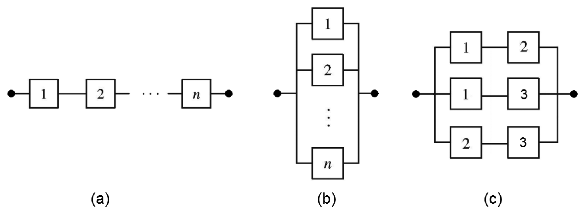
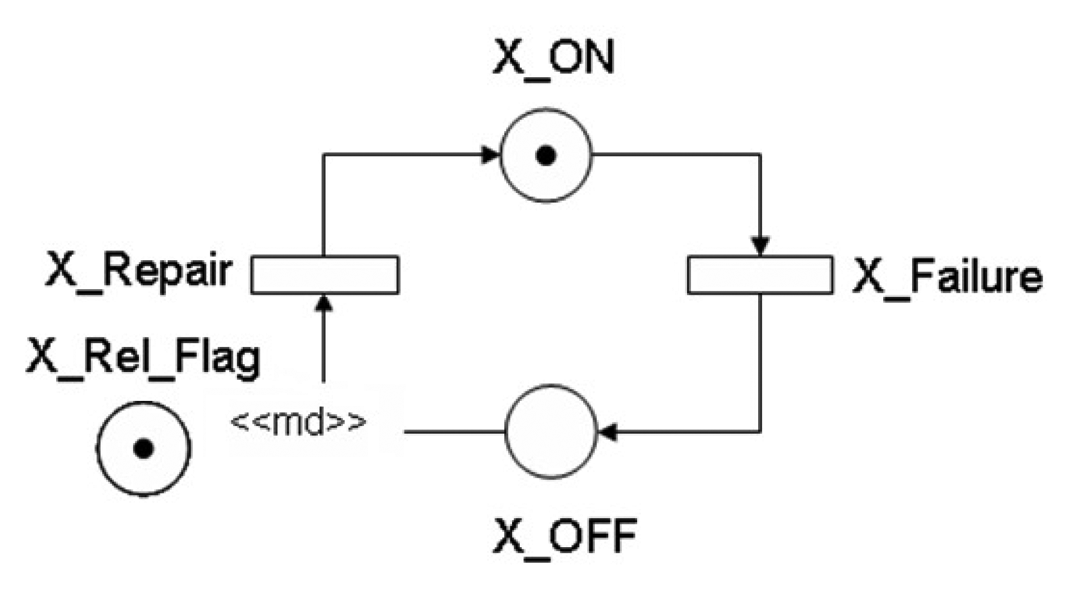
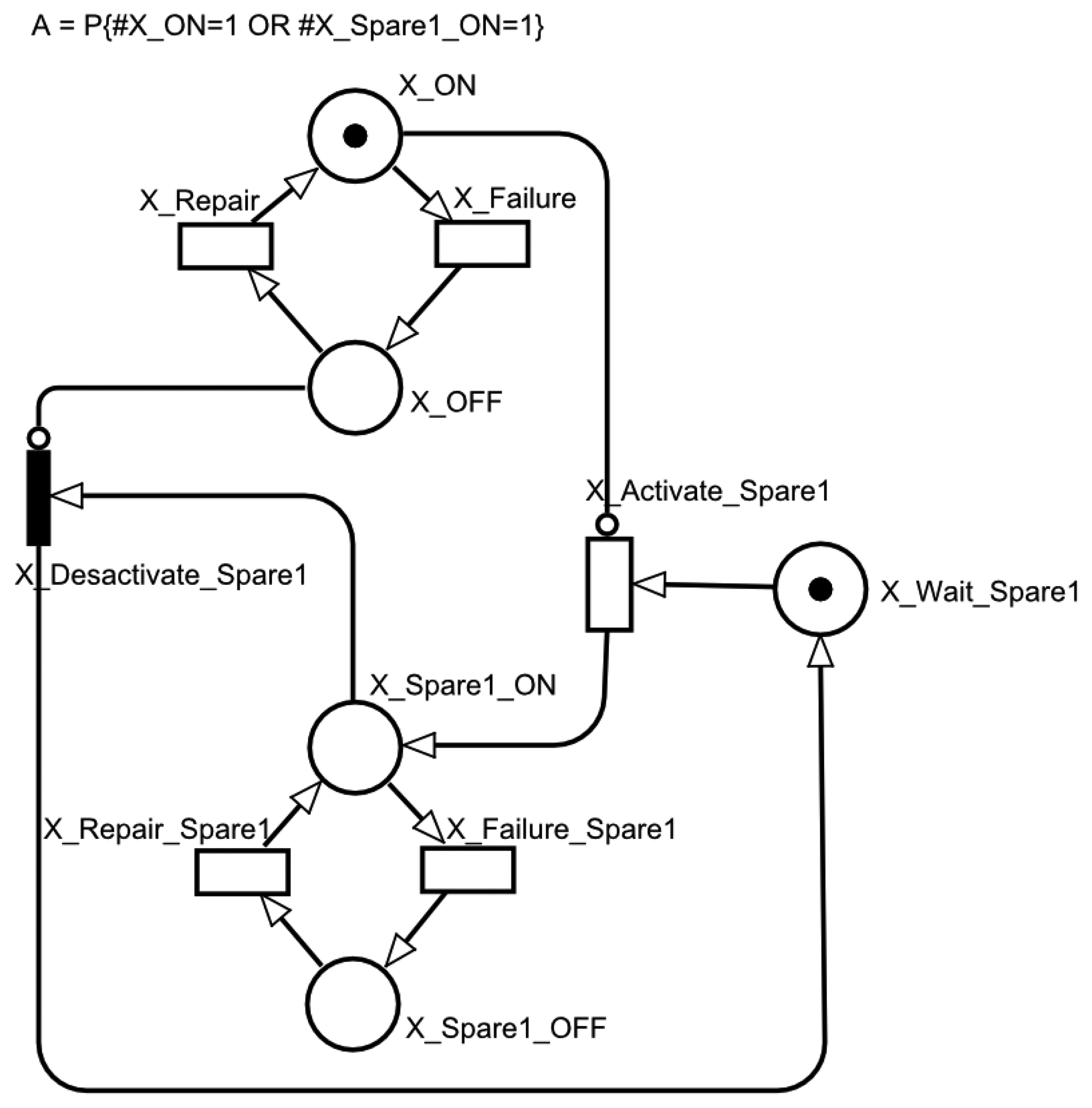
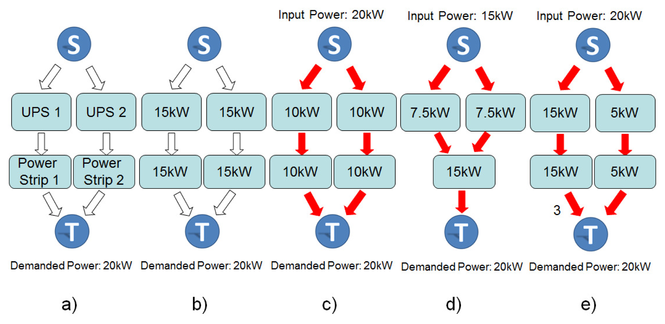
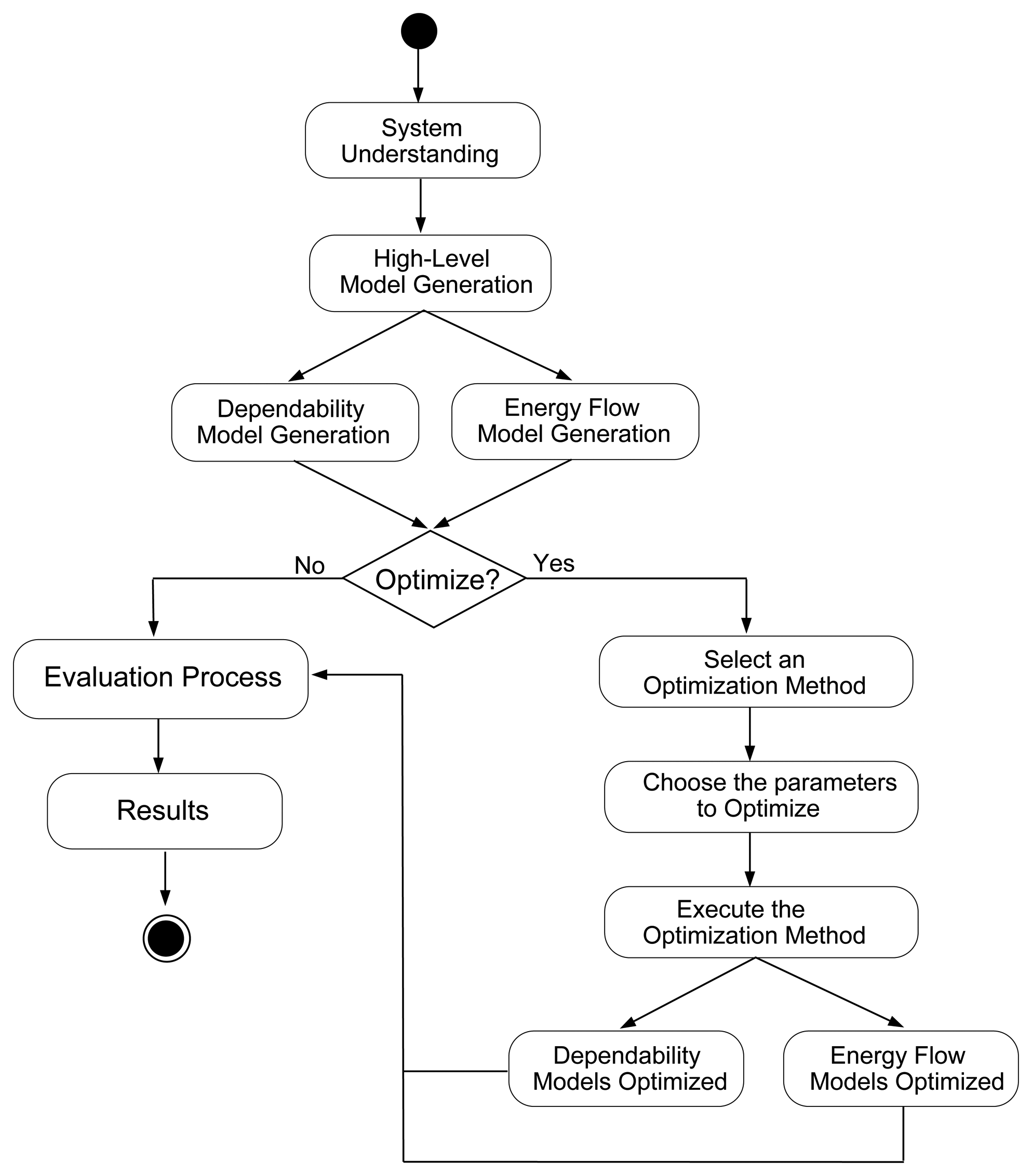
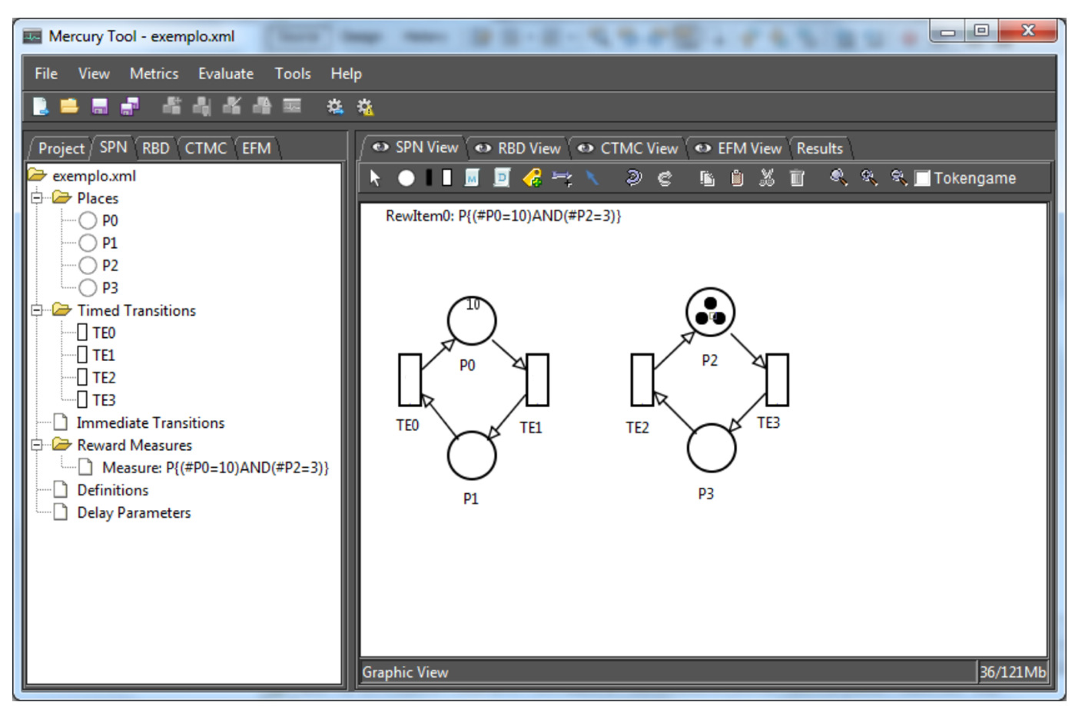
| Transition | Priority | Delay or Weight |
|---|---|---|
| X_Failure | - | X_MTTF |
| X_Repair | - | X_MTTR |
| X_Activate_Spare1 | - | MTActivate |
| X_Failure_Spare1 | - | X_MTTF_Spare1 |
| X_Repair_Spare1 | - | X_MTTR_Spare1 |
| X_Deactivate_Spare1 | 1 | 1 |
| Equipment | MTTF (hs) | AC (USD) | Eff (%) |
|---|---|---|---|
| UPS | [25,000, 75,000] | [11,250, 18,750] | [90.535, 99.9] |
| STS | [24,038, 72,114] | [600, 1,000] | [94.525, 99.9] |
| Subpanel | [152,000, 456,000] | [150, 250] | [94.905, 99.9] |
| Step Down Transformer | [141,290.5, 423,871.5] | [412.50, 687.50] | [93.575, 99.9] |
| Power Strip | [115,111.8, 345,335.3] | [150, 250] | [94.525, 99.9] |
| Arch | Avail (9 s) (Mean) | Down (hs) (Mean) | Down (USD) (Mean) | Acq (USD) (Mean) | Op (USD) (Mean) | Tot (USD) (Mean) | Ex (GJ) (Mean) | Sys Eff (Mean) | ObjFunc (Mean) | Obj Func | Runtime | |
|---|---|---|---|---|---|---|---|---|---|---|---|---|
| A1 | ALL | 0.9998 (3.73) | 1.63 | 326,321.75 | 4,440.85 | 6897.92 | 11,338.77 | 68.09 | 0.7061 | 337,660.52 | 309,658.32 | 2.3 s |
| Opt. | 0.9998 (3.71) | 1.73 | 345,356.08 | 4,587.37 | 6,897.79 | 11,485.17 | 68.09 | 0.7028 | 356,841.25 | 309,658.32 | 2.0 s | |
| Diff | 1.00 (1.01) | 0.94 | 0.94 | 0.97 | 1.00 | 0.99 | 1.00 | 1.00 | 0.95 | 1.00 | 1.20 | |
| A2 | ALL | 0.9998111 (3.72) | 1.66 | 331,007.34 | 8,318.95 | 7,406.41 | 15,725.36 | 84.74 | 0.6551 | 346,732.70 | 323,597.83 | 39.4 s |
| Opt. | 0.9997947 (3.69) | 1.80 | 359,753.32 | 7,783.50 | 7,377.51 | 15,161.01 | 83.79 | 0.6581 | 374,914.34 | 327,659.81 | 4.0 s | |
| Diff | 1.00 (1.01) | 0.92 | 0.92 | 1.07 | 1.00 | 1.04 | 1.01 | 1.00 | 0.92 | 0.99 | 9.64 | |
| A3 | ALL | 0.9998289 (3.77) | 1.50 | 299,701.16 | 8,855.68 | 7,053.88 | 15,909.55 | 73.20 | 0.6875 | 315,610.72 | 284,483.23 | 3 min 27 s |
| Opt. | 0.9998088 (3.72) | 1.67 | 334,940.61 | 8,274.06 | 7,112.76 | 15,386.82 | 75.13 | 0.6815 | 350,327.43 | 293,539.03 | 5.4 s | |
| Diff | 1.00 (1.01) | 0.89 | 0.89 | 1.07 | 0.99 | 1.03 | 0.97 | 1.01 | 0.90 | 0.97 | 38.61 | |
| A4 | ALL | 0.9998462 (3.82) | 1.35 | 269,424.51 | 8,974.10 | 6,584.39 | 15,558.49 | 57.83 | 0.7371 | 284,982.99 | 254,187.48 | 18 min 55 s |
| Opt. | 0.9998382 (3.80) | 1.42 | 283,448.68 | 8,403.39 | 6,572.17 | 14,975.55 | 57.43 | 0.7390 | 298,424.23 | 257,552.05 | 6.6 s | |
| Diff | 1.00 (1.01) | 0.95 | 0.95 | 1.07 | 1.00 | 1.04 | 1.01 | 1.00 | 0.95 | 0.99 | 172.34 | |
| A5 | ALL | 0.99999994 (7.22) | 0.00056 | 112.80 | 7,413.00 | 5,736.13 | 13,149.13 | 30.05 | 0.8425 | 13,261.93 | 12,230.32 | 19 min 39 s |
| Opt. | 0.9999999 (7.20) | 0.00058 | 115.42 | 7,772.58 | 5,796.62 | 13,569.20 | 32.03 | 0.8335 | 13,684.62 | 12,940.75 | 8.1 s | |
| Diff | 1.00 (1.00) | 0.98 | 0.98 | 0.95 | 0.99 | 0.97 | 0.94 | 1.01 | 0.97 | 0.95 | 146.23 | |
| Equipment | MTTF (hs) | AC (USD) | Eff (%) |
|---|---|---|---|
| AC Source | 4,380 | 15,000.00 | 95.3 |
| Generator | 2,500 | 6,000.00 | 25.0 |
| Generator | 3,500 | 7,500.00 | 30.0 |
| Generator | 4,000 | 9,000.00 | 32.0 |
| UPS | 50,000 | 15,000.00 | 95.3 |
| UPS | 60,000 | 16,500.00 | 94.0 |
| UPS | 75,000 | 16,000.00 | 95.3 |
| Step Down Transformer | 282,581 | 550.00 | 98.5 |
| Subpanel | 304,000 | 200.00 | 99.9 |
| Power Strip | 230,223.512 | 200.00 | 99.5 |
| Arch | Avail (9s) | Down (hs) | Down (USD) | Acq (USD) | Op (USD) | Tot (USD) | Exergy (GJ) | Sys Eff | Obj Func | Runtime | |
|---|---|---|---|---|---|---|---|---|---|---|---|
| A6 | ALL | 0.9999418 (4.2349) | 0.5100 | 101,995.61 | 52,900.00 | 10,890.64 | 63,790.64 | 47.1384 | 0.8847 | 165,786.26 | 5 min 03 s |
| Opt. Alg. | 0.9999427 (4.2420) | 0.5017 | 100,352.80 | 54,400.00 | 10,878.26 | 65,278.26 | 44.3915 | 0.8858 | 165,631.06 | 1 min 47 s | |
| Diff | 0.9999991 (0.9983) | 1.0164 | 1.0164 | 0.9724 | 1.0011 | 0.9772 | 1.0619 | 0.9989 | 1.00093 | 2.83 |
| Equipment | MTTF (hs) | AC (USD) | Eff (%) |
|---|---|---|---|
| AC Source | [2,190, 6,570] | [11,250, 18,750] | [90.535, 99.9] |
| Generator | [1,095, 3,285] | [45,000, 75,000] | [23.75, 26.25] |
| Junction box | [2,612,000, 7,836,000] | [112.50, 187.50] | [94.905, 99.9] |
| UPS | [25,000, 75,000] | [11,250, 18,750] | [90.535, 99.9] |
| ATS | [24,038, 72,114] | [600, 1,000] | [94.525, 99.9] |
| Subpanel | [152,000, 456,000] | [150, 250] | [94.905, 99.9] |
| Step Down Transformer | [141,290.5, 423,871.5] | [412.50, 687.50] | [93.575, 99.9] |
| Voltage Panel | [152,000, 456,000] | [150, 250] | [94.905, 99.9] |
| Results | Std. Dev. | [Lower; Upper Bounds] | |
|---|---|---|---|
| Availability (%) | 0.999999781 | 5.519E-08 | [0.999999761; 0.9999998] |
| 9s | 6.67 | 0.107 | [6.63; 6.71] |
| Downtime (hs) | 0.0019 | 0.00048 | [0.0017; 0.0021] |
| Downtime Cost (USD) | 384.17 | 96.69 | [350.14; 418.21] |
| Acquisition Cost (USD) | 211,279.68 | 14349.56 | [206,228.35; 216,331.01] |
| Operational Cost (USD) | 651,540.38 | 46604.69 | [635,134.60; 667,946.16] |
| Total Cost (USD) | 862,820.06 | 49185.47 | [845,505.79; 880,134.32] |
| Exergy Consumption | 6,311.18 | 1621.99 | [5,740.21; 6,882.16] |
| System Efficiency (%) | 0.74 | 0.053 | [0.72; 0.76] |
| Func Objective | 863,204.23 | 49179.92 | [845,891.92; 880,516.54] |
© 2014 by the authors; licensee MDPI, Basel, Switzerland. This article is an open access article distributed under the terms and conditions of the Creative Commons Attribution license( http://creativecommons.org/licenses/by/3.0/).
Share and Cite
Callou, G.; Ferreira, J.; Maciel, P.; Tutsch, D.; Souza, R. An Integrated Modeling Approach to Evaluate and Optimize Data Center Sustainability, Dependability and Cost. Energies 2014, 7, 238-277. https://doi.org/10.3390/en7010238
Callou G, Ferreira J, Maciel P, Tutsch D, Souza R. An Integrated Modeling Approach to Evaluate and Optimize Data Center Sustainability, Dependability and Cost. Energies. 2014; 7(1):238-277. https://doi.org/10.3390/en7010238
Chicago/Turabian StyleCallou, Gustavo, João Ferreira, Paulo Maciel, Dietmar Tutsch, and Rafael Souza. 2014. "An Integrated Modeling Approach to Evaluate and Optimize Data Center Sustainability, Dependability and Cost" Energies 7, no. 1: 238-277. https://doi.org/10.3390/en7010238