A Static Voltage Security Region for Centralized Wind Power Integration—Part I: Concept and Method

Abstract

When large wind farms are centrally integrated in a power grid, cascading tripping faults induced by voltage issues are becoming a great challenge. This paper therefore proposes a concept of static voltage security region to guarantee that the voltage will remain within operation limits under both base conditions and N-1 contingencies. For large wind farms, significant computational effort is required to calculate the exact boundary of the proposed security region. To reduce this computational burden and facilitate the overall analysis, the characteristics of the security region are first analyzed, and its boundary components are shown to be strictly convex. Approximate security regions are then proposed, which are formed by a set of linear cutting planes based on special operating points known as near points and inner points. The security region encompassed by cutting planes is a good approximation to the actual security region. The proposed procedures are demonstrated on a modified nine-bus system with two wind farms. The simulation confirmed that the cutting plane technique can provide a very good approximation to the actual security region.

1. Introduction

In recent years, increasing electricity demands and the need for more environmentally benign electric power systems have become critical concerns to governments and various stakeholders [1,2]. Wind power is one of the most important and readily available renewable resources, and its development has been unprecedentedly rapid.

In China, however, wind resources are mainly distributed in the north and northwest parts of the country, which are far from the major load centers in the eastern and coastal areas. Therefore, wind power is centrally collected and integrated into the power grid and long-distance transmission is necessary to transport the generated wind power to these load centers. The Chinese National Energy Administration (NEA) has set a goal of creating six 10 GW-level wind power bases in wind-rich areas, including Inner Mongolia, Gansu, Xinjiang, Hebei, and Jiangsu, by the end of 2020. These large wind power bases will have to be connected to the power grid via centralized integration.

Due to the intermittent and stochastic characteristics of wind energy, centralized integration of large wind farms introduces new challenges to power system operation. There has been a considerable amount of research on wind power forecasting [3], accommodation [4,5], and economic dispatch [6,7], focusing mainly on active power problems. Probabilistic analysis of small-signal stability was introduced in [8,9] and further enhanced in [10,11], wherein the stochastic density of system-critical eigenvalues (which govern system stability) was determined.

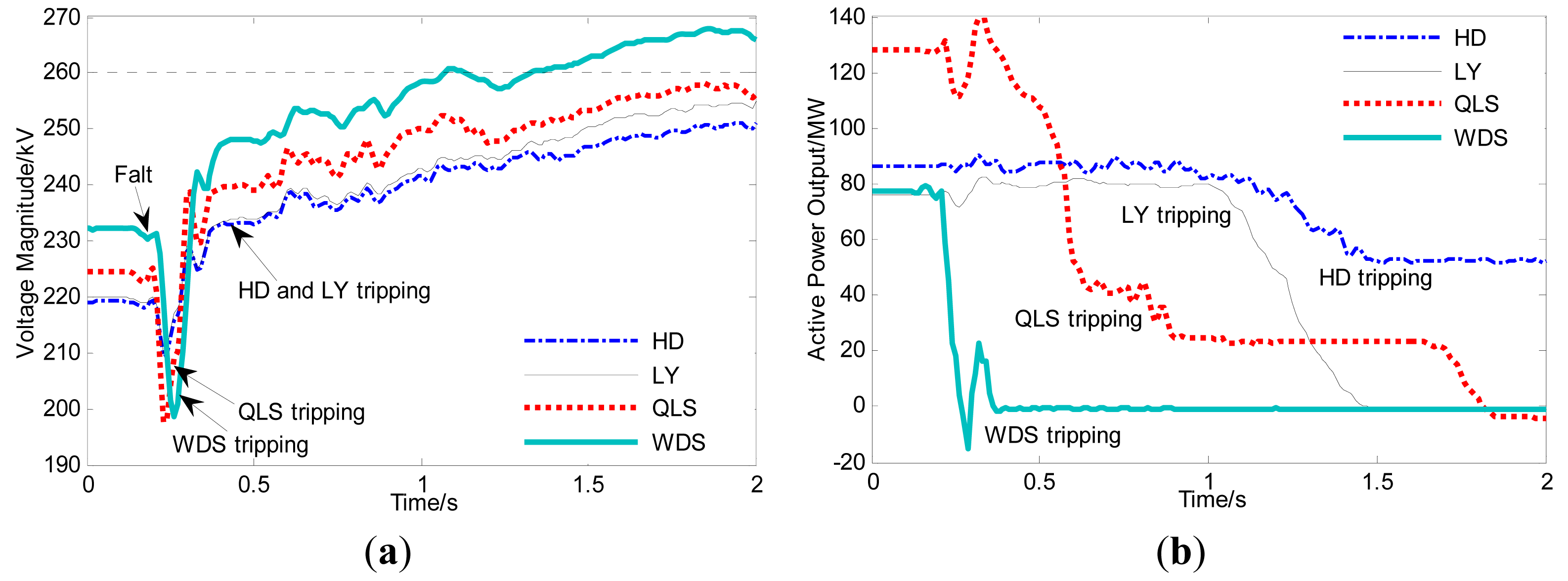
Voltage issues related to wind farm integration have become more significant in recent years. The voltage security of individual wind farms was studied in [12,13] to ensure that bus voltages remained within a specified range, and to improve voltage performance. In [14], a steady-state voltage stability analysis utilizing historical time-series data was proposed for power systems with high penetration of wind power. [15] pointed out that the voltage stability of the regional network might be a main limitation with respect to maximum rating and operation of the wind power plant, and viable measures to enable secure and acceptable operation of large wind farms in remote areas were proposed. Reference [16] presented the voltage stability in a weak connection wind farm and discussed some techniques to improve the transient response of voltage. Furthermore, [17] studied the low voltage ride-through (LVRT) characteristic and the effect that voltage dips had on the operation of the different wind generator topologies. Furthermore, [18] proposed a method to find the steady-state voltage stability region with the consideration of the wind power generation so that it could operate with the voltage within the limits. However, there has been little research on reactive power coordination of wind farms and voltage security in the context of centralized integration of wind farms. Among the centrally integrated wind farms of the northwestern and northern China power grids, several cascading tripping incidents occurred during 2011, causing severe operational problems for the power systems involved. Using synchronized measurements from deployed phasor measurement units (PMUs), these cascading events were recorded. Here, we consider only four wind farms for illustrative purposes. Figure 1 shows the voltage changes in these wind farms, which were connected to the power grid through a 220-kV system.

After a fault occurred at the 35-kV bus of wind farm WDS, the voltage of WDS dropped from 220 kV to 198 kV in 0.22 s, and WDS was tripped first. Afterwards, there were voltage increases at all of the other wind farms. As the voltages continued to rise to about 260 kV, the remaining wind farms started to trip during the time interval from 0.3 s to 2.0 s; most of the wind farms were tripped within 2 s. Some of the wind farms, such as WDS, had all wind units tripped, while others, such as HD, only had some wind units tripped, leading to reduced wind power output. Following the incident, investigators found that such cascading tripping events normally happen during high-wind periods, when wind farm outputs are near the maximum level. The voltages are initially on the lower side, and thus capacitor banks are switched on to provide reactive power compensation. After the fault caused the first wind farm to be tripped, the voltages exceeded the upper operational limit due to lower loading on the transmission lines and slow switch-off of the capacitance banks. The spiked voltages led to further tripping of other wind farms by the overvoltage protection system. This type of cascading tripping event reveals the strong voltage interdependence among centrally integrated wind farms. In the absence of a coordinated voltage control system, voltage security can be at risk. More importantly, in view of the rapid process of a cascading trip incident (barely 2 s, as shown in Figure 1), an effective response is hardly possible once an incident has begun. Hence, preventive control is much more important for maintaining the operational status of closely coupled wind farms, not only under normal operating conditions, but also within acceptable voltage limitations when an N-1 contingency occurs. Therefore, it would be of great value to determine a static voltage security region for typical centralized integrated wind farms, which may be adopted as a set of constraints for automatic voltage control. Note that in this work, an N-1 contingency refers to a single wind farm trip for the sake of convenience.

However, traditional voltage stability region was usually concentrated on the load margin to voltage collapse boundary and prevented the voltage instability by load shedding [19–22]. Whereas centralized wind farms have enough reactive reservation, what we are mainly concerned about is how to adjust the reactive power of each wind farm to mitigate the violation of voltage security constraints. This problem is similar to community activity room (CAR) proposed in [23], but the difference is that CAR is mainly concerned on the transmission capacity constraints by active power adjustment while our work puts emphasis on the correlation of reactive power and voltage.

The remainder of the paper is organized as follows: Section 2 presents the definition of a security region and the associated method for obtaining the exact security region. The characteristics of the security region are then examined, and different techniques are proposed for obtaining a linear approximation of the actual security region, in order to reduce the computational burden. In Section 3, case studies of a nine-bus system with two wind farms are presented. The security region under normal conditions is derived using a sampling-based approach. Approximate security regions are obtained using tangent-plane and cutting-plane methods, and are compared with the actual security region. Our conclusions are stated in Section 4.

2. Static Voltage Security Region and Its Linear Approximation

2.1. Typical Structure of Centralized Wind Farm Integration

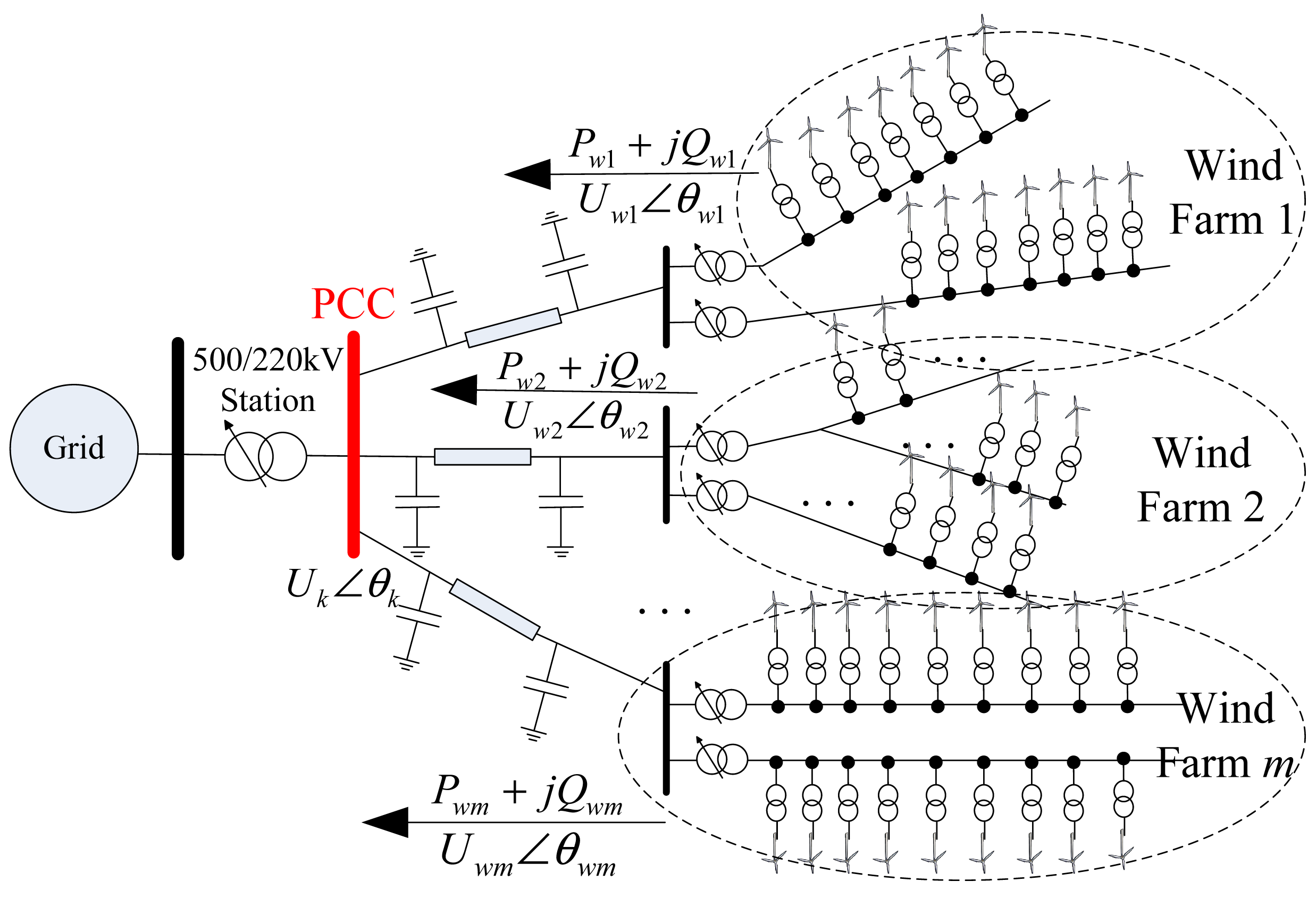
A typical power grid structure for centralized integrated wind farms is shown in Figure 2. First, each wind farm can be regarded as an active distribution network, in which the power injection at each bus is adjustable. Second, each wind farm is usually remote from the load and connected to the grid via long-distance transmission lines, which may result in high charging power. Third, several large-scale wind farms are connected to the same MV busbars of a HV/MV substation (220 kV/500 kV), referred to as the point of common coupling (PCC) in Figure 2. This type of structure is also utilized with other renewable resources (e.g., solar power) to facilitate high penetration, and is very similar to contemplated future distribution grids with high distributed-generator (DG) penetration. Accordingly, this is the typical grid topology considered in the present paper, and may be generalized to applications other than wind farm integration.

2.2. Definition of the Static Voltage Security Region

In choosing the scheduled operating points of wind farms, not only must the network constraints be considered, but also the voltage security of each wind farm. Systems are deployed to protect wind turbine generators against serious over-voltage and low-voltage problems. To avoid triggering these protection systems, the voltage magnitude of each wind farm must be within a certain range centered around a nominal value; i.e., a constraint U ∈ [U_min, U_max] must be satisfied.

Bearing in mind that voltage is an algebraic state variable and reactive power is a control variable, to guarantee that the voltage remains within the safety region, the reactive power must be restricted. Therefore, the static voltage security region of wind farms can be expressed as a set of constraints limiting the reactive power of each wind farm to maintain its static nodal voltage in the secure range, given the active power generation of each wind farm. Of course, the static voltage security region of wind farms will vary with the level of active power generation. In addition, the reactive capacity limit of each wind farm must be examined in detail, based on the following considerations:

(i)

The designed power factor, which for a DIFG wind turbine, normally ranges from capacitive 0.95 to inductive 0.95. For example, the reactive power should vary from −500 kVar to +500 kVar for one 1.5-MW DFIG wind turbine. For a wind farm with several wind turbines, the total reactive power output range is the combined reactive power output range for all wind turbines on the farm;

(ii)

Operating requirements (quality, economy, and security);

(iii)

Reactive power compensation for each wind farm.

The reactive power constraints for the wind farms can be expressed as:

$$\underset{\_}{Q_i}\le Q_i\le \overline{Q_i},i\in \mathit{w}$$

(1)

Let x = [U,θ], y = [P_g, Q_g, P_l, Q_l, P_w], and z = Q_w. According to the definition of the static voltage security region, the following requirements must be satisfied for any secure operating point:

$$f(\mathit{x},\mathit{y},\mathit{z})=0$$

(2)

$$g(\mathit{x},\mathit{y},\mathit{z})\le 0$$

(3)

$$\begin{array}{l}\underset{\_}{{\mathit{x}}_w}\le {\mathit{x}}_w\le \overline{{\mathit{x}}_w}\\ \underset{\_}{\mathit{z}}\le \mathit{z}\le \overline{\mathit{z}}\end{array}$$

(4)

Equation (2) represents the active and reactive energy balance equations. Equations (3) and (4) represent the transmission capacity limit, the reactive power limits of the wind farms, and the safe voltage range, respectively. We let Ω_S denote the initial static voltage security region, which does not incorporate the reactive power limits, and Ω_VSR denote the final static voltage security region. The two regions can be written as follows:

$${\Omega }_{\text{S}}=\{\mathit{z}\in R^m|\mathit{f}(\mathit{x},\mathit{y},\mathit{z})=0,\mathit{g}(\mathit{x},\mathit{y},\mathit{z})\le 0,X^D\}$$

$${\Omega }_{\text{VSR}}={\Omega }_{\text{S}}\cap \underset{\_}{{\mathit{z}}_w}\le {\mathit{z}}_w\le \overline{{\mathit{z}}_w}$$

where $X^D:\underset{\_}{{\mathit{x}}_w}\le {\mathit{x}}_w\le \overline{{\mathit{x}}_w}$.

In fact, Ω_VSR is the static voltage security region under normal condition (also called N-0). Based on it, we can further define the N-1 security region and N-k security region, to guarantee the security under N-1 contingency and even N-k contingency.

Suppose wind farm i is tripped. Then the active power drops to zero, while the reactive power only excludes the generation from the wind units and the others should remain unchanged to simulate the slow switch-off of the capacitance banks and shunt capacitance of long-distance transmission lines (i.e., the capacitance banks and shunt capacitance of long-distance transmission lines remain unchanged) Hence, the dimension of the N-1 static voltage security region is still m, and the desired region is given by:

$${\Omega }_{\text{VSR}}^{N-1}=\underset{i=0}{\overset{m}{\cap }}({\Omega }_{\text{VSR}}^i|P_w^i=0)$$

(5)

where ${\Omega }_{\text{VSR}}^i$ denotes the security region when wind farm i is tripped (i = 1, …, m). The N-1 security region is actually bounded by 2m(m+1) planes before reactive limits are imposed. It is simply the intersection of m+1 security region planes, and is also a convex set.

Similarly, if any k wind farms are tripped, that is ∀{N₁, …, N_k} ⊆ {1, …, m}, then the N-k security region can be formed as Equation (6). Obviously, this region is an intersection of $C_m^k$ security regions:

$${\Omega }_{\text{VSR}}^{N-k}=\underset{i=0}{\overset{C_m^k}{\cap }}{\Omega }_{\text{VSR}}^i|\{P_w^{N_1}=0,\mathrm{\dots },P_w^{N_k}=0\}$$

(6)

However, in this work, for convenience and in order to mitigate the cascading trips, the region should ensure secure operation both under normal operating conditions and N-1 contingencies. If an operating point is in the normal security region, but out of the N-1 region, this means that cascading is probably triggered by the first trip. Thus, even if the current operating status is normal, it is not secure enough, and preventive control measures should be carried out according to the proposed N-1 voltage security region.

It is of course obvious that normal voltage security region is the basis for N-1 voltage security region. Therefore, we will put emphasis on the calculation of normal voltage security region in the following work, and the N-1 security region will be fully studied in part II [24].

2.3. Characteristics of the Static Voltage Security Region

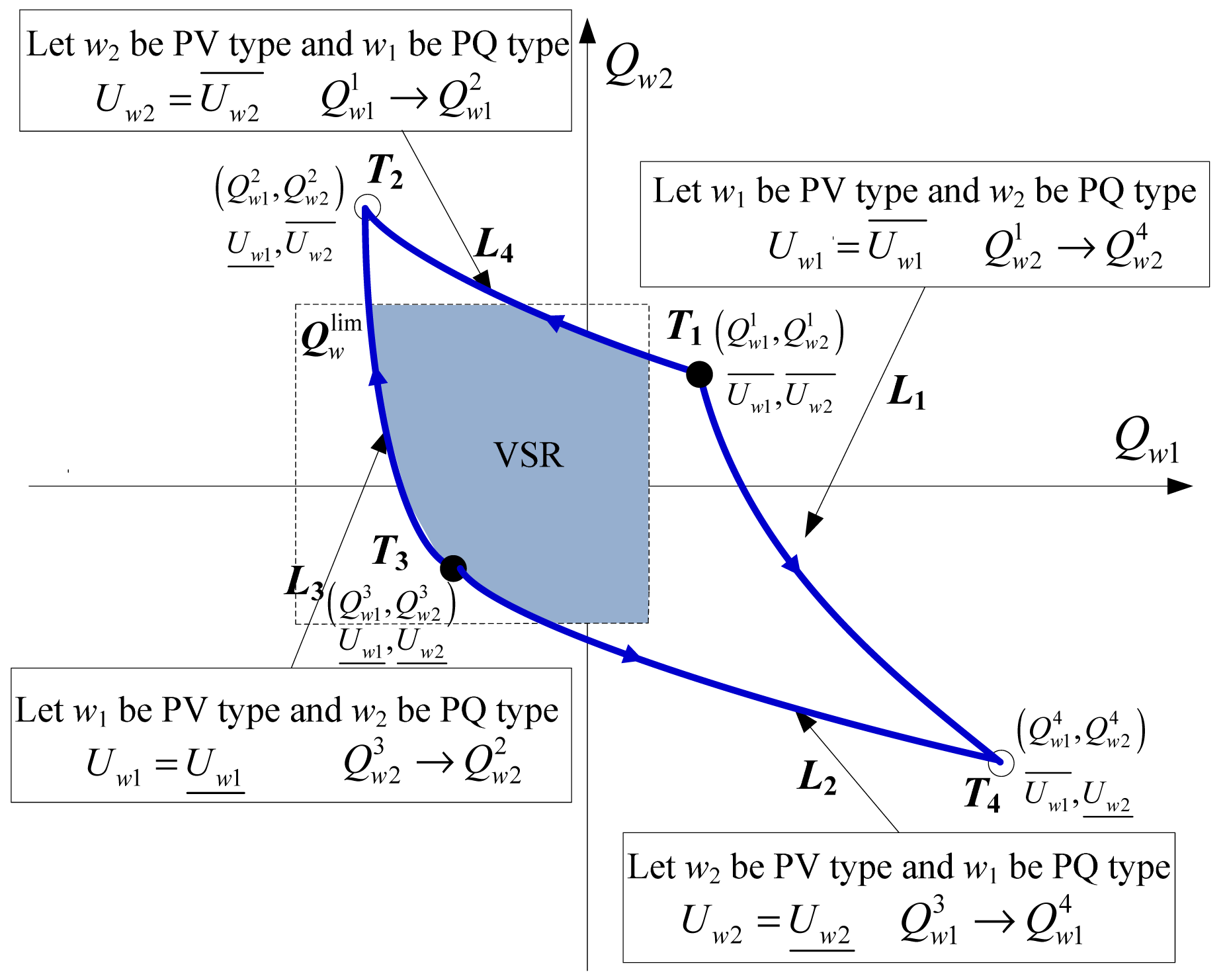
A sampling-based approach can be employed to identify the static voltage security region. For a single wind farm, the security region can easily be expressed as an interval. For two or more wind farms, a sampling-based approach can be effective for determining the security region. For the sake of simplicity, the process is illustrated for two wind farms, which involves two independent variables. The procedure can be found in Appendix I. The security region constructed by this method (shown in Figure 3) can be expressed as follows:

$${\Omega }_{\text{S}}=\{(Q_{w1},Q_{w2})|(Q_{w1},Q_{w2})\in S(L_1,L_2,L_3,L_4)\},{\Omega }_{\text{VSR}}={\Omega }_{\text{S}}\cap {\mathit{Q}}_w^{lim}.$$

where S denotes the area enclosed by the curves L₁, L₂, L₃, and L₄, and ${\mathit{Q}}_w^{lim}$ denotes the area obtained from the reactive power constraints of (1).

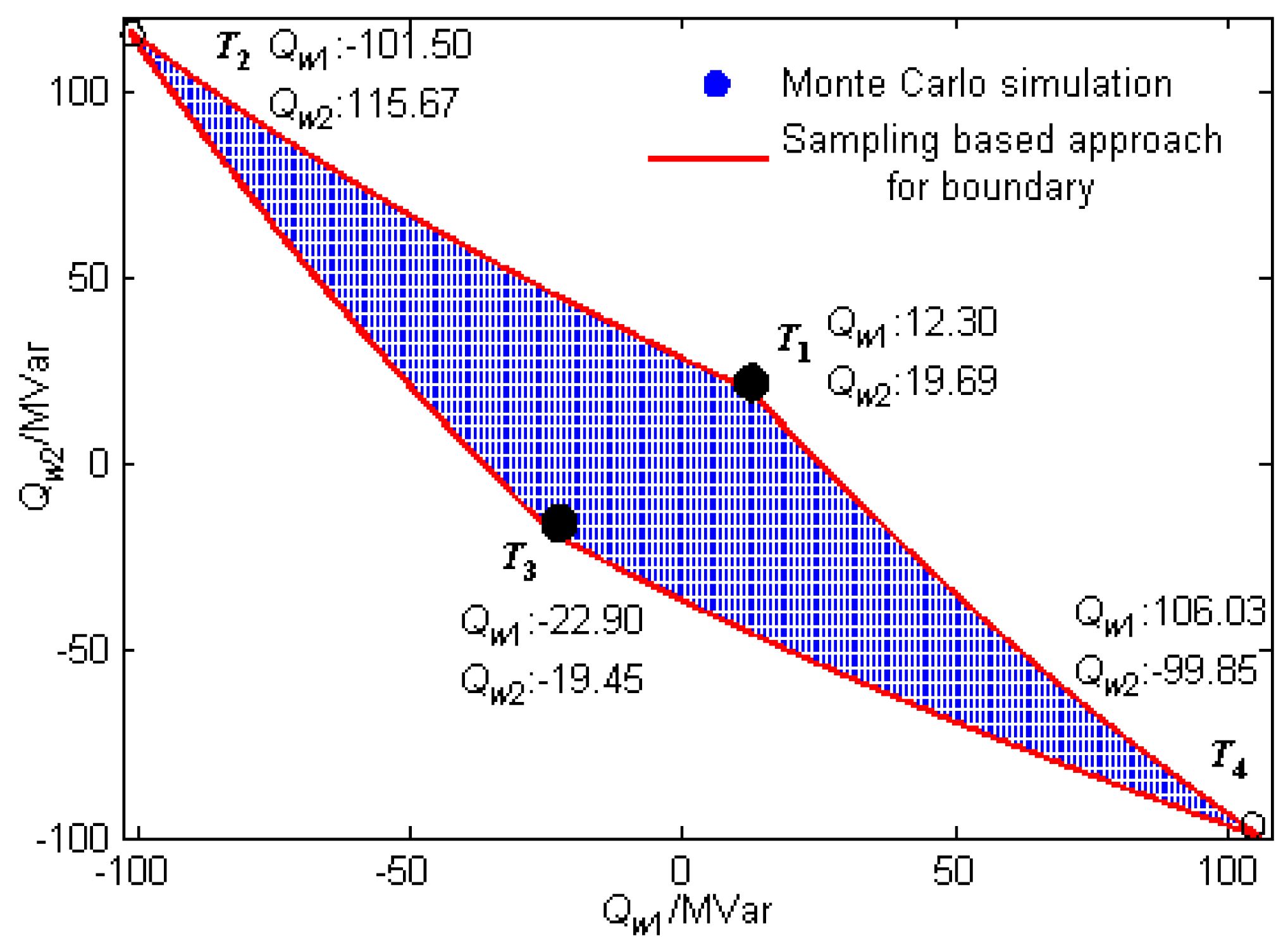
In Figure 3, both wind farms reach the upper bounds of their respective voltage magnitudes at point T₁, and lower bounds at point T₃. At points T₂ and T₄, one wind farm reaches the upper bound while the other reaches the lower bound. In this paper, T₁ and T₃ are termed near points, since they are near the center of the security region, whereas T₂ and T₄ are called remote points, since they are relatively distant from the center of the security region.

A number of characteristics of the security region from the sampling-based approach have been observed, and are summarized as follows:

• (C-1) The boundary of the security region approximate to a linear form but not strictly equivalent to it, and the security region is bounded by a closed set.

• (C-2) All elements of the Q–U sensitivity matrix are positive, and the diagonal elements are greater than the off-diagonal elements.

• (C-3) Each remote point is either above and to the left or below and to the right of a near point, which means the slope of each boundary curve is negative.

Actually, the wind farms are usually taken as PQ buses, so the boundaries of security region are actually the case where the voltage magnitude of some PQ buses exceed their limits, so that these PQ bus should be converted to PV bus. Note that, it is different from the limit induced bifurcation (LIB) which is related to the PV bus whose reactive power exceeds its limits, so that the PV bus should be converted to PQ bus [25].

2.4. Security Region Boundary and Linear Approximation

For large-scale integration of m wind farms, m-dimensional variables appear in the reactive power constraints. Although the number of near points is still two, the number of remote points becomes 2^m − 2. When m is a large number, it is computationally expensive to calculate the security region Ω_S and its boundary using the sampling-based approach. Monte Carlo simulation is perhaps a feasible method for achieving the same goal, but no mathematical expression can be derived to facilitate an in-depth analytical study. Therefore, it is of great interest to approximate Ω_S by regions having convenient mathematical representations.

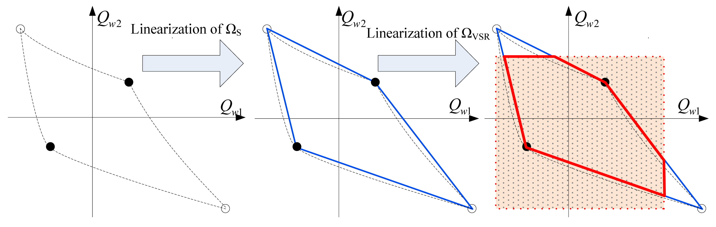
The final security region Ω_VSR is simply the intersection of the initial security region Ω_S and the reactive power limits Q^lim; only the initial security region Ω_S involves nonlinearity. Therefore, we will concentrate on approximating Ω_S. Since the security region is a space enclosed by nonlinear boundary curves, a good approximation to the boundary will naturally produce a good approximation to the security region itself.

The voltage drop due to the reactance between the PCC and the wind farms causes nonlinearity in the security region boundary curves, and thus makes it difficult to represent these curves mathematically. However, it is possible to approximate the nonlinear boundary curves with linear counterparts across the near points when the voltage drop is small. Figure 4 illustrates the process of obtaining a linear approximation for the security region Ω_S in a two-dimensional case. The dashed lines represent the boundary of the actual security region Ω_S, and the solid lines represent linear approximations of the boundary curves. The shaded area represents the reactive power limits ${\mathit{Q}}_w^{lim}$. The details of the linear approximation procedures will be discussed in the next subsection.

By the Newton–Raphson method, we obtain the following system of linear equations:

$$\left[\begin{array}{l}\mathrm{\Delta }\mathit{P}\\ \mathrm{\Delta }\mathit{Q}\end{array}\right]=-\left[\begin{array}{cc}{\mathit{J}}_{\text{P}\theta }& {\mathit{J}}_{\text{PU}}\\ {\mathit{J}}_{\text{Q}\theta }& {\mathit{J}}_{\text{QU}}\end{array}\right]\left[\begin{array}{l}\mathrm{\Delta }\theta \\ \mathrm{\Delta }\mathit{U}\end{array}\right]$$

(7)

If the effect of real power changes is neglected (i.e., ΔP = 0), this leads to:

$$\mathrm{\Delta }Q=[{\mathit{J}}_{\text{QU}}-{\mathit{J}}_{\text{Q}\theta }{\mathit{J}}_{\text{P}\theta }^{-1}{\mathit{J}}_{\text{PU}}]\mathrm{\Delta }U$$

(8)

$$\mathrm{\Delta }Q={[{\mathit{J}}_{\text{QU}}-{\mathit{J}}_{\text{Q}\theta }{\mathit{J}}_{\text{P}\theta }^{-1}{\mathit{J}}_{\text{PU}}]}^{-1}\mathrm{\Delta }U$$

(9)

If H = [J_QU − J_QθJ_Pθ^–1J_PU]^–1, the following equation represents the net active and reactive power flow for the wind farms only:

$$\mathrm{\Delta }{\mathit{U}}_w={\mathit{H}}_{\mathit{\text{ww}}}\mathrm{\Delta }{\mathit{Q}}_{w}w\in \mathit{w}$$

(10)

However, the sensitivity matrix approximates to $\frac{\mathrm{\Delta }U}{\mathrm{\Delta }Q}\approx {(\mathit{B}”)}^{-1}$ with respect to the P-Q decompled power flow, which reflects the electrical distance. Hence, the diagonal elements are greater than the off-diagonal elements.

Take the boundary curve L₁ for example. When T₁ moves to T₄, the voltage magnitude of wind farm w₂ drops from $\overline{U_{w2}}$ to $\underset{\_}{U_{w2}}$, whereas U_w1 remains constant (i.e., ΔU_w1 = 0). In other words, the first line of matrix H_ww in Equation (10) is zero, and we can conclude that if Q_w2 decreases, Q_w1 increases (i.e., ∂Q₂/∂Q₁ > 0), since the elements of H_ww are positive according to (C-2). Intuitively speaking, the relationship between ΔQ_w1 and ΔQ_w2 should be linear in accordance with (10), but the loss change is nonlinear with the system power change, and hence the boundary of Ω_VSR is more or less convex.

In order to measure how well the nonlinear boundary components of the security region can be approximated by linear counterparts, the following linearity index is defined to represent the degree of linearity of the components:

$$L_a=\frac{\sqrt{\frac{1}{m}\text{∑}_{i=1}^m{({U_i|}_{\text{near point}}-U_{\text{PCC}})}^2}}{\sqrt{\frac{1}{m}\text{∑}_{i=1}^m{U_i^{\text{2}}|}_{\text{near point}}}}\times 100\%$$

(11)

where m is the total number of wind farms, and U_i|nearpoint and U_PCC are the respective voltages of wind farm i and the PCC bus at the near point. The smaller the value of the index, the closer a nonlinear boundary component is to its linear counterpart.

2.5. Linear Approximation Procedures

On the boundary of the security region, the voltage magnitudes at some wind buses tend to reach their upper bounds $\overline{U_w}$ or lower bounds $\underset{\_}{U_w}$; these buses will be changed to the PV type.

Suppose ξ = (ε₁, ε₂, …, ε_m)^T ∈ ℜ^m, where ε_i =0 or ±1, i = 1, …, m. The value 0 indicates PQ type; +1 indicates PV type with a voltage magnitude equal to the upper bound and −1 indicates PV type with a voltage magnitude equal to the lower bound. The set containing the two near points ξ⁻ = (−1, −1, …, −1)^T and ξ⁺ = (−1, −1, …, −1)^T is denoted by N_p, while the set of 2^m – 2 remote points (±1, ±1, …, ±1)^T/N_p is denoted by R_p.

The boundary of Ω_S is comprised of nonlinear hypersurfaces in multi-dimensional space. If we want to approximate the boundary with hyperplanes, we are confronted with problems such as how many hyperplanes are needed and how to select them. At the very least, the 2^m – 2 remote points must be dealt with, and this involves formidable computations. It is of great interest to develop a technique for approximating the voltage security region using only the two near points and none of the numerous remote points.

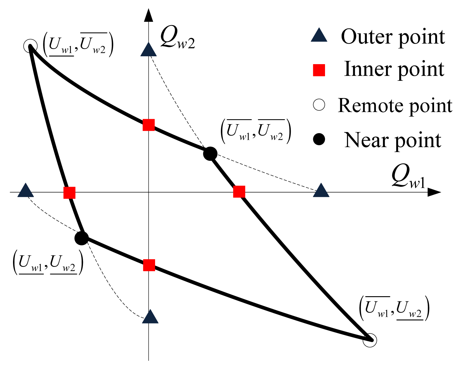
In order to develop a linear approximation method using only the near points, we first define two additional concepts: the inner point and outer point. These two types of special operating points are illustrated in Figure 5, together with near points and remote points. Let η = (η₁, η₂, …, η_m)^T ∈ ℜ^m be a point. Then, the inner point η̆ is the point such that one component η_i equals 0 when it varies from $\underset{\_}{{\eta }_i}$ to $\overline{{\eta }_i}$; that is:

$$\{\eta ={({\eta }_1,\mathrm{\dots },{\eta }_m)}^T|{\mathit{\varepsilon }}_i=0,{\mathit{\varepsilon }}_{\forall k,k\ne i}\ne 0,{\eta }_i=0,{\eta }_{\forall k,k\ne i}\ne 0\}$$

(12)

The outer point is the point such that any other component except η_i equals 0 when the component η_i varies from $\underset{\_}{{\eta }_i}$ to $\overline{{\eta }_i}$; that is:

$$\{\mathbf{\eta }={({\eta }_1,\mathrm{\dots },{\eta }_m)}^T|{\mathit{\varepsilon }}_i=0,{\mathit{\varepsilon }}_{\forall k,k\ne i}\ne 0,{\eta }_i\ne 0,{\eta }_{\forall k,k\ne i}=0\}$$

(13)

Inner points and outer points are special operating points. An inner point represents an operating point where one wind generator bus is a PQ bus with 0 Mvar injection, and all other wind generator buses are PV buses. An outer point represents an operating point where one wind generator bus is a PQ bus and all other wind generator buses are PV buses, one of which has 0 Mvar injection. Therefore, an inner point can be determined by a single power flow calculation, while an outer point requires a sampling approach. Thus, inner points are easier to calculate than outer points.

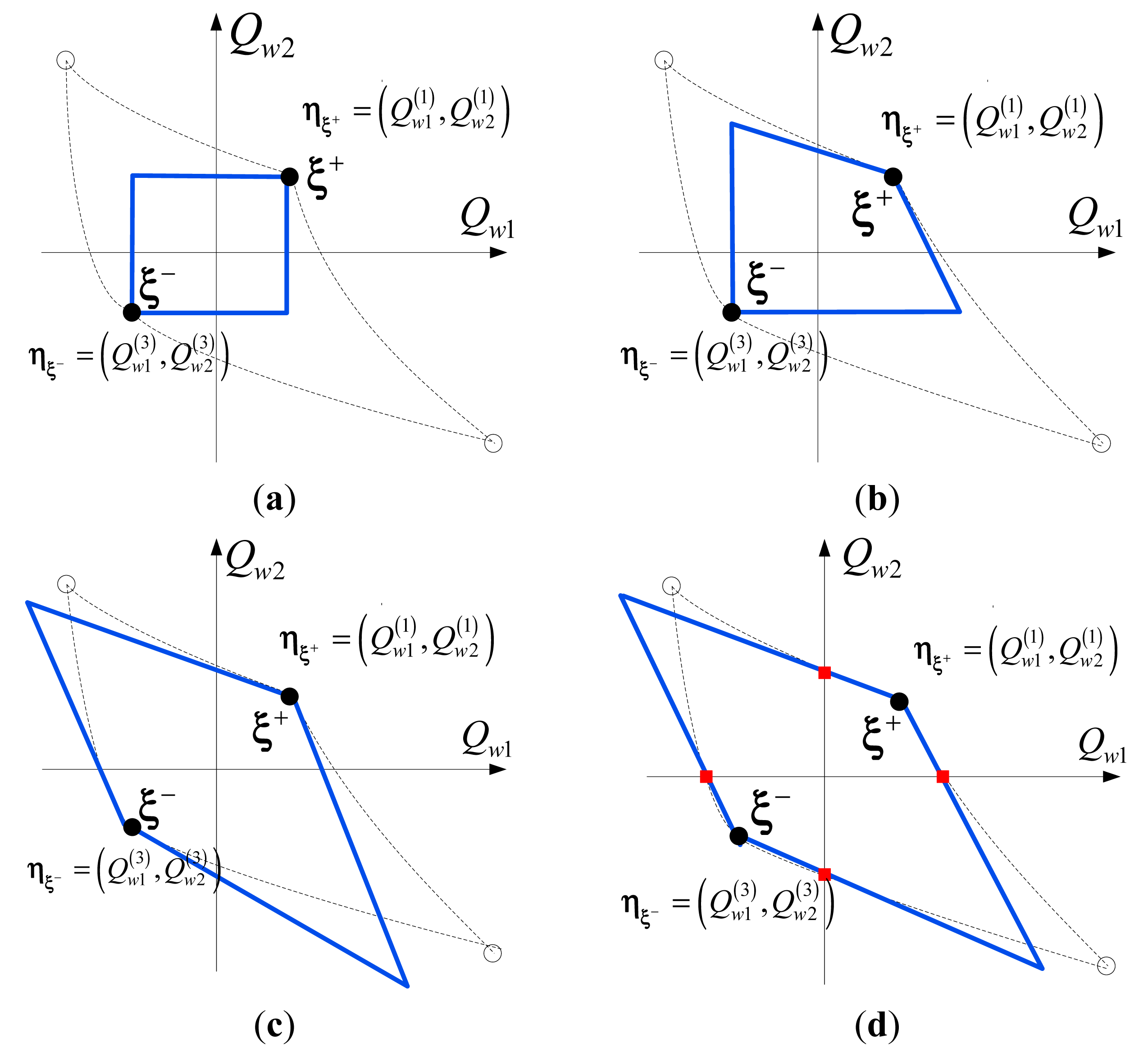
At different levels of computational difficulty, four distinct techniques are proposed to approximate the boundary components of Ω_S, using near points and/or inner points. The approximate boundary is the union of 2m hyper-planes in m-dimensional space. Figure 6 illustrates the four techniques in a two-dimensional case. Figure 6a depicts a technique using only near points. It requires the fewest computations, but the resulting security region is the most conservative. By devoting additional computations to calculating the tangent hyperplanes at one of the near points ξ⁺, the technique illustrated in Figure 6b achieves a security region that covers more of the actual region. However, the portion of the actual security region near the remote points is still neglected. Figure 6c utilizes tangent hyperplanes at both near points, so that the approximate security region covers much more of the actual region. However, due to the convexity of the boundary components, the tangent hyper-planes near point ξ⁻ will create an “overspill” effect, where part of the approximate security region is outside the actual security region. Figure 6d uses near points and inner points to construct cutting planes, and the resulting approximate security region spans most of the actual region, with limited “overspill”. The technique of Figure 6d is the one recommended in this paper. It should also be noted that the higher the linearity of the actual security region, the better the approximations of Figure 6c,d become. The four different linear approximations of the security region can be expressed as follows:

• $(6\text{a}):{\Omega }_{\text{S}}^0=\{{(Q_{w1},\dots ,Q_{wm})}^T|Q_{wi}^{(3)}\le Q_{wi}\le Q_{wi}^{(1)},i=1,\dots ,m\};$

• $(6\text{b}):{\Omega }_{\text{S}}^0=\{{(Q_{w1},\dots ,Q_{wm})}^T|Q_{wi}^{(3)}\le Q_{wi}\cap \nabla ({\mathbf{\eta }}_{{\xi }^{+}})\le 0,i=1,\dots ,m\};$

• $(6\text{c}):{\Omega }_{\text{S}}^0=\{{(Q_{w1},\dots ,Q_{wm})}^T|\nabla ({\mathbf{\eta }}_{{\xi }^{-}})\ge 0\cap \nabla ({\mathbf{\eta }}_{{\xi }^{+}})\le 0\};$

• $(6\text{d}):{\Omega }_{\text{S}}^0=\{{(Q_{w1},\dots ,Q_{wm})}^T|\mathrm{\Delta }({\mathbf{\eta }}_{{\xi }^{-}},\stackrel{⌣}{\mathbf{\eta }})\ge 0\cap \mathrm{\Delta }({\eta }_{{\xi }^{+}}\stackrel{⌣}{\eta })\le 0\}.$

where “0” denotes the normal working point, ∇ denotes the tangent plane at the near point, which can easily be obtained from the Q − U matrix H_ww at the near point using Equation (10), and Δ denotes the cutting plane through the near point and the inner points.

The details of the technique shown in Figure 6d are as follows. There are m planes across the near points ξ⁺ and ξ⁻, respectively denoted by Θ_ξ− = {L₁⁺, …, L_i⁺, …, L_m⁺} and Θ_ξ− = {L₁⁻, …, L_i⁻, …, L_m⁻}. L_i⁺ and L_i⁻ represent the i^th planes across the near points ξ⁺ and ξ⁻, respectively. Let plane L_i⁺ and plane L_i⁻ be represented by $\text{∑}_{k=1}^m{\alpha }_{i,k}^{+}{Q}_k=1$ and $\text{∑}_{k=1}^m{\alpha }_{i,k}^{-}{Q}_k=-1$, respectively, where α_i,k⁺ and α_i,k⁻ represent the coefficients of planes L_i⁺ and L_i⁻. Let the m inner points associated with the near point ξ⁺ be denoted by ${\stackrel{⌣}{\mathbf{\eta }}}_1^{+},\mathrm{\dots }{\stackrel{⌣}{\mathbf{\eta }}}_i^{+}\mathrm{\dots },{\stackrel{⌣}{\mathbf{\eta }}}_m^{+}$. Each plane is uniquely determined by m – 1 inner points and one near point. For instance, utilizing the near point and all the inner points except ${\stackrel{⌣}{\mathbf{\eta }}}_i^{+}$, we have $({\stackrel{⌣}{\mathbf{\eta }}}_1^{+},\mathrm{\dots },{\stackrel{⌣}{\mathbf{\eta }}}_{i-1}^{+},{\mathbf{\eta }}_{{\xi }^{+}},{\stackrel{⌣}{\mathbf{\eta }}}_{i+1}^{+},\mathrm{\dots },{\stackrel{⌣}{\mathbf{\eta }}}_m^{+})$, where:

$$({\stackrel{⌣}{\mathbf{\eta }}}_1^{+},\mathrm{\dots },{\stackrel{⌣}{\mathbf{\eta }}}_{i-1}^{+},{\mathbf{\eta }}_{{\xi }^{+}},{\stackrel{⌣}{\mathbf{\eta }}}_{i+1}^{+},\mathrm{\dots },{\stackrel{⌣}{\mathbf{\eta }}}_m^{+})={\left(\begin{array}{ccc}{Q}_{11}& \dots & Q_{1m}\\ ⋮& \ddots & ⋮\\ Q_{m1}& \cdots & Q_{mm}\end{array}\right)}^T$$

(15)

These points can be used to uniquely determine the coefficients ${\mathbf{\alpha }}_i^{+}={({\alpha }_{i,1}^{+},\mathrm{\dots },{\alpha }_{i,m}^{+})}^T$ of plane $L_i^{+}$. Since the total number of inner points associated with each near point is m, a total of C_m^{m – 1} = m planes will be determined by a near point and the m inner points. Thus, Θ_ξ+ can be determined using the near point ξ⁺ and the inner pointsbe. Similarly, Θ_ξ− can be determined using the near point ξ⁻ and the inner points ${\stackrel{⌣}{\mathbf{\eta }}}_1^{-},\mathrm{\dots },{\stackrel{⌣}{\mathbf{\eta }}}_m^{-}$, with the coefficients ${\alpha }_i^{-}={({\alpha }_{i,1}^{-},\mathrm{\dots },{\alpha }_{i,m}^{-})}^T$ of each plane $L_i^{-}$. Then, Θ_ξ+ and Θ_ξ− can be represented as:

$${\Theta }_{{\xi }^{+}}\triangleq {\mathit{A}}^{+}\left[\begin{array}{c}{Q}_1\\ ⋮\\ Q_m\end{array}\right]=\left[\begin{array}{c}1\\ ⋮\\ 1\end{array}\right],{\Theta }_{{\xi }^{-}}\triangleq {\mathit{A}}^{-}\left[\begin{array}{c}{Q}_1\\ ⋮\\ Q_m\end{array}\right]=\left[\begin{array}{c}-1\\ ⋮\\ -1\end{array}\right]$$

(16)

where:

$${\mathit{A}}^{+}={({\mathit{\alpha }}_1^{+},\mathrm{\dots },{\mathit{\alpha }}_m^{+})}^T=\left(\begin{array}{ccc}{\alpha }_{11}^{+}& \dots & {\alpha }_{1m}^{+}\\ ⋮& \ddots & ⋮\\ {\alpha }_{m1}^{+}& \cdots & {\alpha }_{mm}^{+}\end{array}\right),{\mathit{A}}^{-}={({\mathit{\alpha }}_1^{-},\mathrm{\dots },{\mathit{\alpha }}_m^{-})}^T=\left(\begin{array}{ccc}{\alpha }_{11}^{-}& \dots & {\alpha }_{1m}^{-}\\ ⋮& \ddots & ⋮\\ {\alpha }_{m1}^{-}& \cdots & {\alpha }_{mm}^{-}\end{array}\right)$$

(17)

Therefore, the voltage security region ${\Omega }_{\text{S}}^0$ is the area enclosed by Θ_ξ+ and Θ_ξ+. Considering the reactive limits, the security region can be finally expressed as: ${\Omega }_{\text{VSR}}^0={\Omega }_{\text{S}}^0\cap {\mathit{Q}}^{lim}$

3. Simulation

The nine-bus test system of [26] was chosen for the numeric studies. The system was modified by adding two new buses for connecting additional wind farms. Thus, there were eleven buses altogether. The two new buses, as well as Bus 2, were connected to Bus 8, which was utilized as the PCC of the wind farms. The parameters and the topology can be observed in Appendix II.

We assumed that the feasible voltage range of each wind farm was [0.9 p.u., 1.1 p.u.]; i.e., $\overline{U_w}=1.1$ and $\underset{\_}{U_w}=0.9$. The power flow was determined using the MATPOWER toolbox [26]. The voltage security region under normal conditions was illustrated for a case in which two wind farms were connected to the PCC.

3.1. Initial Voltage Security Region (Ω_S)

In this section, two wind farms were connected to the PCC at Bus 8. The active powers of the two wind farms were P_w1 = 80 MW and P_w2 = 160 MW, respectively. After the power flow was determined, the two near points and two remote points were obtained. As in Figure 3, near point T₁ was η_ξ⁺ = (12.30, 19.69) Mvar and near point T₃ was η_ξ⁻ = (−22.90, −19.45) Mvar. The two remote points T₂ and T₄ were (−101.50, 115.87) Mvar and (106.03, −99.85) Mvar, respectively. The computed boundary curves could be verified by Monte Carlo simulation. Figure 7 shows the boundary curves obtained via the sampling-based approach and those obtained via Monte Carlo simulation. The boundary curves coincided precisely with those of the actual security region Ω_S.

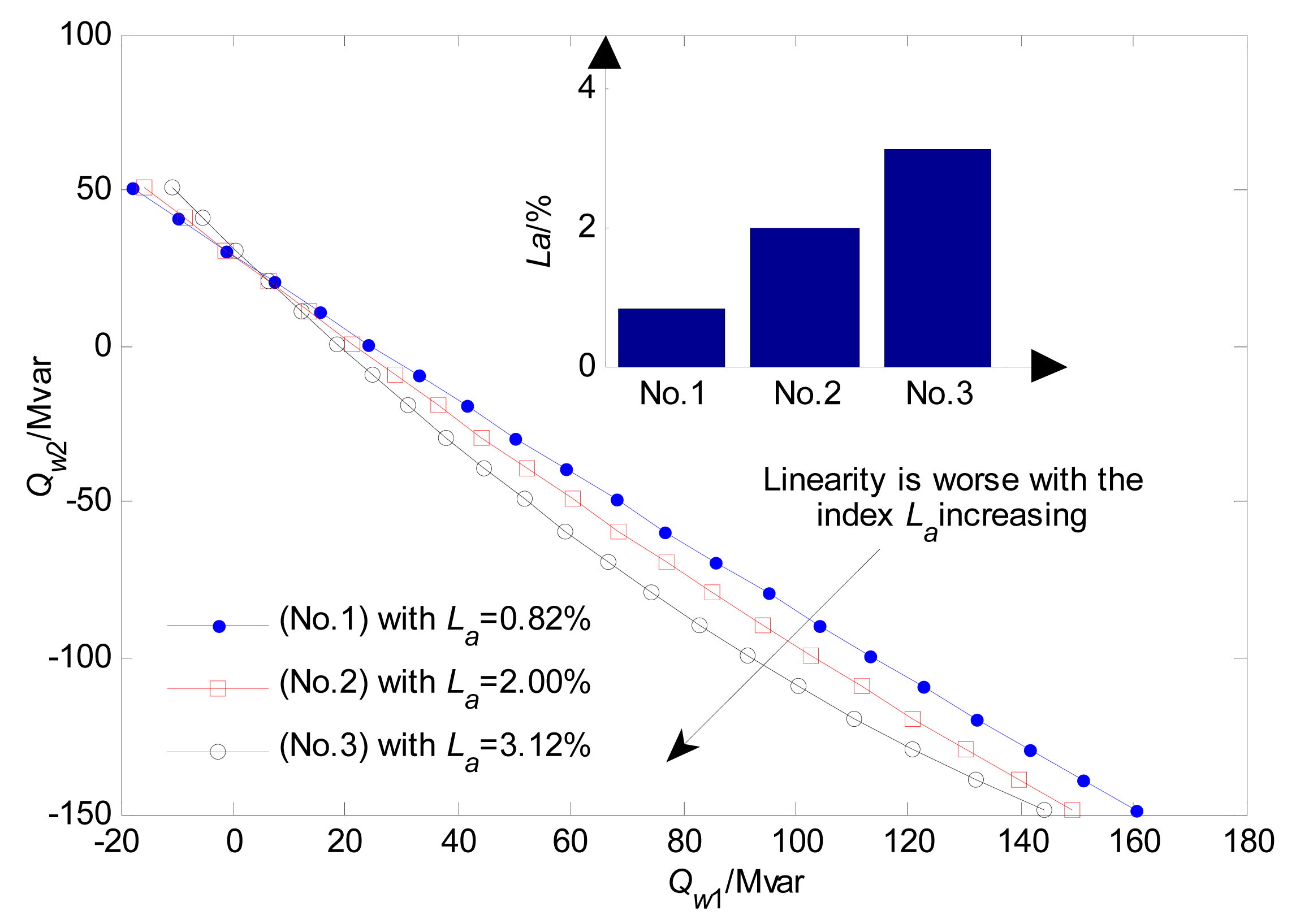
In the previous section, a linearity index was proposed to measure how well nonlinear boundary curves can be approximated by linear counterparts.

Table 1. Line parameters (p.u.) with corresponding PCC voltages and values of the linearity index

Parameter Set		R (p.u.)	X (p.u.)	B (p.u.)	PCC Voltage (p.u.)	Index La
1	w1	0.003	0.018	0.126	1.091 (0.902)	0.82% (0.22%)
	w2	0.005	0.028	0.111
2	w1	0.010	0.055	0.142	1.078 (0.901)	2.00% (0.11%)
	w2	0.012	0.064	0.126
3	w1	0.017	0.092	0.158	1.065 (0.902)	3.12% (0.22%)
	w2	0.017	0.092	0.158

Note: Both the voltage magnitude and the linearity index have two values, one at each of the two near points. The value in parentheses is the value at near point T₃ (i.e., ξ⁻), and the other value is the value at near point T₁ (i.e., ξ⁺).

lists the values of the linearity index for different sets of resistances and reactances between the wind farms and the PCC, while Figure 8 shows the corresponding nonlinear boundary curves, obtained using the sampling-based approach. Both Table 1 and Figure 8 indicate that the linearity near point T₁ (i.e., ξ⁺) deteriorates with increasing line resistance and reactance, while the linearity near point T₃ (i.e., ξ⁻) exhibits a similar pattern. We use line parameter set No. 3 in the following simulation to represent a worst-case scenario.

3.2. Linear Approximation of Ω_S

In Section II, four approximation techniques were introduced. Among these, the techniques of Figure 6c,d are the most promising because they yield approximate security regions that span most of the actual security regions, and require only a limited number of additional computations. These two techniques are compared in the present section.

For the linear approximation technique of Figure 6c, tangent planes at the near points are required. To calculate these, the Jacobian matrices at the two respective near points were calculated first as follows. Thus, the tangent planes (denoted by ∇) can be written as:

$$\nabla =\{\begin{array}{l}0.0401Q_{w1}+0.0257Q_{w2}=1\\ 0.0242Q_{w1}+0.0357Q_{w2}=1\\ 0.0270Q_{w1}+0.0196Q_{w2}=-1\\ 0.0212Q_{w1}+0.0265Q_{w2}=-1\end{array}$$

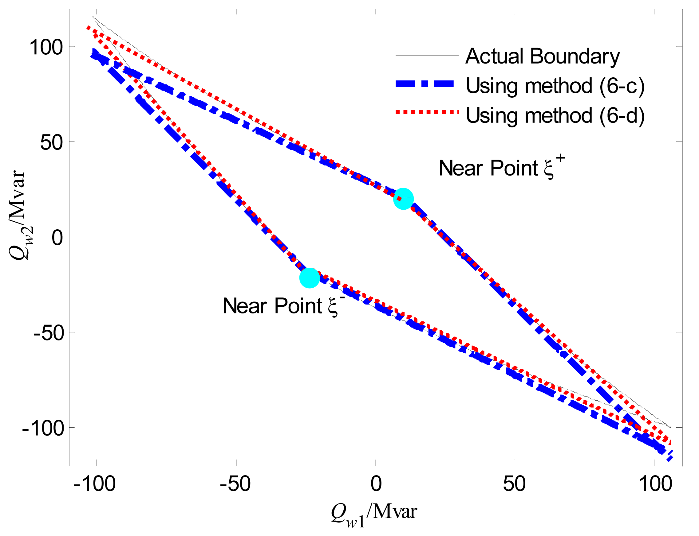
For the linear approximation technique of Figure 6d, inner points are required to construct the cutting planes. The calculated inner points near ξ⁺ (i.e., T₁) were (25.25, 0) and (0, 28.19). The inner points near ξ⁻ (i.e., T₃) were (−36.43, 0) and (0, −36.72). Utilizing the inner points and near points, the coefficients of the cutting planes were calculated as follows:

$$\mathrm{\Delta }=\{\begin{array}{l}0.0396Q_{w1}+0.0260Q_{w2}=1\\ 0.0245Q_{w1}+0.0355Q_{w2}=1\\ 0.0274Q_{w1}+0.0191Q_{w2}=-1\\ 0.0205Q_{w1}+0.0272Q_{w2}=-1\end{array}$$

The linear boundary components formed by the tangent planes and the cutting planes, together with the actual boundary, are shown in Figure 9, which suggest that the technique of Figure 6d provides a better linear approximation to the actual boundary of the security region than that of Figure 6c. The drawback of the technique of Figure 6d is that it employs two inner points, and thus requires the calculation of m² (= m × m) additional power flows and the inverses of m m × m matrices in order to construct the cutting planes. In this example, m = 2.

3.3. Final Voltage Security Region (Ω_VSR)

Assume that the power factor of each wind farm ranges from capacitive 0.90 to inductive 0.90. The corresponding reactive power limits are:

$$\{\begin{array}{l}-38.7458\le Q_{w1}\le 38.7458\\ -77.4916\le Q_{w2}\le 77.4916\end{array}$$

With these reactive power limits, the initial security region of Figure 3 changes to the final security region, represented by the shaded area in Figure 10.

Note that both near points remain in the final voltage security region Ω_VSR, while both remote points are outside Ω_VSR. In addition, the final bounds on w₁ are determined by its reactive power limits, whereas the original reactive power limits of wind farm w₂ lie completely outside the final voltage security region. This indicates that simply operating under the reactive power limits cannot guarantee voltage security. It should be noted that the shape of the final voltage security region can change with the power factors. With higher power factors, more stringent reactive power limits are imposed, and hence more boundary components of the final security region can be determined by the reactive power limits.

3.4. A Practical Large System Simulation

Furthermore, we take a practical 12-wind-farm system in Zhangbei wind base in Northeast China. The wind farm parameters are given as Table 1, where the external grid is chosen as the standard IEEE 118-bus system and the PCC bus is #114. The topology of wind farms are shown in Figure 11, and the parameters can be found in Appendix III.

According to the proposed method, the cutting planes can be calculated using the inner points and near points, as follows:

$$\mathrm{\Delta }:\left(\begin{array}{cccccccccccc}0.1139& 0.0632& 0.0630& 0.0632& 0.0633& 0.0632& 0.0631& 0.0633& 0.0632& 0.0632& 0.0632& 0.0632\\ 0.0624& 0.1279& 0.0622& 0.0624& 0.0624& 0.0623& 0.0622& 0.0624& 0.0623& 0.0623& 0.0623& 0.0623\\ 0.0468& 0.0468& 0.3421& 0.0468& 0.0469& 0.0468& 0.0467& 0.0469& 0.0468& 0.0468& 0.0468& 0.0468\\ 0.0630& 0.0630& 0.0628& 0.1135& 0.0630& 0.0630& 0.0629& 0.0630& 0.0630& 0.0630& 0.0630& 0.0630\\ 0.0649& 0.0649& 0.0647& 0.0649& 0.0837& 0.0648& 0.0649& 0.0649& 0.0649& 0.0648& 0.0649& 0.0649\\ 0.0612& 0.0612& 0.0610& 0.0612& 0.0612& 0.1537& 0.0611& 0.0612& 0.0612& 0.1462& 0.0623& 0.0624\\ 0.0499& 0.0499& 0.0497& 0.0499& 0.0499& 0.0498& 0.2997& 0.0499& 0.0499& 0.0498& 0.0498& 0.0498\\ 0.0649& 0.0649& 0.0647& 0.0649& 0.0649& 0.0649& 0.0648& 0.0837& 0.0649& 0.0649& 0.0648& 0.0649\\ 0.0630& 0.0630& 0.0628& 0.0630& 0.0630& 0.0630& 0.0629& 0.0630& 0.1135& 0.0630& 0.0630& 0.0630\\ 0.0624& 0.0624& 0.0622& 0.0624& 0.0624& 0.0624& 0.0623& 0.0624& 0.0624& 0.1462& 0.0623& 0.0624\\ 0.0603& 0.0603& 0.0601& 0.0603& 0.0603& 0.0603& 0.0602& 0.0603& 0.0603& 0.0603& 0.1513& 0.0603\\ 0.0598& 0.0598& 0.0596& 0.0598& 0.0598& 0.0598& 0.0597& 0.0598& 0.0598& 0.0598& 0.0598& 0.1584\end{array}\right)\left(\begin{array}{l}{Q}_{w,1}\\ Q_{w,2}\\ Q_{w,3}\\ Q_{w,4}\\ Q_{w,5}\\ Q_{w,6}\\ Q_{w,7}\\ Q_{w,8}\\ Q_{w,9}\\ Q_{w,10}\\ Q_{w,11}\\ Q_{w,12}\end{array}\right)=\left(\begin{array}{l}1\\ 1\\ 1\\ 1\\ 1\\ 1\\ 1\\ 1\\ 1\\ 1\\ 1\\ 1\end{array}\right)$$

$$\mathrm{\Delta }:\left(\begin{array}{cccccccccccc}0.1229& 0.0658& 0.0648& 0.0658& 0.0659& 0.0656& 0.0651& 0.0660& 0.0658& 0.0657& 0.0655& 0.0656\\ 0.0648& 0.1344& 0.0638& 0.0648& 0.0649& 0.0646& 0.0641& 0.0650& 0.0649& 0.0647& 0.0645& 0.0646\\ 0.0484& 0.0484& 0.3568& 0.0484& 0.0485& 0.0482& 0.0478& 0.0485& 0.0484& 0.0483& 0.0482& 0.0482\\ 0.0660& 0.0660& 0.0650& 0.1233& 0.0662& 0.0658& 0.0653& 0.0662& 0.0661& 0.0660& 0.0657& 0.0658\\ 0.0688& 0.0689& 0.0678& 0.0689& 0.0891& 0.0687& 0.0681& 0.0690& 0.0689& 0.0688& 0.0685& 0.0687\\ 0.0621& 0.0622& 0.0612& 0.0622& 0.0623& 0.1598& 0.0615& 0.0623& 0.0622& 0.0621& 0.0619& 0.0620\\ 0.0519& 0.0519& 0.0511& 0.0519& 0.0520& 0.0517& 0.3097& 0.0520& 0.0519& 0.0518& 0.0516& 0.0517\\ 0.0688& 0.0689& 0.0678& 0.0689& 0.0690& 0.0687& 0.0681& 0.0891& 0.0689& 0.0688& 0.0685& 0.0687\\ 0.0660& 0.0660& 0.0650& 0.0660& 0.0662& 0.0658& 0.0653& 0.0662& 0.1234& 0.0660& 0.0657& 0.0658\\ 0.0622& 0.0622& 0.0613& 0.0622& 0.0623& 0.0620& 0.0615& 0.0623& 0.0623& 0.1513& 0.0619& 0.0620\\ 0.0615& 0.0615& 0.0606& 0.0615& 0.0617& 0.0613& 0.0608& 0.0617& 0.0616& 0.0615& 0.1832& 0.0613\\ 0.0623& 0.0623& 0.0614& 0.0623& 0.0624& 0.0621& 0.0616& 0.0624& 0.0623& 0.0622& 0.0620& 0.1729\end{array}\right)\left(\begin{array}{l}{Q}_{w,1}\\ Q_{w,2}\\ Q_{w,3}\\ Q_{w,4}\\ Q_{w,5}\\ Q_{w,6}\\ Q_{w,7}\\ Q_{w,8}\\ Q_{w,9}\\ Q_{w,10}\\ Q_{w,11}\\ Q_{w,12}\end{array}\right)=\left(\begin{array}{l}-1\\ -1\\ -1\\ -1\\ -1\\ -1\\ -1\\ -1\\ -1\\ -1\\ -1\\ -1\end{array}\right)$$

With twelve wind farms, the initial voltage security region is a high-dimensional space. For illustrative purposes, the projection of this twelve-dimensional space on the (Q_w1, Q_w2) and (Q_w5, Q_w8)-plane are shown in Figure 12a,c which are represented by the shaded area respectively. Similarly, the final voltage security region with the consideration of the reactive power limits are shown in Figure 12b,d. The comparison between initial and final voltage security region shows that the remote points may be cut off due to the reactive power limit.

4. Conclusions

This paper has proposed for the first time the concept of a voltage security region, and described a sampling-based approach for obtaining it and its nonlinear boundary components. Several different linear approximation techniques were presented and compared. One of these is expected to produce an approximate security region that is very close to the actual one, and can be easily represented in closed mathematical form, while greatly reducing the required computations. The simulation results verified the effectiveness of the proposed method. The proposed voltage security region is the basis for an N-1 voltage security region to provide better coordination among wind farms and help prevent cascading tripping when a single wind farm is tripped. Further analysis on the voltage security region under N-1 contingencies will be presented in Part II [24].

References

- Momoh, J.A. Electric Power Distribution, Automation, Protection and Control; CRC Press: Boca Raton, FL, USA, 2007; pp. 223–230. [Google Scholar]
- Wind Power. Available online: http://en.wikipedia.org/wiki/Wind_power (accessed on 26 November 2013).
- Sideratos, G.; Hatziargyriou, N.D. An advanced statistical method for wind power forecasting. IEEE Trans. Power Syst. 2007, 22, 258–265. [Google Scholar]
- Soder, L. Reserve margin planning in a wind-hydro-thermal power system. IEEE Trans. Power Syst. 1993, 8, 564–571. [Google Scholar]
- Doherty, R.; Denny, E.; O'Malley, M. System Operation with a Significant Wind Power Penetration. Proceedings of the IEEE Power Engineering Society General Meeting, Denver, CO, USA, 6–10 June 2004; Volume 1, pp. 1002–1007.
- Morales, J.M.; Conejo, A.J.; Perez-Ruiz, J. Economic valuation of reserve in power systems with high penetration of wind power. IEEE Trans. Power Syst. 2009, 24, 900–910. [Google Scholar]
- Ilic, M.D.; Xie, L.; Joo, J.Y. Efficient coordination of wind power and price-responsive demand—Part I: Theoretical foundations. IEEE Trans. Power Syst. 2011, 26, 1875–1884. [Google Scholar]
- Burchett, R.C.; Heydt, G.T. Probabilistic methods for power system dynamic stability studies. IEEE Trans. Power App. Syst. 1978, 97, 695–702. [Google Scholar]
- Chung, C.Y.; Wang, K.W.; Tse, C.T.; Bian, X.Y.; David, A.K. Probabilistic eigenvalue sensitivity analysis and PSS design in multi-machine systems. IEEE Trans. Power Syst. 2003, 18, 1439–1445. [Google Scholar]
- Yi, H.Q.; Hou, Y.H.; Cheng, S.J.; Zhou, H.; Chen, G.G. Power System Probabilistic Small Signal Stability Analysis Using Two Point Estimation Method. Proceedings of the 42nd International Universities Power Engineering Conference, Brighton, UK, 4–6 September 2007; pp. 402–407.
- Bu, S.Q.; Du, W.; Wang, H.F.; Chen, Z.; Xiao, L.Y.; Li, H.F. Probabilistic analysis of small-signal stability of large-scale power systems as affected by penetration of wind generation. IEEE Trans. Power Syst. 2012, 27, 762–770. [Google Scholar]
- Vittal, E.; Keane, A.; O'Malley, M. Varying Penetration Ratios of Wind Turbine Technology for Voltage and Frequency Stability. Proceedings of the IEEE Power and Energy Society General Meeting—Conversion and Deliver of Electrical Energy in the 21st Century, Pittsburgh, PA, USA, 20–24 July 2008; pp. 1–6.
- Vittal, E.; O'Malley, M.; Keane, A. Impact of Wind Turbine Control Strategies on Voltage Performance. Proceedings of the IEEE Power and Energy Society General Meeting (PES), Calgary, AB, Canada, 26–30 July 2009; pp. 1–7.
- Vittal, E.; O'Malley, M.; Keane, A. A steady-state voltage stability analysis of power systems with high penetrations of wind. IEEE Trans. Power Syst. 2010, 25, 433–442. [Google Scholar]
- Palsson, M.P.; Toftevaag, T.; Uhlen, K.; Tande, J.O.G. Large-Scale Wind Power Integration and Voltage Stability Limits in Regional Networks. Proceedings of the IEEE Power Engineering Society Summer Meeting, Chicago, IL, USA, 21–25 July 2002; pp. 762–769.
- Zhou, F.Q.; Joos, G.; Abbey, C. Voltage Stability in Weak Connection Wind Farms. Proceedings of the IEEE Power Engineering Society General Meeting, San Francisco, CA, USA, 12–16 June 2005; pp. 1483–1488.
- Abbey, C.; Joos, G. Effect of Low Voltage Ride Through (LVRT) Characteristic on Voltage Stability. Proceedings of the IEEE Power Engineering Society General Meeting, San Francisco, CA, USA, 12–16 June 2005; pp. 1901–1907.
- Linh, N.T. Voltage Stability Analysis of Grids Connected Wind Generators. Proceedings of the 4th IEEE Conference on Industrial Electronics and Applications (ICIEA), Xi'an, China, 25–27 May 2009; pp. 2657–2660.
- McCalley, J.D.; Wang, S.; Zhao, Q.-L.; Zhou, G.; Treinen, R.T.; Papalexopoulos, A.D. Security boundary visualization for systems operation. IEEE Trans. Power Syst. 1997, 12, 940–947. [Google Scholar]
- Su, J.F.; Yu, Y.X.; Jia, H.J.; Li, P.; He, N.Q.; Tang, Z.Y.; Fu, H.J. Visualization of Voltage Stability Region of Bulk Power System. Proceedings of the International Conference on Power System Technology, Kunming, China, 13–17 October 2002; pp. 1665–1668.
- Wei, W.; Zhang, P.; Min, L.; Graham, M.; Ramsay, D. Voltage Stability Margin Computation and Visualization for Tri-State South Colorado area Using EPRI Power System Voltage Stability Region (PSVSR) Program. Proceedings of the Asia-Pacific Power and Energy Engineering Conference, Wuhan, China, 27–31 March 2009; pp. 1–6.
- Dong, Z.Y.; Miao, W.W.; Jia, H.J. Minimum Load Shedding Calculation Based on Static Voltage Security Region in Load Injection Space. Proceedings of the Region 10 Conference (TENCON), Bali, Indonesia, 21–24 November 2011; pp. 959–963.
- Lee, S.T. Community Activity Room as a New Tool for Transmission Operation and Planning under a Competitive Power Market. Proceedings of the 2003 IEEE Bologna Power Tech Conference, Bologna, Italy, 23–26 June 2003.
- Ding, T.; Guo, Q.; Bo, R.; Sun, H.; Zhang, B.; Huang, T. A static voltage security region for centralized wind power integration—Part II: Applications. Energies 2014, 7, 444–461. [Google Scholar]
- Yue, X.N.; Venkatasubramanian, V. Complementary Limit Induced Bifurcation Theorem and Analysis of Q Limits in Power-Flow Studies. Proceedings of the Bulk Power System Dynamics and Control-VII. Revitalizing Operational Reliability (2007 IREP Symposium), Charleston, SC, USA, 19–24 August 2007; pp. 1–8.
- MATPOWER. Available online: http://www.pserc.cornell.edu/matpower/ (accessed on 26 November 2013).
Nomenclature