A Real-Time Sliding Mode Control for a Wind Energy System Based on a Doubly Fed Induction Generator

Abstract

In this paper, a real time sliding mode control scheme for a variable speed wind turbine that incorporates a doubly feed induction generator is described. In this design, the so-called vector control theory is applied, in order to simplify the system electrical equations. The proposed control scheme involves a low computational cost and therefore can be implemented in real-time applications using a low cost Digital Signal Processor (DSP). The stability analysis of the proposed sliding mode controller under disturbances and parameter uncertainties is provided using the Lyapunov stability theory. A new experimental platform has been designed and constructed in order to analyze the real-time performance of the proposed controller in a real system. Finally, the experimental validation carried out in the experimental platform shows; on the one hand that the proposed controller provides high-performance dynamic characteristics, and on the other hand that this scheme is robust with respect to the uncertainties that usually appear in the real systems.

1. Introduction

Since the late 1990s wind power has experienced a rapid global growth. This high growth rate of wind power capacity is explained by the cost reduction as well as by new public government subsides in many countries linked to efforts to increase the use of renewable power production and reduce CO₂ emissions.

The new worldwide wind annual installed capacity has increased by 35.47 GW in 2013, which is significantly less that the 44.56 GW of the year 2012. The total installed wind capacity reached 318.14 GW by the end of the year 2013, enough to provide almost 4% of the global electricity demand, taking into account the capacity factor of the wind power plants [1]. The year 2013 has been a difficult year for the wind industry worldwide as the companies have to struggle with a decreasing market size. This situation has already led to decrease in wind turbine prices which will make wind power even more cost competitive [1]. This expected decrease in new installations is mainly due to the abnormal situation due to the finance crisis, so although we currently face some challenges, we are still confident about wind power development in the future. Hence, it can be expected that the wind markets worldwide will be able to recover from the 2013 decrease and set a new record in the year 2014, because in spite of the need to reinforce national and international policies and to accelerate the deployment of wind power, it can be observed that appetite for investment in wind power is strong and many projects are in the pipeline.

The World Wind Energy Association (WWEA) expects that wind energy will continue its dynamic development in the coming years. Although the short term impacts of the current finance crisis makes short-term predictions rather difficult, it can be expected that in the mid-term wind energy will rather attract more investors due to its low risk character and the need for clean and reliable energy sources. More and more governments understand the manifold benefits of wind energy and are setting up favorable policies, including those that are stimulation decentralized investment by independent power producers, small and medium sized enterprises and community based projects, all of which will be main drivers for a more sustainable energy system also in the future.

Further substantial growth can especially be expected in China, India, Europe and North America. High growth rates can be expected in several Latin American countries, in particular in Brazil, as well as in new Asian and Eastern European markets. In the mid-term, also some of the African countries will see major investment, mostly in northern Africa, but also in South Africa.

However, taking into account some insecurity factors and based on the current growth rates, the WWEA revises its expectations for the future growth of the global wind capacity. In 2016, the global capacity of 500 GW is possible. By the end of year 2020, at least 1000 GW of installed capacity can be expected globally.

Nevertheless, large wind power penetration faces a variety of technical problems and challenges such as frequency and voltage regulation, power quality issues, electromagnetic interference, etc. that should be addressed in order to further increase the wind power penetration [2–4].

The doubly Feed Induction Generator (DFIG) is widely used in variable speed wind turbine systems owing to their ability to maximize wind power extraction and to their capability to fulfill the basic technical requirements set by the system operators and contribute to power system security [5–9]. In these DFIG wind turbines the control system should be designed in order to achieve the following objectives: regulating the DFIG rotor speed for maximum wind power capture, maintaining the DFIG stator output voltage frequency constant and controlling the DFIG reactive power [10].

One of the main task of the controller is to carry the turbine rotor speed into the desired optimum speed in order to extract the maximum active power from the wind. This is a difficult task because there are system uncertainties and the wind speed varies over time [11–13].

This paper proposes a robust control scheme for a Wind Turbine System (WTS) equipped with a DFIG. The proposed robust design uses the sliding mode control algorithm to regulate both the rotor-side converter (RSC) and the grid-side converter (GSC). In the design, a vector oriented control theory is used in order to decouple the torque and the flux of the induction machine. This control scheme leads to obtain the maximum power extraction from the different wind speeds that appear along the time. The proposed controller is based on the control scheme proposed in [14]; however, in this paper, real time control experiments are developed and the sliding mode controllers has been modified in order to improve the real time performance of these controllers. In this sense, the sliding variable has been modified in order to simplify it, and the saturation function has been replace by a hyperbolic tangent function in order to simplify it. These simplifications improve the real time performance of the controller.

A new experimental platform has been designed and constructed in order to show the real performance of the proposed control scheme over a real system. The control platform that we have designed and constructed is formed by a PC with MatLab7/Simulink R2007a, dsControl 3.2.1 and the DS1103 Controller Board real time interface of dSpace. The electric machine used to implement the proposed controller is a commercial machine of Leroy Somer of 7.5 kW, 1447 rpm, double feed induction machine connected to the grid through the rotor in a Back to Back configuration with two voltage source inverters. The wind profiles are generated by a 10.6 kW 190U2 Unimotor synchronous AC servo motor. In this platform several test have been made using different operating conditions and satisfactory results are obtained.

2. System Modeling

The power extraction of a wind turbine is a function of three main factors: the wind power available, the power curve of the machine and the ability of the machine to respond to wind fluctuation. The expression for power produced by the wind is given by [15]:

$$P_m(v)=\frac{1}{2}{C}_p(\lambda ,\beta )\rho \pi R^2{v}^3$$

(1)

where ρ is the air density; R is the radius of turbine blades; v is the wind speed; C_p denotes the power coefficient of the wind turbine; λ is the tip-speed ratio and β represents the pitch angle.

The tip-speed ratio is defined as:

$$\lambda =\frac{R{w}_m}{v}$$

(2)

where w_m is the turbine rotor speed. Therefore, if the rotor speed is kept constant, then any change in the wind speed will change the tip-speed ratio, leading to the change of power coefficient C_p, as well as the generated power output of the wind turbine. However, if the rotor speed is adjusted according to the wind speed variation, then the tip-speed ratio can be maintained at an optimal point, which could yield maximum power output from the system.

The WTS primarily consists of an aeroturbine, which converts wind energy into mechanical energy, a gearbox, which serves to increase the speed and decrease the torque and a generator used to convert the mechanical energy into the electrical energy.

Driven by the input wind torque T_m, the rotor of the wind turbine runs at the speed w_m. This mechanical torque is the input to the electrical generator, which generates the electrical torque T_e at the generator angular velocity w. Note that turbine speed and generator speed are not the same in general, due to the use of the gearbox.

The relation between the angular velocity of the turbine w_m and the angular velocity of the generator w is given by the gear ratio γ:

$$\gamma =\frac{w_m}{w}$$

(3)

The Wind Turbine system mechanical equations can be represented by [14]:

$$J\dot{w}+Bw=\gamma T_m+T_e$$

(4)

with

$$J={\gamma }^2{J}_m+J_e$$

(5)

$$B={\gamma }^2{B}_m+B_e$$

(6)

where J_m and J_e are the momentum of inertia of the turbine and the generator; B_m and B_e are the viscous friction coefficient of the the turbine and the generator; T_m is the mechanical torque generated in the wind turbine; T_e is the torque produced in the electrical generator.

Using Equations (1) and (2) the input wind torque can be calculated by:

$$T_m(v)=\frac{P_m(v)}{w_m}=\frac{P_m(v)}{\frac{\lambda v}{R}}=k_v\cdot v^2$$

(7)

where

$$k_v=\frac{1}{2}{C}_p(\lambda ,\beta )\rho \pi \frac{R^3}{\lambda }$$

(8)

Now, let us consider the system electrical equations. In this work a double feed induction generator (DFIG) is used. This induction machine is feed from both stator and rotor sides. The stator is directly connected to the grid while the rotor is fed through a variable frequency converter (VFC). In order to produce electrical active power at constant voltage and frequency to the utility grid, over a wide operation range (from subsynchronous to supersynchronous speed), the active power flow between the rotor circuit and the grid must be controlled both in magnitude and in direction. Therefore, the VFC consists of two four-quadrant IGBT PWM converters, the rotor-side converter (RSC) and the grid-side converter (GSC) that are connected back-to-back by a dc-link capacitor [16].

The DFIG can be regarded as a traditional induction generator with a nonzero rotor voltage. The dynamic equation of a thee-phase DFIG can be written in a synchronously rotating d-q reference frame as [17]:

$$v_{ds}=r_s{i}_{ds}-w_s{\psi }_{qs}+\frac{d{\psi }_{ds}}{dt}$$

(9)

$$v_{qs}=r_s{i}_{qs}+w_s{\psi }_{ds}+\frac{d{\psi }_{qs}}{dt}$$

(10)

$$v_{dr}=r_r{i}_{dr}-s{w}_s{\psi }_{qr}+\frac{d{\psi }_{dr}}{dt}$$

(11)

$$v_{qs}=r_r{i}_{qr}+s{w}_s{\psi }_{dr}+\frac{d{\psi }_{qr}}{dt}$$

(12)

where w_s is the rotational speed of the synchronous reference frame; sw_s = w_s − w_e is the slip frequency and s is the slip; w_e is the generator electrical speed, that is related to the generator mechanical speed by mean of the pole numbers $w_e=\frac{p}{2}w$; and ψ is the flux.

The electrical torque for the DFIG is can be calculated by:

$$T_e=\frac{3p}{4}{L}_m(i_{qs}{i}_{dr}-i_{ds}{i}_{qr})$$

(13)

where p is the pole numbers.

The active and reactive stator powers for the DFIG are:

$$P_s=\frac{3}{2}(v_{ds}{i}_{ds}+v_{qs}{i}_{qs})$$

(14)

$$Q_s=\frac{3}{2}(v_{qs}{i}_{ds}-v_{ds}{i}_{qs})$$

(15)

where the power loses associated with the stator resistances are neglected.

Similarly, the rotor active and reactive powers (also called slip power) can be calculated as:

$$P_r=\frac{3}{2}(v_{dr}{i}_{dr}+v_{qr}{i}_{qr})$$

(16)

$$Q_r=\frac{3}{2}(v_{qr}{i}_{dr}-v_{dr}{i}_{qr})$$

(17)

where the power loses associated with the rotor resistances are also neglected.

Finally, the total active power P_e and reactive power Q_e injected into the grid are:

$$P_e=P_s+P_r$$

(18)

$$Q_e=Q_s+Q_r$$

(19)

where the power losses in the converters are neglected.

3. Wind Turbine Control Scheme

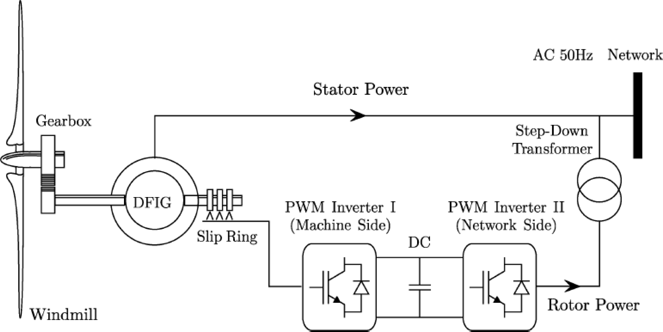
The control of the DFIG is achieved by controlling the variable frequency converter (VFC), which includes control of the rotor side converter (RSC) and control of the grid side converter (GSC). The objective of the RSC is to govern both the stator-side active and reactive powers independently. On the other hand, the objective of the GSC is to keep the dc-link voltage constant regardless of the magnitude and direction of the rotor power. The GSC control scheme can also be designed to regulate the reactive power or the stator terminal voltage of the DFIG. A typical scheme of a DFIG equipped wind turbine is shown in Figure 1.

When the WTS operates in the variable-speed mode, in order to extract the maximum active power from the wind, the shaft speed of the WTG must be adjusted to achieve an optimal tip-speed ratio λ_opt, which yields the maximum power coefficient C_pmax, and therefore the maximum power [18]. In other words, given a particular wind speed, there is a unique wind turbine speed command to achieve the goal of maximum wind power extraction. The value of the λ_opt can be calculated from the maximum of the power coefficient curves versus tip-speed ratio.

The power coefficient C_p, can be approximated by Equation (20) [19]:

$$C_p(\lambda ,\beta )=c_1\left(\frac{c_2}{{\lambda }_1}-c_3\beta -c_4\right)e^{\frac{-c_5}{{\lambda }_i}}+c_6\lambda$$

(20)

where the coefficients c₁ to c₆ depends on the wind turbine design characteristics, and λ_i is defined as

$$\frac{1}{{\lambda }_i}=\frac{1}{\lambda +0.08\beta }-\frac{0.035}{{\beta }^3+1}$$

(21)

The value of λ_opt can be obtained from Equation (20) calculating the λ value that maximizes the power coefficient. Then, based on the wind speed, the corresponding optimal generator speed command for maximum wind power extraction is determined by:

$$w_m^{*}=\frac{{\lambda }_{\mathit{opt}}\cdot v}{R}$$

(22)

4. Wind Turbine Speed Control

The objective of the maximum wind power extraction can be achieved using an adequate speed controller that regulates the wind turbine speed in order to get the reference speed $w_m^{*}$ that gives the optimal tip-speed ratio λ_opt. In the DFIG based wind generation system, this objective is commonly achieved by means of the rotor current regulation in the electrical generator. This current regulation is usually performed by the RSC control, using the stator-flux oriented reference frame in order to simplify the DFIG dynamic equations.

In the stator-flux oriented reference frame, the d-axis is aligned with the stator flux linkage vector ψ_s, and then, ψ_ds = ψ_s and ψ_qs = 0. This yields the following relationships [20]:

$$i_{qs}=-\frac{L_m{i}_{qr}}{L_s}$$

(23)

$$i_{ds}=\frac{L_m(i_{ms}-i_{dr})}{L_s}$$

(24)

$$i_{ms}=\frac{v_{qs}-r_s{i}_{qs}}{w_s{L}_m}$$

(25)

$$T_e=-\frac{3p}{4}\frac{L_m^2{i}_{ms}{i}_{qr}}{L_s}$$

(26)

$$Q_s=\frac{3}{2}\frac{w_s{L}_m^2{i}_{ms}(i_{ms}-i_{dr})}{L_s}$$

(27)

$$v_{dr}=r_r{i}_{dr}+\sigma L_r\frac{d{i}_{qr}}{dt}-s{w}_s\sigma L_r{i}_{qr}$$

(28)

$$v_{qr}=r_r{i}_{qr}+\sigma L_r\frac{d{i}_{qr}}{dt}+s{w}_s\left(\sigma L_r{i}_{dr}+\frac{L_m^2{i}_{ms}}{L_s}\right)$$

(29)

where $\sigma =1-\frac{L_m^2}{L_s{L}_r}$

Since the stator is connected to the grid, and the influence of the stator resistance is small, the stator magnetizing current (i_ms) can be considered constant [16]. Therefore, the electromagnetic torque can be defined as follows:

$$T_e=-K_T{i}_{qr}$$

(30)

where K_T is a torque constant, and is defined as follows:

$$K_T=\frac{L_m{i}_{ms}}{L_s}$$

(31)

From the previous Equations (4) and (30) it is obtained that regulating the q-component of the rotor current (i_qr), the wind turbine speed can be controlled.

Then, the following dynamic equation for the system speed is obtained using Equations (4) and (30):

$$\dot{w}=\frac{1}{J}\left(\gamma T_m-K_T{i}_{qr}-Bw\right)=-aw+f-b{i}_{qr}$$

(32)

where the parameters are defined as:

$$a=\frac{B}{J},\hspace{0.17em}\hspace{0.17em}\hspace{0.17em}\hspace{0.17em}\hspace{0.17em}b=\frac{K_T}{J},\hspace{0.17em}\hspace{0.17em}\hspace{0.17em}\hspace{0.17em}f=\frac{\gamma T_m}{J};$$

(33)

In order to take into account the system uncertainties the previous dynamic Equation (32) are modified to:

$$\dot{w}=-(a+\mathrm{\Delta }a)w+(f+\mathrm{\Delta }f)-(b+\mathrm{\Delta }b)i_{qr}$$

(34)

where the terms Δa, Δb and Δf represents the uncertainties of the terms a, b and f respectively.

The dynamic Equation (34) can be rewritten as:

$$\dot{w}=-aw+f-b{i}_{qr}+d(t)$$

(35)

where the he signal d(t) collets the uncertainty terms and is defined as:

$$d(t)=-\mathrm{\Delta }aw(t)+\mathrm{\Delta }f(t)-\mathrm{\Delta }b\hspace{0.17em}\hspace{0.17em}{i}_{qr}(t)$$

(36)

In this paper, a sliding mode control scheme is proposed in order to compensate for the above described uncertainties.

The speed tracking error is defined as follows:

$$e(t)=w(t)-w^{*}(t)$$

(37)

where

$$w^{*}=\frac{w_m^{*}}{\gamma }$$

(38)

is the generator speed command that provides the optimum tip speed ratio.

Taking the derivative of the previous equation with respect to time yields:

$$\dot{e}(t)=\dot{w}-{\dot{w}}^{*}=-aw(t)+f(t)-b{i}_{qr}+d(t)-{\dot{w}}^{*}$$

(39)

The sliding variable S (t) is defined as:

$$S(t)=e(t)+{\int }_0^{t}ke(\tau )d\tau$$

(40)

where k is a positive constant gain.

The wind turbine speed can be regulated by means of the q-component of the rotor current i_qr. In this sense, a sliding mode controller is proposed in order to control the q-component of the rotor current:

$$i_{qr}(t)=\frac{1}{b}\left[+ke(t)+\beta sgn(S)+f(t)-aw(t)-{\dot{w}}^{*}\right]$$

(41)

where the k is the constant gain defined previously; β ≥ |d(t)| is the switching gain that should be chosen greater than the system uncertainties; S is the sliding variable defined in Equation (40) and sgn(·) is the sign function.

The control law Equation (41) regulates the wind turbine generator speed w(t), so that the speed tracking error e(t) = w(t) − w^*(t) tends to zero as the time tends to infinity.

Proof : Define the Lyapunov function candidate:

$$V(t)=\frac{1}{2}S(t)S(t)$$

(42)

The time derivative of the Lyapunov function candidate is calculated as:

$$\begin{array}{lll}\dot{V}(t)\hfill & =\hfill & S(t)\dot{S}(t)\hfill \\ \hfill & =\hfill & S\cdot [\dot{e}+ke]\hfill \\ \hfill & =\hfill & S\cdot \left[-aw+f-{\mathit{bi}}_{qr}+d-{\dot{w}}^{*}+ke\right]\hfill \\ \hfill & =\hfill & S\cdot \left[-aw+f-ke-\beta sgn(S)-f+aw+{\dot{w}}^{*}+d-{\dot{w}}^{*}+ke\right]\hfill \\ \hfill & =\hfill & S\cdot \left[d-\beta sgn(S)\right]\hfill \\ \hfill & \le \hfill & -\left(\beta -\left|d\right|\right)\left|S\right|\hfill \\ \hfill & \le \hfill & 0\hfill \end{array}$$

(43)

It should be noted that the Equations (39)–(41) have been used in the proof.

Using the Lyapunov’s direct method, since V(t) is clearly positive-definite, V̇(t) is negative definite and V(t) tends to infinity as S (t) tends to infinity, then the equilibrium at the origin S (t) = 0 is globally asymptotically stable. Therefore S (t) tends to zero as the time tends to infinity. Moreover, all trajectories starting off the sliding surface S = 0 must reach it in finite time and then will remain on this surface. This system’s behavior once on the sliding surface is usually called sliding mode [21].

When the sliding mode occurs on the sliding surface then S (t) = Ṡ (t) = 0, and therefore the dynamic behavior of the tracking problem Equation (39) is equivalently governed by the following Equation:

$$\dot{S}(t)=0\Rightarrow \dot{e}(t)=-ke(t)$$

(44)

Then, the tracking error e(t) converges to zero exponentially.

A frequently encountered problem in the sliding control is that the control signal given by Equation (41) is quite abrupt since the sliding control law is discontinuous across the sliding surfaces, which causes the chattering phenomenon. Chattering is undesirable in real applications, because it involves high control activity and further may excite high frequency dynamics. This situation can be avoided replacing the sign function, included in the control law Equation (41), by an hyperbolic tangent function in order to eliminate the discontinuity across the sliding surface.

$$i_{qr}(t)=\frac{1}{b}\left[ke+\beta tanh(\xi S)-a{w}^{*}-{\dot{w}}^{*}+f\right]$$

(45)

where the hyperbolic tangent function tanh(·) is defined in the usual way:

$$tanh(\xi S)=\frac{1-e^{-2\xi S}}{1+e^{-2\xi S}}$$

and ξ is a positive controller parameter that let us chose the smoothing degree for the the control law. In this sense a big value for the parameter ξ produces a produces a small smoothing but a small value for the parameter ξ produces a big smoothing, as it is shown in Figure 2.

It should be noted that an increase in the degree of the smoothing will lower the robustness of the system, so the parameter ξ should be selected in order to reduce control activity while the desired system robustness is maintained.

Therefore, the proposed sliding mode control provides an optimum wind turbine reference speed tracking for variable speed wind turbines in the presence of system uncertainties. This optimum reference speed tracking, provides the optimum tip speed ratio for the different wind speeds values that appear along the time and therefore the maximum wind power extraction can be achieved.

5. DC Link Voltage Control

The dc link voltage of the inverter should be maintained constant regardless of the direction of rotor power flow. In order to achieve this objective, a vector control approach is employed using a reference frame oriented along the stator (or grid) voltage vector position. In such a scheme, the direct axis current is controlled in order to keep the dc link voltage constant.

In the stator voltage oriented reference frame, the d-axis is aligned with the grid voltage phasor V_s, and then v_d = V_s and v_q = 0. Hence, the powers between the grid side converter and the grid are:

$$P=\frac{3}{2}\left(v_d{i}_d+v_q{i}_q\right)=\frac{3}{2}{v}_d{i}_d$$

(46)

$$Q=\frac{3}{2}\left(v_q{i}_d-v_d{i}_q\right)=-\frac{3}{2}{v}_d{i}_q$$

(47)

where v_d and v_q are the direct and quadrature components of the supply voltages, and i_d and i_q are the direct and quadrature components of the grid side converter input currents.

From the previous equations it is observed that the active and reactive power flow between grid side converter and the grid, will be proportional to i_d and i_q respectively.

The dc power change has to be equal to the active power flowing between the grid and the grid side converter. Thus,

$$E{i}_{0s}=\frac{3}{2}{v}_d{i}_d$$

(48)

$$C\frac{dE}{dt}=i_{0s}-i_{0r}$$

(49)

where E is the dc link voltage; i_0r is the current between the dc link and the rotor and i_0s is the current between the dc link and the grid.

From Equations (48) and (49) it is obtained:

$$\begin{array}{lll}\dot{E}\hfill & =\hfill & \frac{1}{C}\left(\frac{3}{2}\frac{v_d}{E}{i}_d-i_{0r}\right)\hfill \\ \hfill & =\hfill & g(t)i_d-\frac{1}{C}{i}_{0r}\hfill \end{array}$$

(50)

where the function g(t) is defined as:

$$g(t)=\frac{1}{C}\frac{3}{2}\frac{v_d}{E}$$

(51)

The function g(t) can be split up into two parts:

$$g(t)=g_0+\mathrm{\Delta }g(t)$$

(52)

where

$$g_0=\frac{1}{C}\frac{3}{2}\frac{v_d}{E^{*}}$$

(53)

where the term E* represents the reference value of E, and the term Δg(t) takes into account the deviations from the reference value.

It should be noted that if the controller works appropriately, the term Δg(t) will be a small value, because the dc link voltage will be roughly constant.

Then Euqation (50) can be put as,

$$\dot{E}=\left(g_0+\mathrm{\Delta }g\right)i_d-\frac{1}{C}{i}_{0r}$$

(54)

$$=g_0{i}_d-\frac{1}{C}{i}_{0r}+d_E(t)$$

(55)

where d_E(t) = Δgi_d is the uncertainty term.

Let us define the dc link voltage error as follows:

$$e_E(t)=E(t)-E^{*}$$

(56)

Taking the derivative of the previous equation with respect to time yields,

$${\dot{e}}_E(t)=\dot{E}(t)-0=g_0{i}_d-\frac{1}{C}{i}_{0r}+d_E(t)$$

(57)

Now the sliding variable S_E(t) is defined as:

$$S_E(t)=e_E(t)+{\int }_0^t\lambda e_E(\tau )d\tau$$

(58)

where λ is a positive constant.

The following sliding mode controller is proposed in order to regulate the dc link voltage,

$$i_d(t)=\frac{1}{g_0}\left[\frac{1}{C}{i}_{0r}-\lambda e_E-\gamma sgn(S_E)\right]$$

(59)

where γ ≥ |d_E(t)| is the switching gain that should be chosen greater than the system uncertainties.

The control law Equation (59) leads the dc-link voltage E(t), so that the voltage regulation error e_E(t) = E(t) − E^*(t) tends to zero as the time tends to infinity.

Proof : Define the Lyapunov function candidate:

$$V(t)=\frac{1}{2}{S}_E(t)S_E(t)$$

(60)

Its time derivative is calculated as:

$$\begin{array}{lll}\dot{V}(t)\hfill & =\hfill & S(t)\dot{S}(t)\hfill \\ \hfill & =\hfill & S_E\cdot \left({\dot{e}}_E+\lambda e_E\right)\hfill \\ \hfill & =\hfill & S_E\cdot \left(g_0{i}_d-\frac{1}{C}{i}_{0r}+d_E(t)+\lambda e_E)\right)\hfill \\ \hfill & =\hfill & S_E\cdot \left(\frac{1}{C}{i}_{0r}-\lambda e_E-\gamma sgn(S_E)-\frac{1}{C}{i}_{0r}+d_E(t)+\lambda e_E)\right)\hfill \\ \hfill & =\hfill & S_E\cdot \left(d_E-\gamma sgn(S_E)\right)\hfill \\ \hfill & \le \hfill & -(\gamma -\left|d_E\right|)\left|S_E\right|\hfill \\ \hfill & \le \hfill & 0\hfill \end{array}$$

(61)

Using Lyapunov’s direct method, since V(t) is clearly positive-definite, V̇(t) is negative definite and V(t) tends to infinity as S (t) tends to infinity, then the equilibrium at the origin S (t) = 0 is globally asymptotically stable. Therefore S (t) tends to zero as the time tends to infinity. Moreover, all trajectories starting off the sliding surface S = 0 must reach it in finite time and then will remain on this surface.

When the sliding mode occurs on the sliding surface then S (t) = Ṡ (t) = 0, and therefore the dynamic behavior of the regulation problem Equation (57) is equivalently governed by the following Equation:

$${\dot{S}}_E(t)=0\Rightarrow {\dot{e}}_E(t)=-\lambda e_E(t)$$

(62)

Then the dc link voltage error e_E(t) has an exponentially convergence to zero.

As in the case of the rotor side converter control the “chattering phenomenon” that is undesirable in the real applications can be eliminated replacing the sign function by a hyperbolic tangent function in the control law Equation (59), so that the new control law becomes:

$$i_d(t)=\frac{1}{g_0}\left[\frac{1}{C}{i}_{0r}-\lambda e_E-\gamma tanh\left({\xi }_E{S}_E\right)\right]$$

(63)

where ξ_E is a positive constant, that represents the smoothing degree for the the control law.

Therefore, the proposed sliding mode current control for the GSC resolves the dc-link voltage regulation.

6. Simulation and Experimental Results

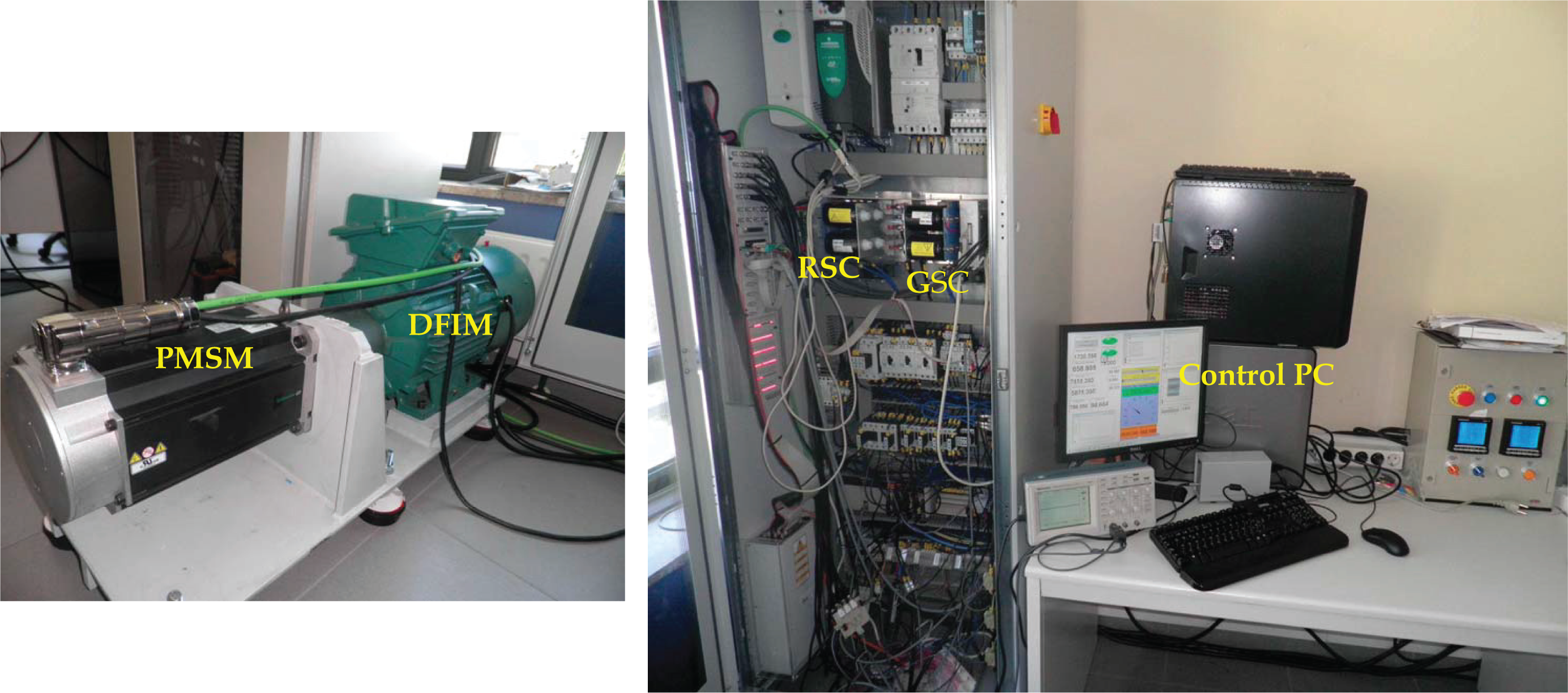
In this section the performance of the proposed adaptive sliding mode controller is analyzed. The experimental validation has been carried out in the experimental platform shown in Figure 3 that we have designed and constructed. The photography of this experimental platform is shown in Figure 4.

The control platform is formed by a PC with MatLab7/Simulink R2007a, dsControl 3.2.1 and the DS1103 Controller Board real time interface of dSpace, with a floating point PowerPC processor to 1 GHz. The electric machine used to implement the proposed controller is a commercial machine of Leroy Somer of 7.5 kW, 1447 rpm, double feed induction machine (

Table 1. Ratings and parameters of the DFIG (Leroy Somer).

Ratings and parameters	Values
Stator Voltage	380 V
Rotor Voltage	190 V
Rated stator current	18 A
Rated rotor current	24 A
Rated speed	1447 r.p.m.@ 50 Hz
Rated torque	50 Nm
Stator resistance	0.325 Ω
Rotor resistance	0.275 Ω
Magnetizing inductance	0.0664 H
Stator leakage inductance	0.00264 H
Rotor leakage inductance	0.00372 H
Inertia moment	0.07 Kg.m2

), connected to the grid through the rotor in a Back to Back configuration with two voltage source inverters. The wind profiles are generated by a 10.6 kW 190U2 Unimotor synchronous AC servo motor. The mechanical speed is measured using the servo motor incremental encoder of 4096 square impulses per revolution using the frequency measurement method. The rotor and stator currents are limited to the nominal values in order to protect the machine against over currents. All the sensors to measure the currents, voltages and speed are adapted and connected to the DS1103 Controller Board.

The DS1103 Controller Board controls both inverters generating the SVPWM (space vector pulse width modulation) pulses. The sample period is defined for the SVPWM frequency of 7 kHz, this is 143 μs. The dead time for the inverters used in this study is 1.5 μs and is controlled by software and hardware. The connection sequence of the DFIG to the grid begins with the charging of rotor and grid converters DC bus. Once this DC bus is charged and if the grid side reference system is oriented with the grid voltage the grid side converter is connected through contactor K1 and regulation of DC bus to a fixed value will begins.

Before realizing the connection of the stator to the grid, two steps have to be made first. The first one is the detection of the encoder offset respect the stator flux, and the second step is the synchronization of the stator voltage with the grid voltage. Once all the steps are finished, the stator will be connected to the grid trough contactor K2 and the regulation of active and reactive power will begin. The synchronization with the grid voltage is done by measuring the grid side voltage and using a PLL (Phase Locked Loop).

6.1. DFIG Simulation and Real Platform Validation

The simulation model of experimental platform has been implemented in Matlab/Simulink in order to test in advance the controllers in order to avoid undesirable damages in the experimental platform. When the controllers are proved in simulation then these controller are implemented in the experimental platform in order to show the real performance. The next experimental validation shows the correspondence between the simulation results using the simulation model implemented in Matlab/Simulink and the real experimental results using the experimental platform.

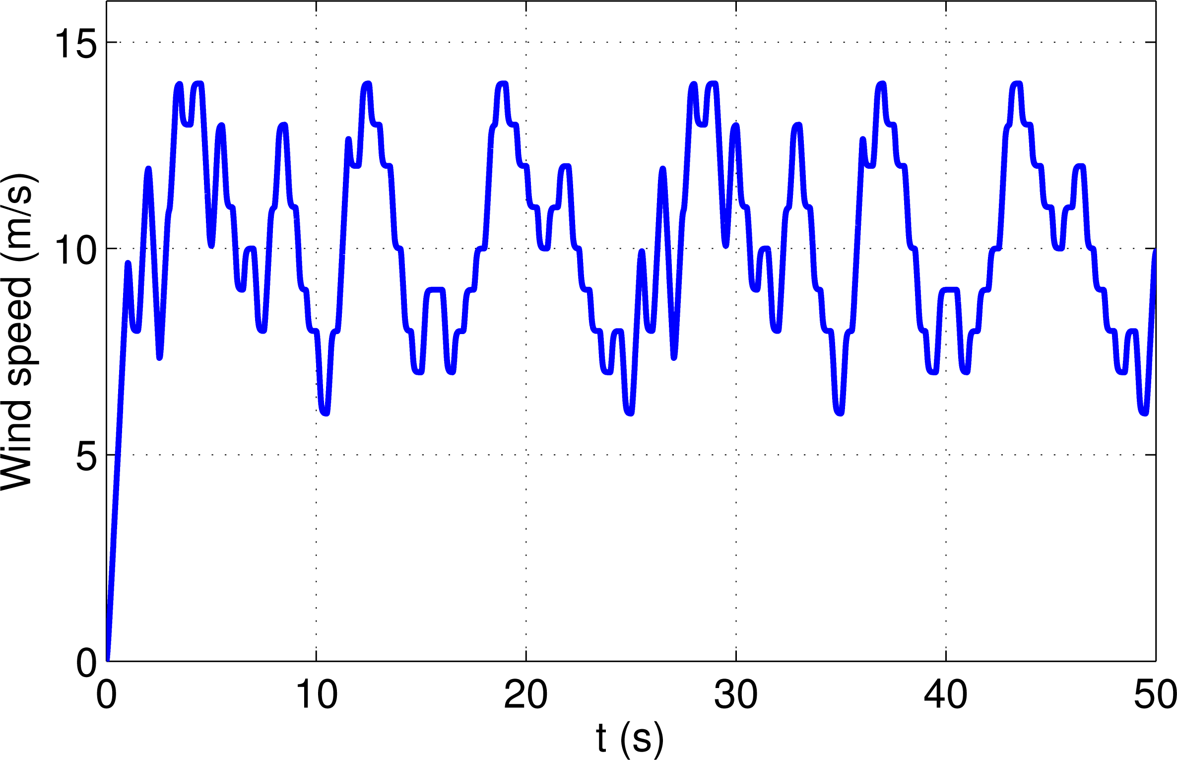
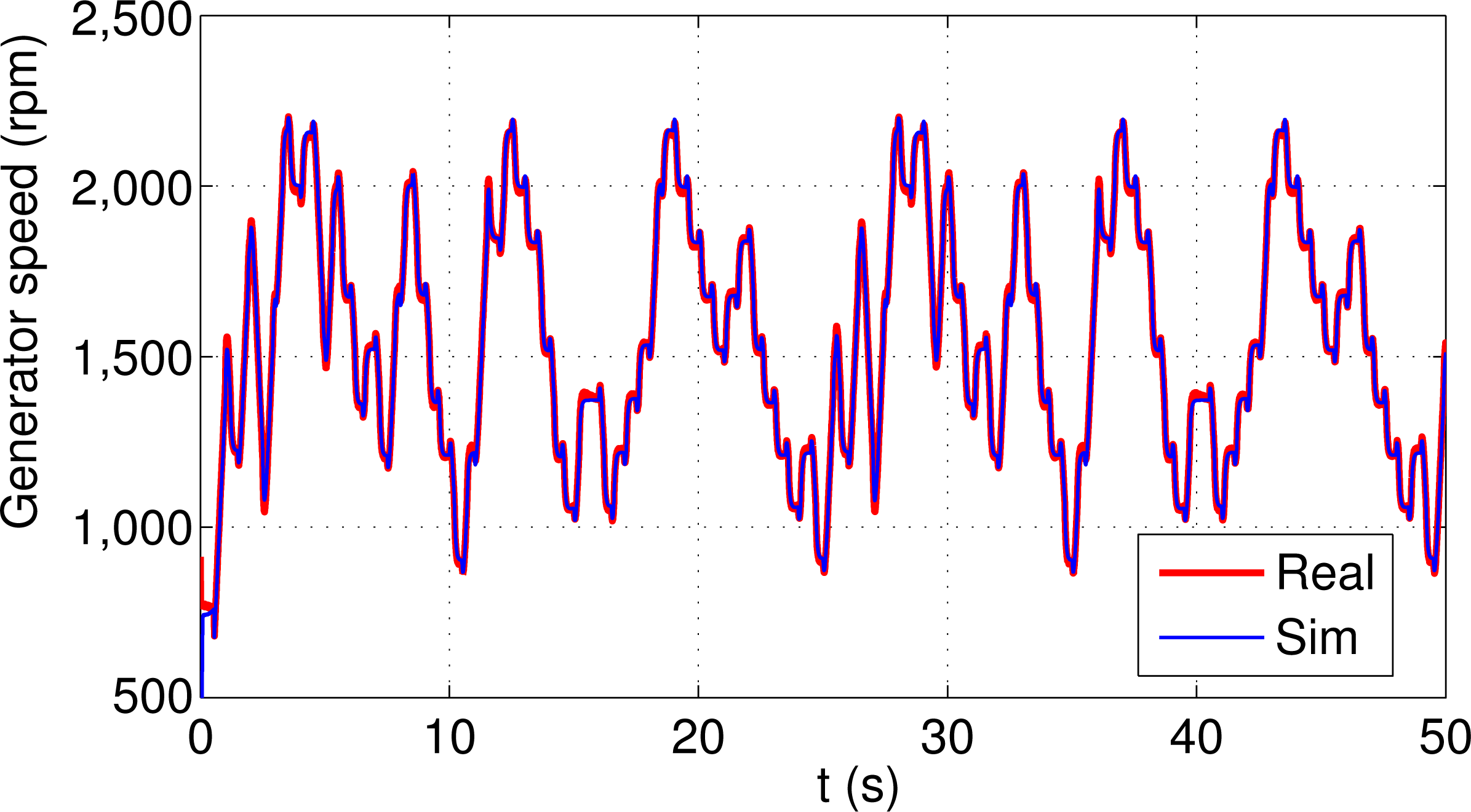
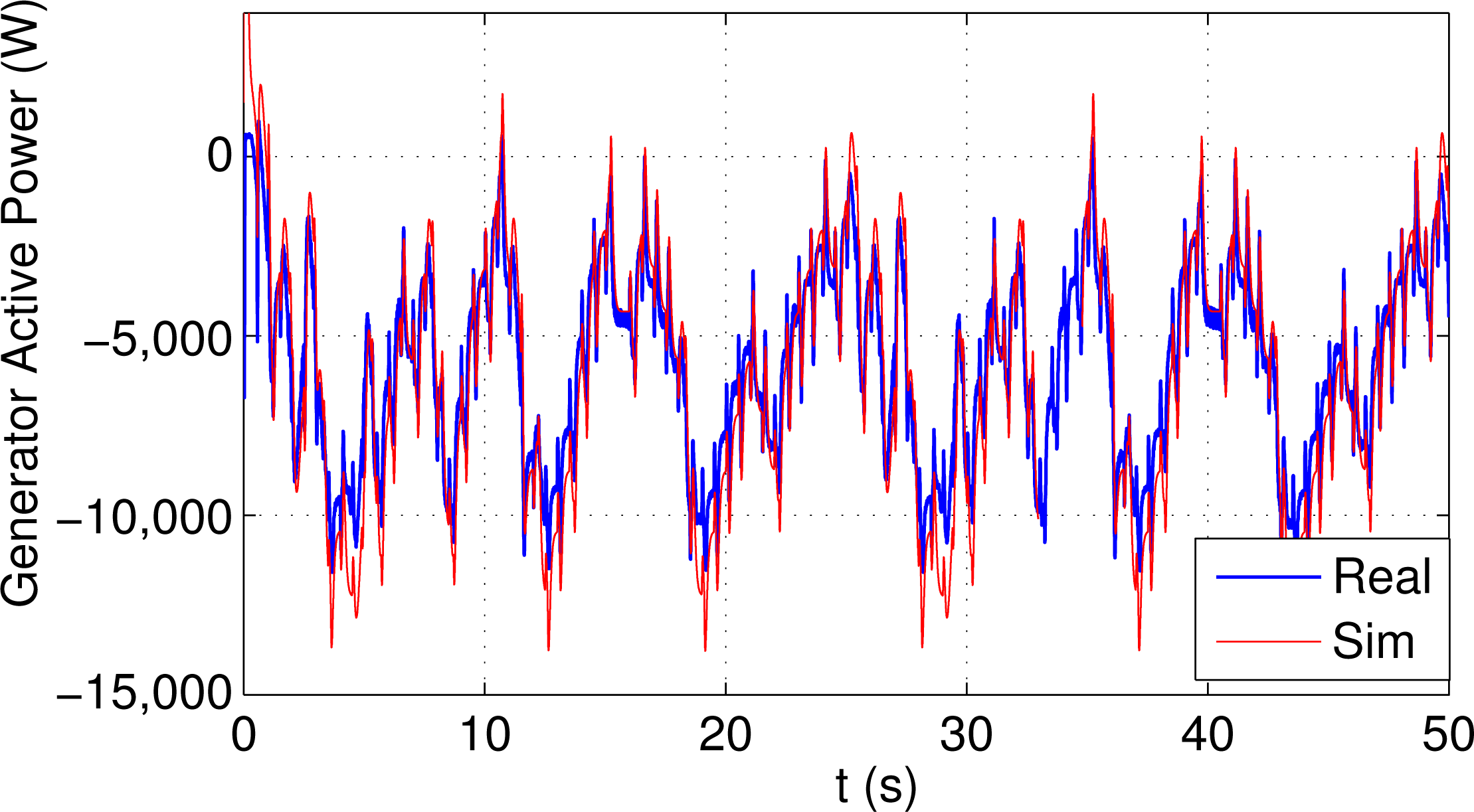
Figure 6 shows the real and simulated rotor speed using the same random wind profile show in Figure 5, and using a standard PID controller during 50 s. Figure 7 shows the real and simulated generator active power and Figure 8 shows the real and simulated rotor active power. As it can be observed, these figures shown a close behaviour between the simulation results obtained using the simulation model and the real results obtained in the experimental platform.

6.2. DFIG Speed Regulation to Get the Maximum Power Extraction

Now, the variable speed wind turbine regulation performance using the proposed sliding mode field oriented control scheme is tested in the presented test rig. The objective of this regulation is to maximize the wind power extraction in order to obtain the maximum electrical power from the wind. In this sense, the wind turbine speed must be adjusted continuously against the variations of wind speed. The DC bus voltage of the two inverters is regulated to 570 V using the proposed sliding-mode control scheme. The values for the rotor speed sliding mode controller are, β = 1, k = 0.5, a = 0.1, b = 1, and the values for the DC voltage sliding mode controller are, λ = 0.8, γ = 0.6.

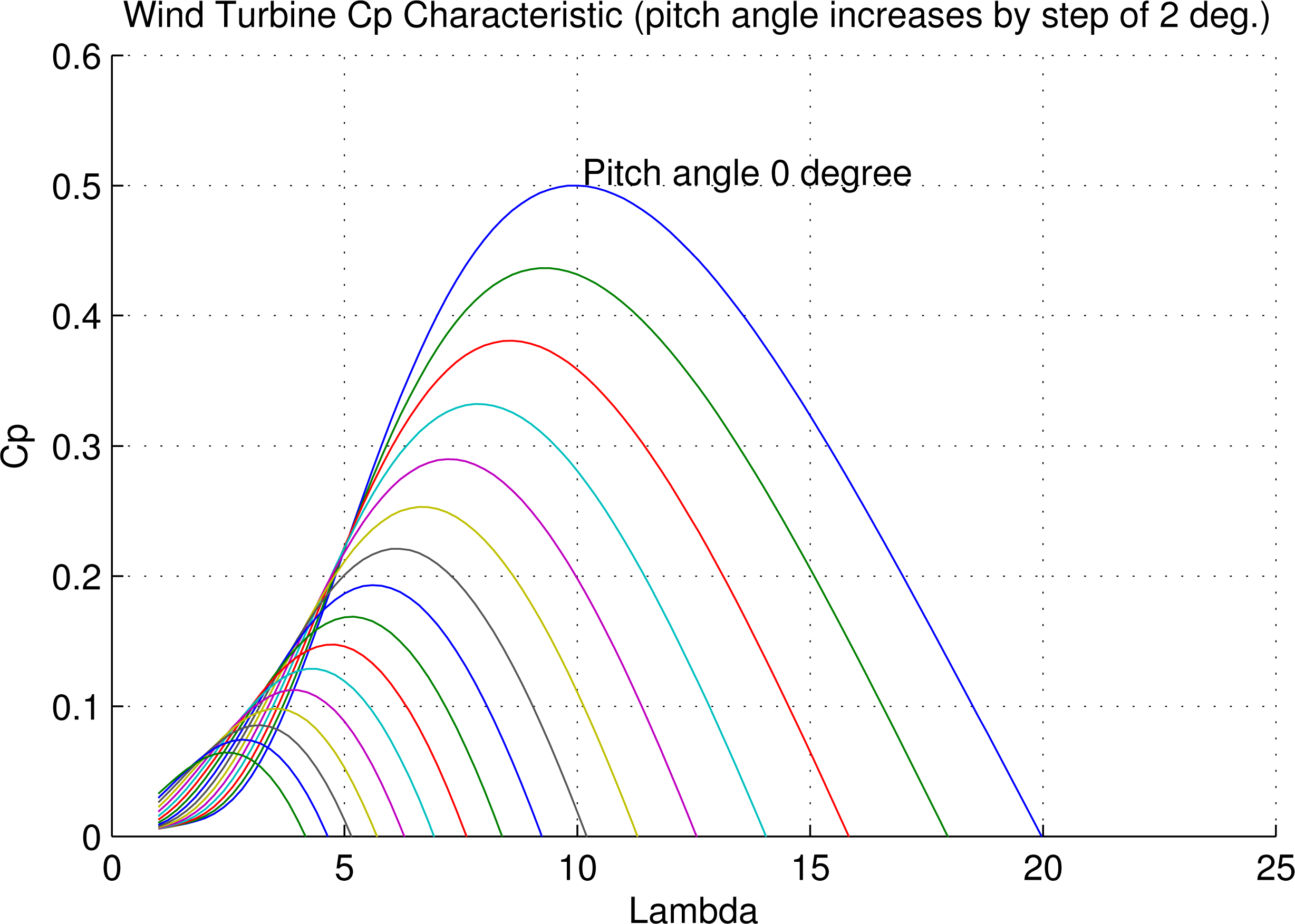
In the Figure 9, the power coefficient, C_p(λ, β), of the wind turbine, as a function of lambda, for different pitch angles, β, ranging from 0 to 30 degrees is displayed. This figure shows, that for β = 0, the lambda optimum value is λ_opt = 10, but for a larger pitch angle values the λ_opt value decreases.

In experimental test a variable wind speed input, show in the Figure 5, is used. As it can be seen in the figure, the wind speed varies between 6 m/s and 14 m/s, and therefore the proposed controller have to maximize the electric power production for a wide range of wind speeds.

Figure 10 shows the reference (Ref.) and the real rotor speed (Real). As it may be observed, after a transitory time, in which the sliding mode is reached, the rotor speed tracks the desired speed in spite of system uncertainties. Moreover, in this figure a good transient response can be observed because the system response do not presents overshoot nor oscillations.

Figure 11 shows the generated reactive power (Q) and the generated active power (P), whose value is maximized by our proposed sliding mode control scheme. The reactive reference is fixed to 0 VAR and the control shows that for strong changes of active power the reactive power is kept constant showing a good decoupling between both powers.

Figure 12 shows the rotor power. The power is positive (absorbed from the grid) when the rotor speed is lower than the synchronous speed. Instead, when the speed of the DFIG is higher than synchronous speed the power goes from the machine to the grid (negative power).

Figure 13 shows the DC link voltage response obtained using the proposed sliding mode control scheme. This figure shows that the proposed sliding mode control scheme maintains the DC-link voltage constant in spite of the system uncertainties and wind speed variations.

In the next example, the proposed SMC is compared with the traditional PID controller in order to shown the controller performance. In this experimental validation the step change in the wind speed shown in Figure 14 is used in order to show the controller performance under a sudden wind changes which is a difficult task for the controller. The values of the PI rotor speed controller for comparison purposes are K_p = 2, K_i = 1 and K_d = 0.1.

Figure 15 shows the rotor speed regulation performance using the proposed SMC and the traditional PID controller. In this figure it can be observed that using the SMC controller the rotor speed tracks the reference speed that provides the maximum power extraction from the wind. Obviously due to the system mechanical inertia, the rotor speed can not track the speed changes in the reference speed but after a 0.05 s the reference speed is reached. The figure also shown that the response rate of the PID controller is similar to the response rate of the SMC controller and both controllers provides a similar rise time. However in the PID controller an overshoot can be observed, and therefore the system takes more time to reach the reference speed that provides the maximum power extraction from this new wind speed value. This overshoot can be reduced increasing the derivative action of the controller but in this case a slower response will be obtained.

7. Conclusions

In this paper, a sliding mode vector control scheme for a doubly feed induction generator drive, used in variable speed wind power generation is described. A variable structure control is proposed, which has an integral sliding surface to avoid the second derivative of the error signal, that is usual in the conventional sliding mode control schemes. Due to the nature of the sliding control, this control scheme is robust under uncertainties that usually appear in the real systems. The proposed control method allows to control the wind turbine operating with the optimum power efficiency over a wide range of wind speed, and therefore maximizes the power extraction for variable wind speeds.

At wind speeds of less than the rated wind speed, the speed controller seeks to maximize the power according to the maximum of the power coefficient curve. As a result, the variation of the generator speed follows the slow variation in the wind speed.

The closed loop stability of the presented design has been proved through the Lyapunov stability theory.

Finally, by means of some experiments in a real test bench, it has been shown that the proposed control scheme performs reasonably well in practice, and that the speed tracking objective is achieved in order maintain the maximum power extraction under system uncertainties.

References

- World Wind Energy Association, Half-Year World Wind Energy Report 2013, WWEA Head Office, Bonn, Germany, 2013.
- Badihi, H.; Zhang, Y.; Hong, H. Fuzzy gain-scheduled active fault-tolerant control of a wind turbine. J. Frankl. Inst 2014, 350, 3677–3706. [Google Scholar]
- Mohammadi, J.; Afsharnia, S.; Vaez-Zadeh, S. Efficient fault-ride-through control strategy of DFIG-based wind turbines during the grid faultsOriginal. Energy Convers. Manag 2014, 78, 88–95. [Google Scholar]
- You, R.; Barahona, B.; Chai, J.; Cutululis, N.C. A novel wind turbine concept based on an electromagnetic coupler and the study of its fault ride-through capability. Energies 2013, 6, 6120–6136. [Google Scholar]
- Kesraoui, M.; Chaib, A.; Meziane, A.; Boulezaz, A. Using a DFIG based wind turbine for grid current harmonics filtering. Energy Convers. Manag 2014, 78, 968–975. [Google Scholar]
- Muyeen, S.M.; Hasanien, H.M.; Al-Durra, A. Transient stability enhancement of wind farms connected to a multi-machine power system by using an adaptive ANN-controlled SMES. Energy Convers. Manag 2014, 78, 412–420. [Google Scholar]
- Akel, F.; Ghennam, T.; Berkouk, E.M.; Laour, M. An improved sensorless decoupled power control scheme of grid connected variable speed wind turbine generator. Energy Convers. Manag 2014, 78, 584–594. [Google Scholar]
- Wang, Y.; Wu, Q.; Xu, H.; Guo, Q.; Sun, H. Fast coordinated control of DFIG wind turbine generators for low and high voltage ride-through. Energies 2014, 7, 4140–4156. [Google Scholar]
- Rodriguez, J.; Fernandez, A.; Hermoso, A.; Veganzones, N. Low voltage ride-through in DFIG wind generators by controlling the rotor current without crowbars. Energies 2014, 7, 498–519. [Google Scholar]
- Pande, V.N.; Mate, U.M.; Kurode, S. Discrete sliding mode control strategy for direct real and reactive power regulation of wind driven DFIG. Electr. Power Syst. Res 2013, 100, 73–81. [Google Scholar]
- Muller, S.; Deicke, M.; de Doncker, R.W. Doubly fed induction generator system for wind turbines. IEEE Ind. Appl. Mag 2002, 8, 26–33. [Google Scholar]
- Bravo, A.; Gomez-Gil, F.J.; Martin, J.V.; Ausin, J.; Ruiz, J.; Pelaez, J. Feasibility of a simple small wind turbine with variable-speed regulation made of commercial components. Energies 2013, 6, 3373–3391. [Google Scholar]
- Chen, J.-H.; Yau, H.-T.; Hung, W. Design and study on sliding mode extremum seeking control of the chaos embedded particle swarm optimization for maximum power point tracking in wind power systems. Energies 2014, 7, 1706–1720. [Google Scholar]
- Barambones, O. Sliding mode control strategy for wind turbine power maximization. Energies 2012, 5, 2310–2330. [Google Scholar]
- Vidal, Y.; Acho, L.; Luo, N.; Zapateiro, M.; Pozo, F. Power control design for variable-speed wind turbines. Energies 2012, 5, 3033–3050. [Google Scholar]
- Pena, R.; Clare, J.C.; Asher, G.M. Doubly fed induction generator using back-to-back PWM converters and its application to variablespeed wind-energy generation. Proc. Inst. Elect. Eng 1996, 143, 231–241. [Google Scholar]
- Lei, Y.Z.; Mullane, A.; Lightbody, G.; Yacamini, R. Modeling of the wind turbine with a doubly fed induction generator for grid integration studies. IEEE Trans. Energy Convers 2006, 21, 257–264. [Google Scholar]
- Joselin, G.M.; Iniyan, S.; Sreevalsan, E.; Rajapandian, S. A review of wind energy technologies. Renew. Sustain. Energy Rev 2007, 11, 1117–1145. [Google Scholar]
- Heier, S. Grid Integration of Wind Energy Conversion Systems; John Wiley & Sons Ltd: West Sussex, UK, 1998; ISBN: 0-471-97143-X. [Google Scholar]
- Qiao, W.; Zhou, W.; Aller, J.M.; Harley, R.G. Wind speed estimation based sensorless output maximization control for a wind turbine driving a DFIG. IEEE Trans. Power Electron 2008, 23, 1156–1169. [Google Scholar]
- Utkin, V.I. Sliding mode control design principles and applications to electric drives. IEEE Trans. Ind. Elect 1993, 40, 26–36. [Google Scholar]
- SimPowerSystems 5. Users Guide; The MathWorks, Inc: Natick, MA, USA, 2010.