Transient Thunderstorm Downbursts and Their Effects on Wind Turbines


Abstract
: The International Electrotechnical Commission (IEC) Standard 61400-1 for the design of wind turbines does not explicitly address site-specific conditions associated with anomalous atmospheric events or conditions. Examples of off-standard atmospheric conditions include thunderstorm downbursts, hurricanes, tornadoes, low-level jets, etc. The simulation of thunderstorm downbursts and associated loads on a utility-scale wind turbine is the focus of this study. Since the problem has not received sufficient attention, especially in terms of design, we thus focus in this paper on practical aspects. A wind field model that incorporates component non-turbulent and turbulent parts is described and employed in inflow simulations. The non-turbulent part is based on an available analytical model with some modifications, while the turbulent part is simulated as a stochastic process using standard turbulence power spectral density functions and coherence functions whose defining parameters are related to the downburst characteristics such as the storm translation velocity. Available information on recorded downbursts is used to define two storm scenarios that are studied. Rotor loads are generated using stochastic simulation of the aeroelastic response of a model of a utility-scale 5-MW turbine. An illustrative single storm simulation and the associated turbine response are used to discuss load characteristics and to highlight storm-related and environmental parameters of interest. Extensive simulations for two downbursts are then conducted while varying the storm’s location and track relative to the turbine. Results suggest that wind turbine yaw and pitch control systems clearly influence overall system response. Results also highlight the important effects of both the turbulence as well as the downburst mean wind profiles on turbine extreme loads.1. Introduction
A thunderstorm downburst is defined as a strong downdraft that includes an outflow of potentially damaging winds at or near the ground [1]. The 1978 Northern Illinois Meteorological Research on Downbursts (NIMROD) and the 1982 Joint Airport Weather Studies (JAWS) field projects [1,2] were conducted to investigate downbursts since they posed a great threat to aviation. Both programs used a network of Doppler radar systems to study the structure and life cycle of downbursts. Since then, several approaches have been developed to simulate downbursts. Additional field studies have provided an improved understanding of the time-varying characteristics of downburst transients [3,4].
Following the NIMROD and JAWS projects, atmospheric scientists and wind engineers attempted to simulate downbursts, both experimentally and numerically. As stated previously, the motivation initially arose out of a need for enhanced aviation safety during thunderstorm downbursts. From an atmospheric science perspective, numerical models employed to simulate downbursts fall into two main categories: sub-cloud models and cloud-resolving downburst models [5]. Sub-cloud models include consideration of some sort of forcing that generates negative buoyancy in a storm in the upper portion of the model domain in order to initiate the downburst [6–8]; cloud-resolving downburst models, on the other hand, involve simulation of the full life cycle of the downburst-producing storm [9–12].
From an engineering perspective, researchers have developed models for representing downbursts with a focus on the effect that downburst winds have on structures. In wind engineering applications, downbursts are typically simulated as impinging jets. Numerical models include that of Nicholls et al. [13], which involved a 2-D large-eddy simulation (LES) of downburst winds flowing around a building. Kim and Hangan [14] developed a 2-D model using the commercial computational fluid dynamics (CFD) software (FLUENT, ANSYS, Inc., Canonsburg, PA, USA) to investigate the macro-scale flow dynamics of an impinging jet and aid in describing downbursts. Sengupta et al. [15] performed numerical and physical simulations of thunderstorm downbursts and studied their effects on structures. Mason et al. [16] developed a dry 2-D non-hydrostatic model implemented within a CFD commercial code (ANSYS CFX11, ANSYS, Inc., Canonsburg, PA, USA). While some of these models are based on commercially available codes, often using 2-D LES for turbulence, Das et al. [17] attempted to develop a numerical code for 3-D LES of an impinging jet with application to downbursts.
Analytical models for impinging jets with specific application to downbursts have also been developed. Such models describe only the non-turbulent (mean) wind field in a downburst. They include models developed by Oseguera and Bowles [18], Vicroy [19], Abd-Elaal et al. [20], Wood et al. [21], McConville et al. [22], Holmes and Oliver [23], and Chay et al. [24]. Of these, the model of Chay et al. [24] is a modified version of the Oseguera-Bowles [18] and Vicroy [19] models, in turn based on velocity profiles from the Terminal Area Simulation System (TASS) model, which used a meteorological framework to study the physical and dynamical character of convective clouds and storms [25]. These models describe an axisymmetric stagnation point flow and satisfy the mass continuity equation. The models include boundary layer effects near the ground and closely match real-world measurements from the NIMROD and JAWS projects.
Actual downburst-related loading on structures has been studied for several years. Chay and Letchford [26,27] investigated the pressure on a cube in both stationary and moving downbursts. Using a deterministic–stochastic hybrid model of downbursts, Chen and Letchford [28,29] studied downburst loads on a cantilevered structure and on a building. Due to frequent failures of high-voltage electricity transmission towers, downburst wind loads on transmission lines are also of concern [23]. There have been several studies of wind loads on transmission line structures, including those of Oliver et al. [30], Li [31], Shehata et al. [32], and Chay et al. [33]. To date, there have been no systematic studies carried out on the effect of thunderstorm downbursts on wind turbines. The present study seeks to address exactly this problem.
As discussed by Nguyen et al. [34], Nguyen and Manuel [35], the non-turbulent portion of the velocity field in a downburst may be defined using available analytical models [18,19,24] with some modifications, while the turbulent field may be simulated using well-established frequency-domain approaches [36,37]. Such full 4-D wind fields (describing three orthogonal wind velocity components at discrete points in 3-D space and at discrete time instants) may then be employed in wind turbine aeroelastic response and turbine loads studies—possible, for instance, using aeroelastic codes such as the open-source software, FAST [38]. FAST is an aeroelastic computer-aided engineering tool for horizontal-axis wind turbines developed at the National Renewable Energy Laboratory (NREL). In the present study, aeroelastic simulation of the response of the baseline NREL 5-MW wind turbine model [39] is undertaken; this leads to simulated time series of various turbine loads, motions, etc. The storms and associated downburst characteristics selected are taken from the NIMROD (1978) and JAWS (1982) project observations. An illustrative single thunderstorm downburst and associated turbine response simulation is first described in some detail to highlight important characteristics of the flow fields and specific turbine response and performance characteristics (e.g., related to turbine control systems). Then, a study of the variability in downburst characteristics on the study turbine is carried out by investigating the influence of variation in storm track and location on turbine extreme loads.
2. Wind Field Model for Thunderstorm Downbursts
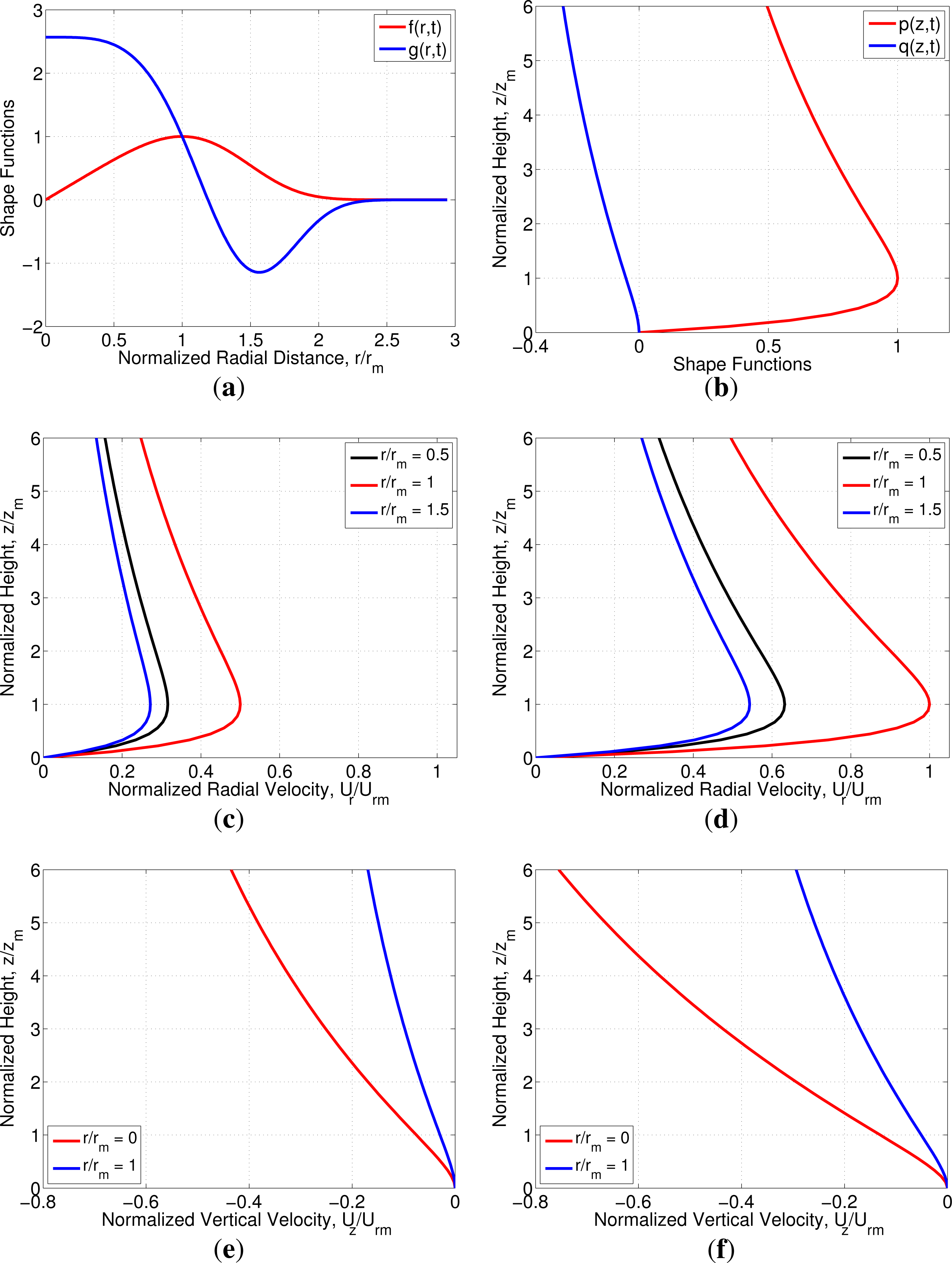
The wind field during thunderstorm downbursts may be represented by separately considering its non-turbulent (mean) and turbulent components. The non-turbulent wind velocity field is based on an analytical model [18,19,24] available in the literature. The radial velocity (Ur) and vertical velocity (Uz) components may be expressed as follows:
Figure 1 shows non-turbulent (mean) wind field shape functions indicating variation with radial distance and elevation as defined in Equations (3)–(6) as well as plots of the non-turbulent radial and vertical wind velocity profiles at different times, t = td/6 (when Π(t) = 0.5) and t = td/2 (when the storm is at its peak intensity, i.e., Π(t) = 1).
Note that a turbulent wind field is superimposed on the non-turbulent field in the turbine response simulations to be discussed. In general, downburst fluctuations are non-stationary in nature as has been confirmed from observations [3,4,40]; also, researchers [41–43] have proposed methods to generate non-stationary turbulence in thunderstorm downbursts. In this study, the turbulent component of the full downburst wind velocity field is modeled in a similar manner as is done for non-thunderstorm boundary layer flow fields, except that the turbulence intensity for each turbulence component scales with the storm’s translation speed; the turbulent wind field is simulated using the open-source turbulence simulator, TurbSim [37].
3. Problem Description and Assumptions
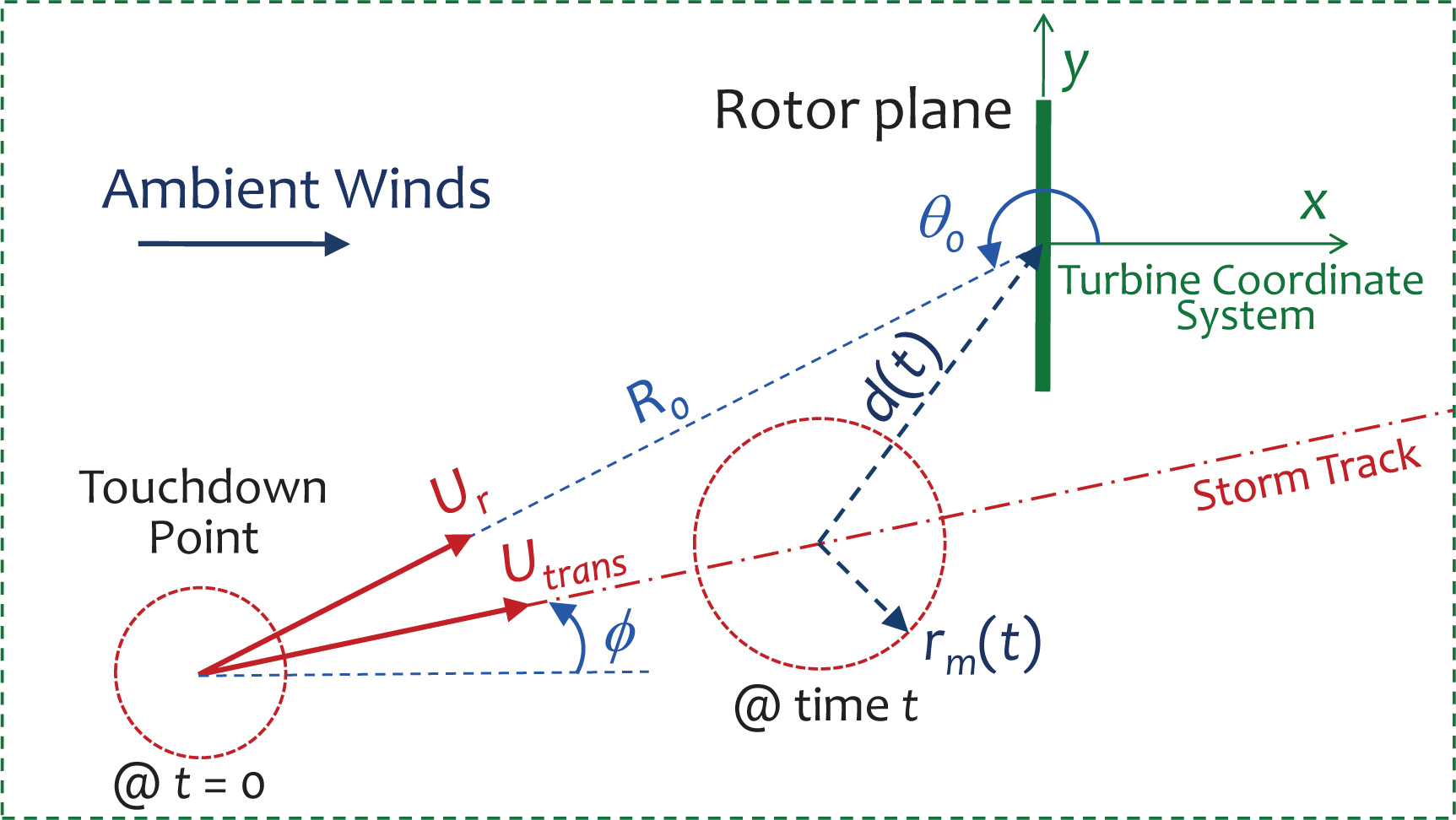
Figure 2 shows a plan view of a downburst scenario that depicts the wind turbine and a generalized storm touchdown and track. The storm touchdown point (i.e., its center at t = 0) is assumed to be defined by polar coordinates, (R0, θ0), relative to a coordinate system defined at the turbine. The storm is assumed to move in a straight line (its track) at a constant translation speed, Utrans. The angle, ϕ, which defines the direction of the storm translation relative to the ambient wind, Uamb, is assumed to be constant. The storm’s outflow is assumed to be influenced by the boundary layer environmental winds, Uamb(z) [2]; this ambient wind profile, Uamb(z) (directed along the x direction), is modeled by a power law with a shear exponent of 0.2 in this study. The wind velocity field that the turbine experiences at any time, t, during the downburst is related to the distance, d(t), from the storm center to the turbine at that time:
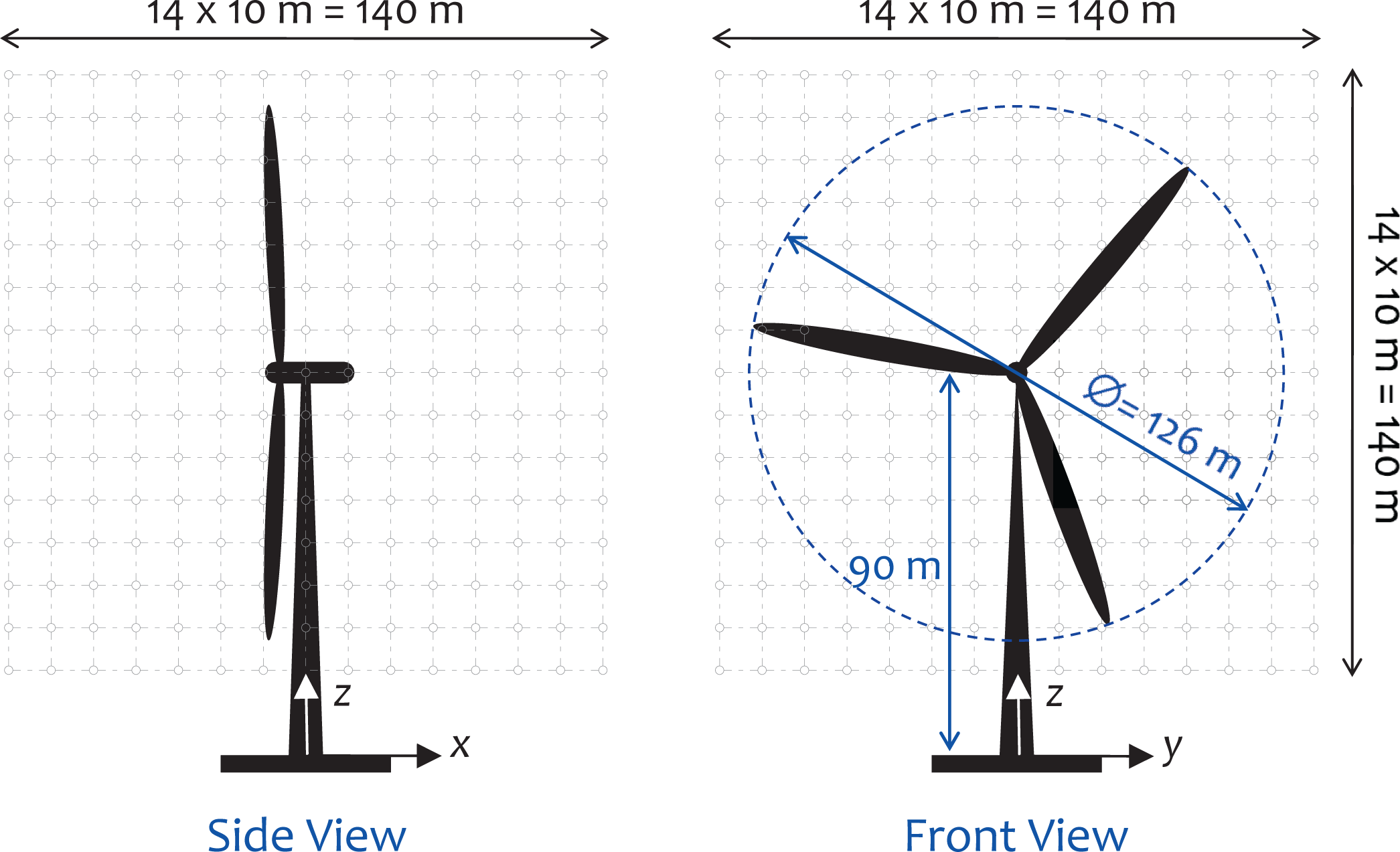
Table 1 provides a summary of the important properties and dimensions of the selected 5-MW wind turbine model for this study. Assumptions on turbine control and performance are made as follows: (i) When yaw control is required, the yaw rate is first set at the rate of the non-turbulent wind direction change as long as this rate of change in wind direction is small; if/when this rate of change in wind direction becomes significant, this yaw rate is set to a maximum of 0.3 degree/s. Up to 45 degree of yaw error/misalignment is allowed (i.e., the turbine is assumed to continue to operate as long as the yaw misalignment stays below 45 degree); (ii) Wind speeds above the turbine’s cut-out wind speed are permitted during the downburst; the pitch control logic for wind speeds above cut-out is assumed to be the same as that for wind speeds below cut-out. Figure 3 shows the pitch control, turbine rotor speed, power curve, and the steady-state flapwise bending moment at the root of a blade as a function of the wind speed at hub height (90 m AGL).
4. Numerical Studies
4.1. Definition of Downburst Cases
Two downbursts from the NIMROD and JAWS [1,2] projects are studied. For the selected downburst model, the required parameters and functions required for its complete description were estimated using the available information. Table 2 summarizes parameters/functions for the two downbursts (selected from the NIMROD and JAWS projects) that are simulated.
4.2. An Illustrative Turbine Response Simulation—Joint Airport Weather Studies “Average” Case
An illustrative single thunderstorm downburst and associated turbine response simulation is first discussed in some detail to highlight important characteristics of the flow fields and specific turbine response and performance characteristics (e.g., related to control systems). The JAWS “average” downburst is chosen for this purpose; its non-turbulent velocity field is computed using the model of Chay et al. [24] modified by the authors. The storm parameters needed for use with Equations (1) and (2) are given in Table 2. The storm touchdown point and direction of translation are chosen such that R0 = 4 km, θ0 = 180 degree, and ϕ = 15 degree (see Figure 2). Two values of the ambient wind speed at 90 m are considered—a base case of 6 m/s (below rated) as shown in Table 2 and another case of 12 m/s (above rated). For the non-turbulent wind velocity field simulations, a 140 m × 140 m × 140 m grid with 10 m spacing and centered at the turbine hub is employed (see Figure 4); each thunderstorm downburst simulation is run for 1000 s with a time step, Δt, equal to 0.05 s. As a result, wind velocity time series are generated at 153 = 3375 points on the grid described; each time series is comprised of 20,000 simulated wind velocity values. The turbulent portion of the wind velocity field during the thunderstorm downburst uses the Fourier-based Veers method [36,37] over a rectangular grid describing a vertical plane at x = 0; it uses the same temporal sampling and is simulated for the same duration as the non-turbulent field. The turbine response is simulated for two scenarios: with and without yaw control.
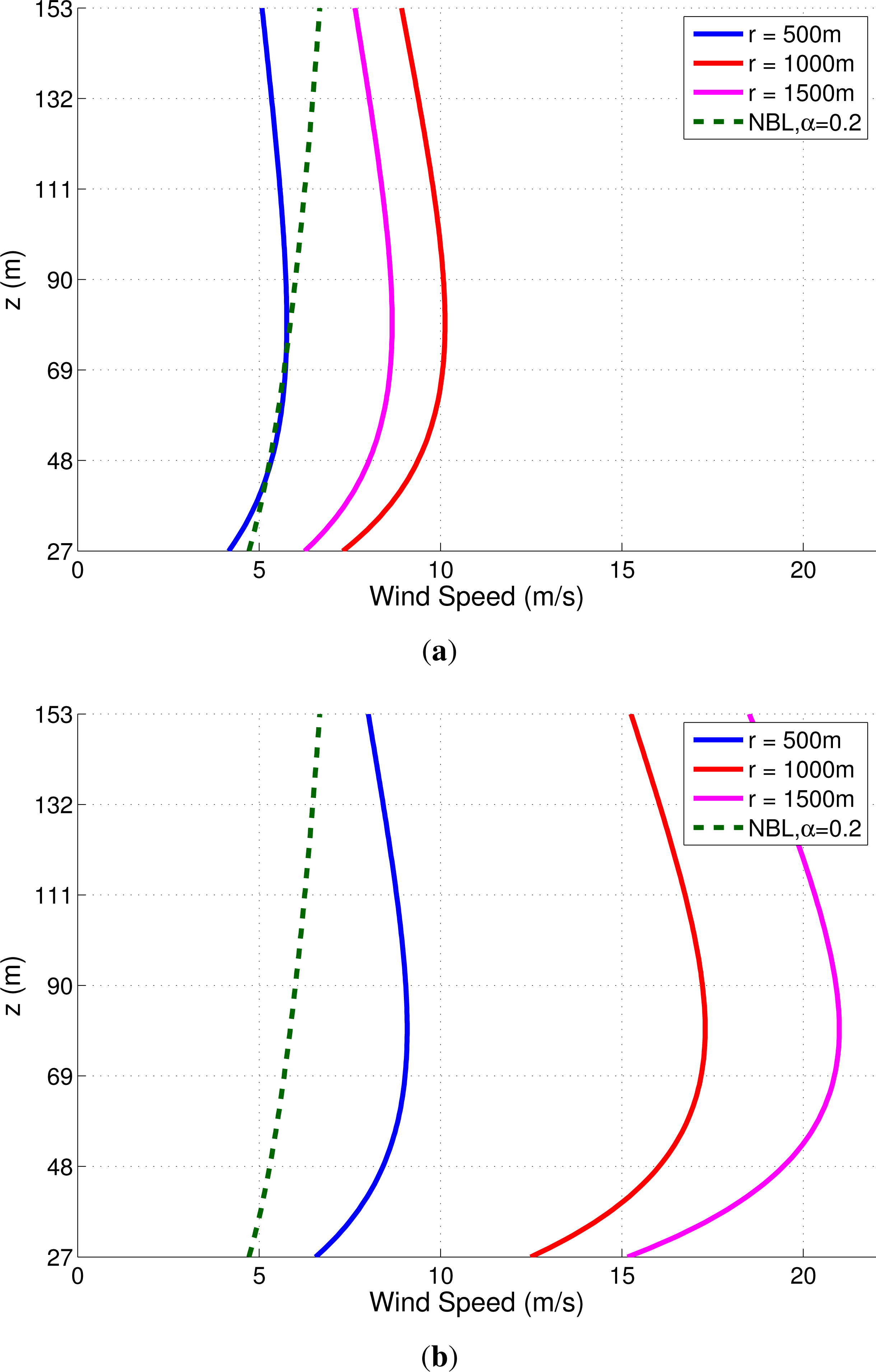
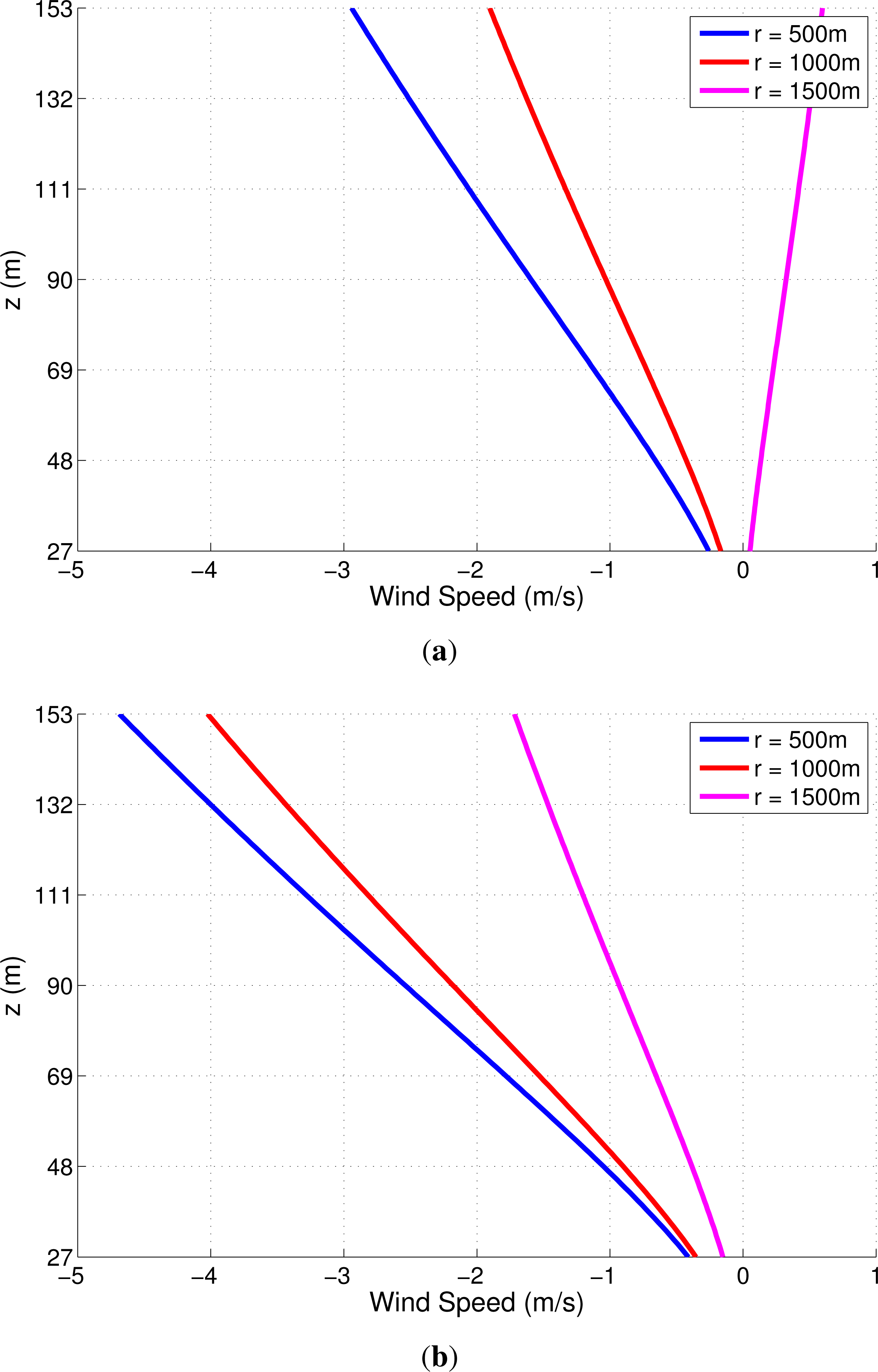
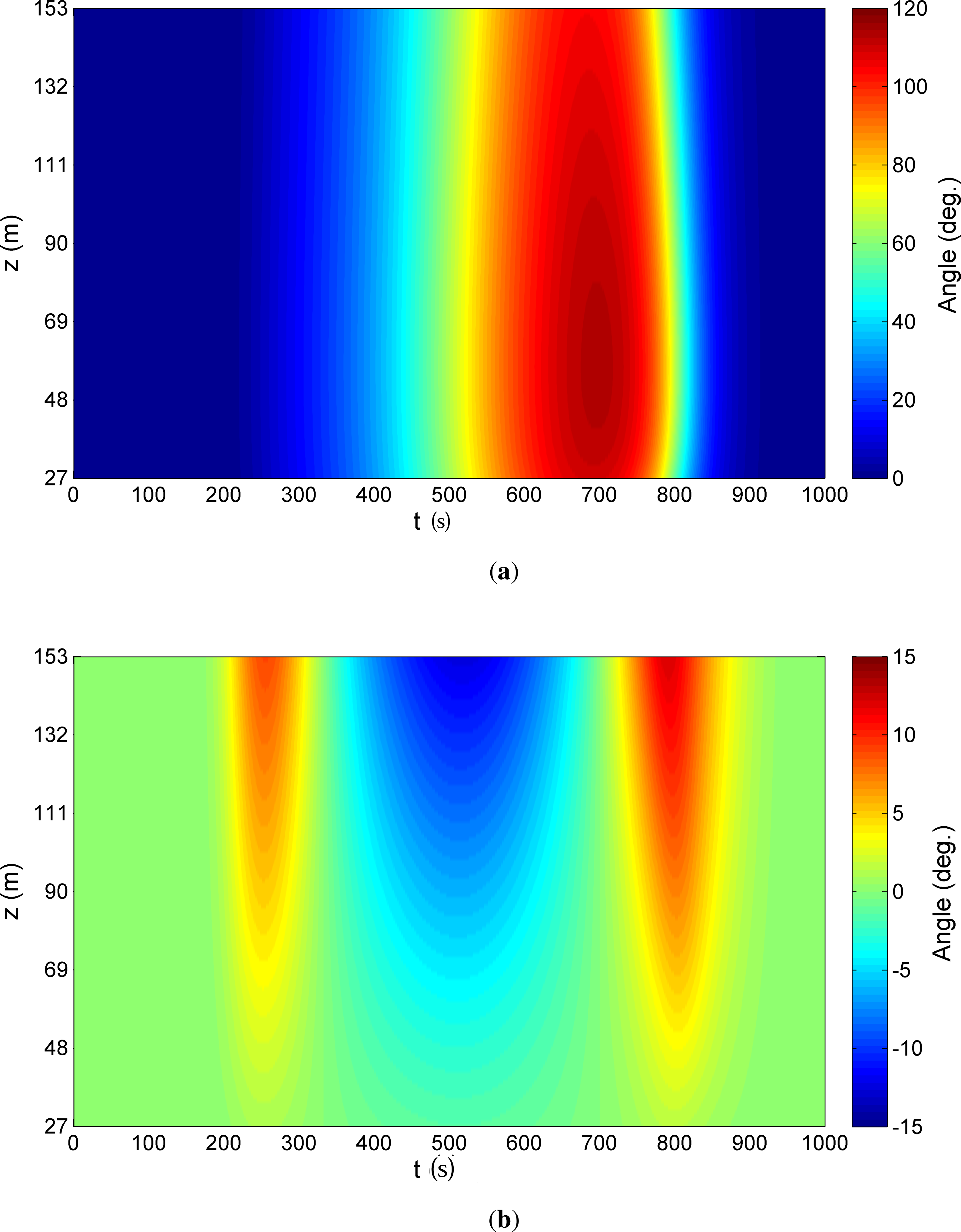
Although computations were carried out by including the turbulent component, for clarity in presentation, the following figures show time series that depict effects due to the non-turbulent wind field alone. Figures 5 and 6 show the variation with elevation of the horizontal (radial) and vertical wind shear, respectively, over the rotor (from z = 27 m to z = 153 m). The figures are presented for two time instants, t = td/6 and t = td/2, when the downburst intensity, Π(t) is 0.5 and 1.0, respectively; the figures depict profiles corresponding to radial distances from the downburst center equal to 500 m, 1000 m, and 1500 m. For the sake of comparison, dashed lines are included in Figure 5 that describe the neutral boundary layer (NBL) horizontal wind profile assuming a shear exponent of 0.2; downburst wind shear is significantly different from that in the neutral boundary layer. The non-turbulent horizontal and vertical veer profiles (or wind direction variation with elevation) during the downburst are presented in Figure 7; it is evident that wind directions not only vary significantly with time during the downburst but we notice that there can be some variation, at a fixed point in time, between the wind direction experienced by the lower and upper parts of the rotor.
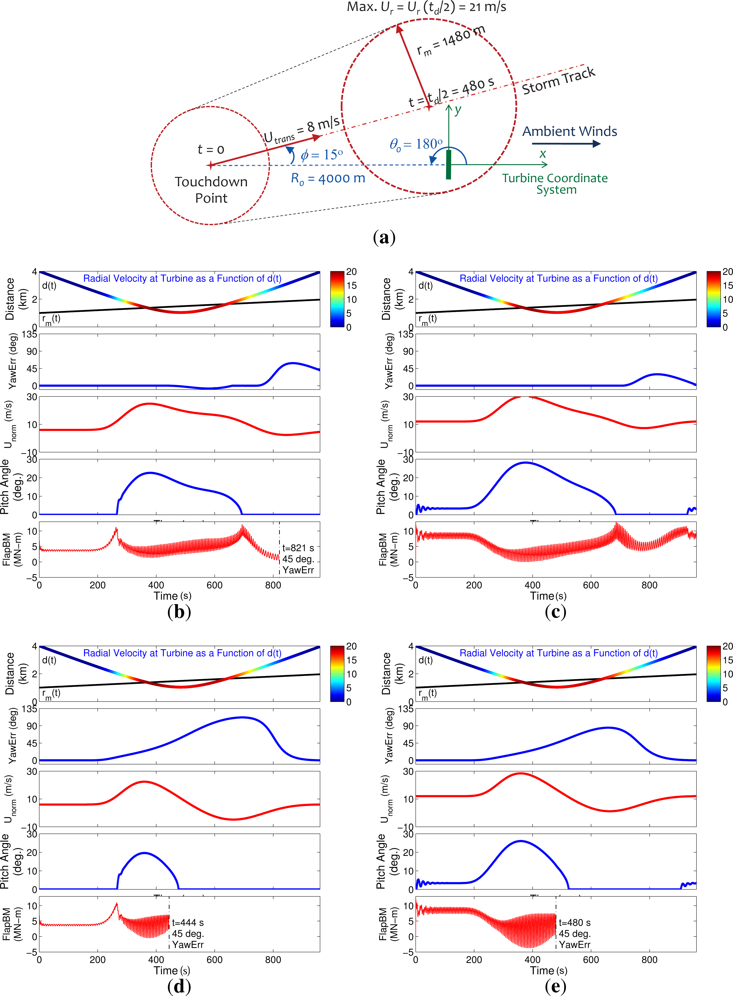
Figure 8a shows a plan view of the moving downburst and the turbine for the selected downburst simulation. The centers of the circles describe the downburst locations at the beginning of the event and after 8 min. Since the duration of the downburst, td, is 16 min, the storm is at its peak intensity at 8 min, when the maximum radial velocity is 21 m/s. Points on the circumference of these circles are where the maximum radial velocity occurs; note that the radius to maximum winds, rm(t), increases with time (at t = 8 min, the radius to the maximum wind is 1480 m). The storm touchdown point is initially 4 km from the turbine; in this simulation, the moving downburst is within 1.5 km of the turbine at t = 8 min, and the radial velocity experienced by the turbine then is less than 21 m/s.
4.2.1. Joint Airport Weather Studies “Average” Case: Uamb = 6 m/s; with Yaw Control
Figure 8b corresponds to the scenario where the ambient wind speed at 90 m is 6 m/s and yaw control is applied. The upper panel of the figure shows the variation with time of the distance, d(t), separating the center of the storm from the turbine; the radial distance from the storm center, rm(t), where the maximum velocity occurs; and the radial velocity at the turbine, shown with color variation, on the d(t) plot. The storm-to-turbine distance, d(t), indicates whether the storm is moving toward or away from the turbine. The radial distance to the maximum velocity is an indication of the changing size (i.e., spatial extent) of the storm. The plots of d(t) and rm(t), taken together, give an indication of the changing strength of the wind velocity that the turbine experiences through the storm. At points in time where plots of d(t) and rm(t) intersect, the turbine is experiencing the largest instantaneous winds—for instance, at t ≈ 350 s and, again, at t ≈ 640 s, the turbine is at points during the storm where radial velocities are largest. Note that these identified time instants are not when the storm is at its peak intensity.
The next panels in Figure 8b show the yaw misalignment angle time series; the simulated wind velocity normal to the rotor plane at hub height, Unorm; the time-varying blade pitch angle; and the variation with time of the flapwise bending moment at a blade root. Between t = 0 s and t = 200 s, i.e., before the storm’s intensity is felt at the turbine, the mean wind speed at hub height (z = 90 m) is approximately 6 m/s, which is below the rated wind speed (11.4 m/s) for this turbine. At these low winds, the blade pitch angle is zero and the power generated is less than the rated 5 MW level (see Figure 3a). As the storm picks up in intensity, the wind speed increases and the flapwise bending moment increases as well, while the blade pitch angle remains at zero until the rated wind speed is reached. At the rated wind speed, i.e., at t ≈ 260 s, a first peak (or kink) in the flapwise bending moment time series is seen. Since the winds are continuing to increase, the blade pitch angle must increase in order to maintain the rated power of 5 MW and to limit structural loads (see Figure 3a). Higher wind speeds would be expected to increase loads on the blades; however, the increase in blade pitch angle leads to an offsetting greater reduction in the blade loads and leads to a decreasing flapwise bending moment starting at t ≈ 260 s. It is the change in blade pitch angle from a zero value that produces the kink in the response time series. As the winds get stronger, the blade pitch angle continues to increase and the flapwise bending moment continues to decrease. As the winds begin to decrease after t = 480 s, the blade pitch angle decreases and the flapwise bending moment starts to pick up. At t ≈ 700 s, the blade pitch angle goes to zero while the winds keep decreasing; then, flapwise loads also begin to decrease (this explains the second peak or kink in the flapwise bending moment time series). From this discussion, one can see that pitch control clearly influences the turbine response; whenever the pitch angle increases from zero or decreases to zero, there is a noticeable abrupt change or kink in the response. Note that the applied yaw control is adequate until t = 821 s when the yaw error exceeds 45 degree and the simulation is stopped.
4.2.2. Joint Airport Weather Studies “Average” Case: Uamb = 12 m/s; with Yaw Control
Figure 8c presents the similar scenario as in Figure 8b except that the ambient mean wind speed at hub height (z = 90 m) is increased from 6 m/s to 12 m/s. Before t = 200 s, for a 12 m/s wind speed at hub height, the blade pitch angle is already at about 3.5 degree (since the hub-height wind speed of 12 m/s is above the rated wind speed of 11.4 m/s), while the power output is at the rated value of 5 MW. As the wind speed increases further during the downburst, the flapwise bending moment decreases since the blade pitch angle has to increase while it maintains the rated power output of 5 MW. As the winds begin to decrease after t = 360 s, the blade pitch angle decreases as well, and the flapwise bending moment starts to pick up. At t ≈ 680 s, the blade pitch angle goes to zero while the winds keep decreasing; then, flapwise loads also begin to decrease (which results in a peak or kink in the flapwise bending moment time series). Note that the wind speed normal to the rotor plane, i.e., Unorm, can drop below the rated wind speed of 11.4 m/s, even while the mean ambient (x-direction) wind speed at hub height is 12 m/s, either because the turbine orientation is not perpendicular to the ambient wind direction (due to yaw misalignment) or because the downburst winds cancel out the ambient winds which can occur when the instantaneous location of the downburst moves downwind of the turbine. Interestingly, this higher ambient wind speed case (12 m/s at hub height) leads to smaller yaw error compared to when the ambient wind speed was 6 m/s; hence, the applied yaw control is adequate throughout the simulated downburst. Also, there is only one kink in the flap load time series in this case where the ambient winds are above the turbine’s rated wind speed.
4.2.3. Joint Airport Weather Studies “Average” Case: Uamb = 6 m/s; without Yaw Control
Figure 8d presents a similar scenario as that in Figure 8b except that no yaw control is imposed. In the absence of yaw control, the turbine experiences strongly yawed flows. High wind speeds and large as well as rapid wind direction changes result in larger turbine load ranges in comparison with the case with yaw control presented in Figure 8b. Note that, in the plots presented, for the sake of clarity, turbulence is excluded in the simulation. When turbulence is included, even larger response ranges (greater differences between two scenarios—i.e., with and without yaw control) are found [34]. In the absence of yaw control, the yaw error exceeds 45 degree in a shorter time and the simulation is stopped at t = 444 s before the second response/load peak is reached (this would have occurred at t ≈ 470 s when the pitch angle would have dropped to zero). Note that in this case, yaw error with no yaw control is effectively the same as the wind direction plot with time. Note that the plots showing yaw error in the absence of yaw control (such as in Figure 8d,e discussed next) are effectively the same as depicting the changing wind direction with time during the downburst.
4.2.4. Joint Airport Weather Studies “Average” Case: Uamb = 12 m/s; without Yaw Control
For the larger ambient wind case (12 m/s), similar to the case discussed in Figure 8c when turbine yaw control is not available, larger load range levels result as depicted in Figure 8e. At very high winds, up to ≈ 30 m/s, which is above the cut-out wind speed, blade pitch angles get very large while the power output and rotor speed are at their rated values (5 MW and 12.1 rpm, respectively). With high winds and large yaw error, the outermost portions of each blade can see negative angles of attack and thus negative lift forces. It is these forces that can deflect the blade upwind, subsequently causing negative bending flapwise moment values as seen in Figure 8e. Also, with no imposed yaw control, the yaw error exceeds 45 degree around t = 480 s.
4.3. Uncertainty in Storm Touchdown Location and Translation Direction
Different storm touchdown locations and translation directions relative to a wind turbine will result in different wind fields and, hence, different response/load levels experienced by the turbine. We discuss now the variability of such loads that result from the use of randomly selected values of R0, θ0, and ϕ (see Figure 2) where (i) only those storm-specific R0 values are selected that can cause significant loads are considered; (ii) only storms that begin upwind of the turbine are considered (i.e., where θ0 varies between 90 and 270 degree); and (iii) only storms with tracks defined such that ϕ lies between −45 degree and +45 degree are considered. For the two storms defined by the parameters/functions in Table 2, 1000 turbine response simulations were carried out with random realizations of R0, θ0, and ϕ.
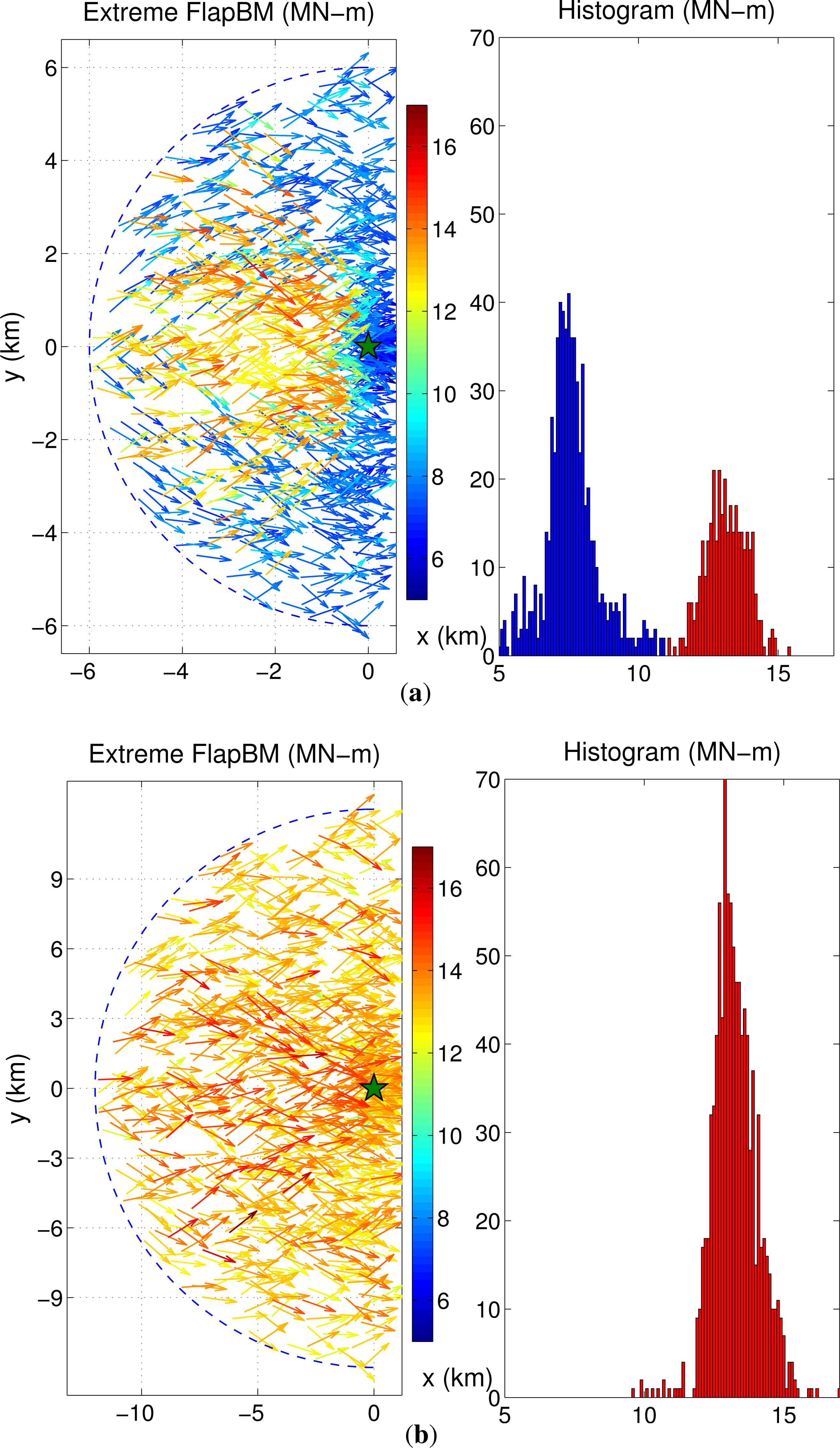
The plot in the left panel of Figure 9a shows the distribution of the extreme flapwise bending moment at a blade root resulting from 1000 simulations for the JAWS Average downburst; the root of each arrow indicates the touchdown location of the simulated downburst while the direction of each arrow indicates the translation direction of the storm in the associated turbine response simulation. The color of the arrows gives an indication of the magnitude of the corresponding peak load. Depending on the storm scenarios that result, the turbine may or may not experience the strongest intensity of the storm transient. If the storm does not quite reach the turbine or if the touchdown is close to the turbine but the storm is not fully developed then, low loads result (shown as blue arrows in the plot). These low loads make up the lower of the two modes in the histogram of extreme loads (shown in blue in the plot in the right panel of Figure 9a). Red arrows indicate cases where the downburst arrives at the turbine at close to its fully developed state; maximum loads are produced in these scenarios. These high loads lead to the higher of the two modes in the histogram of extreme load (shown in red in the plot in the right panel of Figure 9a). The plot in the left panel also reveals touchdown locations and associated translational direction that are critical to turbine loads. Note that the turbine is depicted by a green star at (x = 0, y = 0) on the plot. It appears that, in this particular case, a storm that hits the ground in a 90-degree sector centered symmetrically relative to the x-direction in the turbine’s upwind area and that moves toward to the turbine location causes large extreme loads.
The NIMROD Yorkville downburst, on the other hand, has quite different inflow characteristics, hence different load variability features (see Figure 9b). It has both a larger maximum radial velocity (31 m/s) as well as a faster translation speed (16 m/s). Furthermore, the ambient wind speed is 8 m/s at hub height (compared to 6 m/s for the JAWS Average downburst) which is closer to rated wind speed (11.4 m/s). According to the turbulence model used in this study, turbulence intensity scales with the storm’s translational speed. In ambient conditions with a (below-rated) wind speed of 8 m/s at hub height, the turbine response and loads are already fairly high. Strong turbulence during the storm, on its own, is expected to lead to large extreme loads. If, additionally, the storm approaches the turbine after touchdown, higher loads will arise also from the non-turbulent portion of the downburst’s wind field. In fact, peak turbine loads due to the strong turbulence (with mean wind speed close to rated) and those caused by the storm wind field are of almost the same order of magnitude; this is why a unimodal extreme load histogram (shown in the right panel of Figure 9b) results from the Yorkville downburst simulations. The plot in the left panel also confirms this unimodal load distribution as all the arrows share almost the same color everywhere.
Comparisons of the turbine response resulting from simulated thunderstorm downbursts from discrete events such as are defined for use with the Extreme Direction Change (EDC) and the Extreme Coherent Gust with Direction Change (ECD) load cases specified in the IEC 61400-1 standard were considered in a previous study by the authors [44]. Results showed that without yaw control, simulated downburst-related loads were found to be higher than those from both the EDC and ECD load cases. In the IEC 61400-1 design standard, there are design load cases (such as EDC and ECD as well as others) that were perhaps meant to capture the effect on flow fields (and, thus, on turbine loads) of transient events such as thunderstorm downbursts. On its own, the present study offers an alternative approach for modeling extreme thunderstorm-associated flow conditions, accompanied not only by high winds but also large and rapid wind direction changes.
4.4. Findings
Based on the example presented in Section 4.2, it is clear that large loads are not always associated with high winds. Excessive loads may result from fast-changing wind fields during which pitch and yaw controls may not respond sufficiently to limit loads. For example, rapidly changing winds from below-rated to above-rated levels, especially if accompanied by fast wind direction changes can lead to large loads. It is the storm translation speed and the storm duration that determine how fast a wind field will change. Fast-moving storms generally create unfavorable conditions for a wind turbine when both wind speed and wind direction can change rapidly. The ambient wind also has some effect on a turbine’s response during a downburst event; if the ambient wind (at hub height) is below the rated wind speed (11.4 m/s, for the 5 MW turbine), loads will likely get higher during the storm as was discussed in Section 4.2. If the ambient wind is already above the rated wind speed, loads will likely decrease during the storm as the winds increase, assuming available pitch/yaw control; this scenario was also discussed in a previous study [34]. While we have confined our load studies here to the blade root flapwise bending moment, in a more comprehensive study undertaken by Nguyen [45], the influence of downburst wind fields on tower-top yaw moments and on out-of-plane blade tip deflections was also studied and shown to be significant to about the same degree as that of the blade root flapwise bending moment.
5. Concluding Remarks
A wind field model for the simulation of thunderstorm downbursts was presented; non-turbulent and turbulent components of the field are generated separately. Two recorded downbursts, based on available information from field studies, were selected for a study of loads on a 5-MW wind turbine. During thunderstorm downbursts, high wind speeds and rapid direction changes can occur. Blade pitch control, established by changes to blade pitch angles, influences the rotor aerodynamics and can lead to a reduction in turbine loads during high winds that accompany downbursts. Yaw control limits yaw misalignment and can also reduce turbine loads especially in yawed flow conditions as when wind direction changes are rapid. An investigation of the influence of alternative storm scenarios on extreme loads for the 5-MW turbine was carried out by considering different storm touchdown locations and translation directions. Results indicate important influences on turbine extreme loads due to both ambient winds as well as downburst winds. For the storms studied, if the ambient winds are close to the turbine’s rated wind speed, extreme blade loads follow a unimodal distribution (strong turbulence also contributed when the large loads resulted due to ambient winds); if the ambient winds are lower than the rated speed, separate effects of the ambient winds and of the downburst winds lead to very different peak turbine loads and, hence, to markedly bimodal turbine extreme load distributions.
Acknowledgments
The authors are pleased to acknowledge the financial support received from Sandia National Laboratories by way of Contract No. 743358 and additional support from the National Science Foundation by way of Grant No. CBET-1336760.
Author Contributions
The first author prepared a draft of this manuscript and completed all the computations based on his Ph.D. dissertation. The second author made significant contributions to the initial written draft; he also served as Ph.D. supervisor and provided insights and guidance in all the computational work presented in this paper.
Conflicts of Interest
The authors declare no conflict of interest.
References
- Fujita, T. The Downburst: Microburst and Macroburst; University of Chicago: Chicago, IL, USA, 1985. [Google Scholar]
- Hjelmfelt, M. Structure and life cycle of microburst outflows observed in colorado. J. Appl. Meteorol 1988, 27, 900–927. [Google Scholar]
- Gast, K.D. A Comparison of Extreme Wind Events as Sampled in the 2002 Thunderstorm Outflow Experiment. Master’s Thesis, Texas Tech University, Lubbock, TX, USA. 2003. [Google Scholar]
- Orwig, K. Examining Strong Winds from a Time-Varying Perspective. Ph.D. Thesis, Texas Tech University, Lubbock, TX, USA. 2010. [Google Scholar]
- Orf, L.G.; Anderson, J.R. A numerical study of traveling microbursts. Mon. Weather Rev 1999, 127, 1244–1258. [Google Scholar]
- Anderson, J.R.; Orf, L.G.; Straka, J.M. A 3-D model system for simulating thunderstorm microburst outflows. Meteorol. Atmos. Phys 1992, 49, 125–131. [Google Scholar]
- Orf, L.G.; Anderson, J.R.; Straka, J.M. A three-dimensional numerical analysis of colliding microburst outflow dynamics. J. Atmos. Sci 1996, 53, 2490–2511. [Google Scholar]
- Anabor, V.; Rizza, U.; Nascimento, E.L.; Degrazia, G.A. Large-eddy simulation of a microburst. Atmos. Chem. Phys 2011, 11, 9323–9331. [Google Scholar]
- Hjelmfelt, M.R.; Roberts, R.D.; Orville, H.D.; Chen, J.P.; Kopp, F.J. Observational and numerical study of a microburst line-producing storm. J. Atmos. Sci 1989, 46, 2731–2744. [Google Scholar]
- Proctor, F.H. Numerical simulations of an isolated microburst, Part I: Dynamics and structure. J. Atmos. Sci 1988, 45, 3137–3160. [Google Scholar]
- Proctor, F.H. Numerical simulations of an isolated microburst, Part II: Sensitivity experiments. J. Atmos. Sci 1989, 46, 2143–2165. [Google Scholar]
- Straka, J.M.; Anderson, J.R. The Numerical simulations of microburst-producing thunderstorms: Some results from storms observed during the COHMEX experiment. J. Atmos. Sci 1993, 50, 1329–1348. [Google Scholar]
- Nicholls, M.; Pielke, R.; Meroney, R. Large eddy simulation of microburst winds flowing around a building. J. Wind Eng. Ind. Aerodyn 1993, 46, 229–237. [Google Scholar]
- Kim, J.; Hangan, H. Numerical simulations of impinging jets with application to downbursts. J. Wind Eng. Ind. Aerodyn 2007, 95, 279–298. [Google Scholar]
- Sengupta, A.; Sarkar, P.P.; Rajagopalan, G. Numerical and physical simulation of thunderstorm downdraft winds and their effects on buildings. Proceedings of the First American Conference on Wind Engineering, Clemson, SC, USA, 3–6 June 2001.
- Mason, M.S.; Wood, G.S.; Fletcher, D.F. Numerical simulation of downburst winds. J. Wind Eng. Ind. Aerodyn 2009, 97, 523–539. [Google Scholar]
- Das, K.K.; Ghosh, A.K.; Sinhamahapatra, K.P. Development of a numerical code for 3D LES simulation of thunderstorm downburst. In Proceedings of the Fifth International Symposium on Computational Wind Engineering (CWE2010), Chapel Hill, NC, USA, 23–27 May 2010.
- Oseguera, R.M.; Bowles, R.L. A Simple, Analytics 3-dimensional Downburst Model Based on Boundary Layer Stagnation Flow; Technical Report NASATM-100632; The National Aeronautics and Space Administration Langley Research Center: Hampton, VA, USA, 1988. [Google Scholar]
- Vicroy, D.D. A Simple, Analytical, Axisymmetric Microburst Model for Downdraft Estimation; Technical Report NASATM-100632; The National Aeronautics and Space Administration Langley Research Center: Hampton, VA, USA, 1988. [Google Scholar]
- Abd-Elaal, E.; Mills, J.; Ma, X. An analytical model for simulating steady-state flows of downburst. J. Wind Eng. Ind. Aerodyn 2013, 115, 53–64. [Google Scholar]
- Wood, G.S.; Kwok, K.C.S.; Motteramb, N.A.; Fletcherb, D.F. Physical and numerical modelling of thunderstorm downbursts. J. Wind Eng. Ind. Aerodyn 2001, 89, 535–552. [Google Scholar]
- McConville, A.; Sterling, M.; Baler, C. The physical simulation of thunderstorm downbursts using an impinging jet. Wind Struct 2002, 12-02, 133–149. [Google Scholar]
- Holmes, J.D.; Oliver, S.E. An empirical model of a downburst. Eng. Struct 2000, 22, 1167–1172. [Google Scholar]
- Chay, M.T.; Albermani, F.; Wilson, R. Numerical and analytical simulation of downburst wind loads. Eng. Struct 2006, 28, 240–254. [Google Scholar]
- Proctor, F.H. The Terminal Area Simulation System, Volume 1: Theoretical Formulation; NASA Contractor Report 4046, DOT/FAA/PM-85/50; The National Aeronautics and Space Administration, Scientific and Technical Information Branch: Hampton, VA, USA, 1987. [Google Scholar]
- Chay, M.T.; Letchford, C.W. Pressure distributions on a cube in a simulated thunderstorm downburst—Part A: Stationary downburst observations. J. Wind Eng. Ind. Aerodyn 2002, 90, 711–732. [Google Scholar]
- Chay, M.T.; Letchford, C.W. Pressure distributions on a cube in a simulated thunderstorm downburst—Part B: moving downburst observations. J. Wind Eng. Ind. Aerodyn 2002, 90, 733–753. [Google Scholar]
- Chen, L.; Letchford, C.W. A deterministic-stochastic hybrid model of downbursts and its impact on a cantilever structure. Eng. Struct 2004, 26, 619–645. [Google Scholar]
- Chen, L.; Letchford, C.W. Parametric study on the along-wind response of the CAARC building to downbursts in the time domain. J. Wind Eng. Ind. Aerodyn 2004, 92, 703–724. [Google Scholar]
- Oliver, S.E.; Moriarty, W.W.; Holmes, J.D. A Risk model for design of transmission line systems against thunderstorm downburst winds. Eng. Struct 2000, 22, 1173–1179. [Google Scholar]
- Li, C.Q. A stochastic model of severe thunderstorms for transmission line design. Probab. Eng. Mech 2000, 15, 359–364. [Google Scholar]
- Shehata, A.Y.; El Damatty, A.A.; Savory, E. Finite element modeling of transmission line under downburst wind loading. Finite Elem. Anal. Des 2005, 42, 71–89. [Google Scholar]
- Chay, M.T.; Albermani, F.G.; Hawes, H. Wind Loads on Transmission Line Structures in Simulated Downbursts. In Proceedings of the First World Congress on Asset Management, Gold Coast, Australia, 11–14 July 2006.
- Nguyen, H.; Manuel, L.; Veers, P. Simulation of Inflow Velocity Fields and Wind Turbine Loads during Thunderstorm Downbursts. In Proceedings of the 51st the Structural Dynamics and Materials Conference, Orlando, FL, USA, 12–15 April 2010.
- Nguyen, H.; Manuel, L. A Monte Carlo Simulation Study of Wind Turbine Loads in Thunderstorm Downbursts. In Proceedings of the 52nd Structural Dynamics and Materials Conference, Denver, CO, USA, 4–7 April 2011.
- Veers, P. Three-Dimensional Wind Simulation; Technical Report SAND88-0152; Sandia National Laboratory: Albuquerque, NM, USA, 1988. [Google Scholar]
- Jonkman, B. TurbSim User’s Guide: Version 1.50; Technical Report NREL/TP-500-46198; National Renewable Energy Laboratory: Golden, CO, USA, 2009. [Google Scholar]
- Jonkman, J.; Buhl, M. FAST User’s Guide, Technical Report NREL/EL-500-38230. National Renewable Energy Laboratory, Golden, CO, USA, 2005.
- Jonkman, J.; Butterfield, S.; Musial, W.; Scott, G. Definition ofa5MW Reference Wind Turbine for Offshore System Development, Technical Report NREL/TP-500-38060. National Renewable Energy Laboratory, Golden, CO, USA, 2009.
- Orwig, K.; Schroeder, J. Near-surface wind characteristics of extreme thunderstorm outflows. J. Wind Eng. Ind. Aerodyn 2007, 95, 565–584. [Google Scholar]
- Chen, L.; Letchford, C. Numerical simulation of extreme winds from thunderstorm downbursts. J. Wind Eng. Ind. Aerodyn 2007, 95, 977–990. [Google Scholar]
- Wang, L.; Kareem, A. Modeling of Non-stationary Winds in Gust Fronts. In Proceedings of the Ninth Joint Specialty Conference on Probabilistic Mechanics and Structural Reliability, Albuquerque, NM, USA, 26–28 July 2004.
- Kareem, A.; Kijewski, T. Time-frequency analysis of wind effects on structures. J. Wind Eng. Ind. Aerodyn 2002, 90, 1435–1452. [Google Scholar]
- Nguyen, H.H.; Manuel, L.; Veers, P. Wind turbine loads during simulated thunderstorm microbursts. J. Renew. Sustain. Energy 2011. [Google Scholar] [CrossRef]
- Nguyen, H.H. The Influence of Thunderstorm Downbursts on Wind Turbine Design. Ph.D. Thesis, The University of Texas at Austin, Austin, TX, USA. 2012. [Google Scholar]


| Properties/Dimensions | Values |
|---|---|
| Power rating | 5 MW |
| Rotor type | Upwind/three blades |
| Rotor diameter | 126 m |
| Hub height | 90 m |
| Cut-in, rated, cut-out | 3, 11.4, 25 m/s |
| Rated rotor speeds | 12.1 rpm |
| Rotor mass | 110,000 kg |
| Nacelle mass | 240,000 kg |
| Tower mass | 347,460 kg |
| Storm parameters | NIMROD Yorkville | JAWS average | |
|---|---|---|---|
| Urm | (m/s) | 31 | 21 |
| zm0 | (m) | 130 | 80 |
| kzm | (m/s) | 0.1 | 0.0 |
| rm0 | (m) | 940 | 1000 |
| krm | (m/s) | 0.5 | 1.0 |
| td | (min) | 20 | 16 |
| Utrans | (m/s) | 16 | 8 |
| Uamb at z = 90 m | (m/s) | 8 | 6 |
© 2014 by the authors; licensee MDPI, Basel, Switzerland This article is an open access article distributed under the terms and conditions of the Creative Commons Attribution license (http://creativecommons.org/licenses/by/3.0/).
Share and Cite
Nguyen, H.H.; Manuel, L. Transient Thunderstorm Downbursts and Their Effects on Wind Turbines. Energies 2014, 7, 6527-6548. https://doi.org/10.3390/en7106527
Nguyen HH, Manuel L. Transient Thunderstorm Downbursts and Their Effects on Wind Turbines. Energies. 2014; 7(10):6527-6548. https://doi.org/10.3390/en7106527
Chicago/Turabian StyleNguyen, Hieu H., and Lance Manuel. 2014. "Transient Thunderstorm Downbursts and Their Effects on Wind Turbines" Energies 7, no. 10: 6527-6548. https://doi.org/10.3390/en7106527