Modeling and Control of a Parallel Waste Heat Recovery System for Euro-VI Heavy-Duty Diesel Engines

Abstract

This paper presents the modeling and control of a waste heat recovery system for a Euro-VI heavy-duty truck engine. The considered waste heat recovery system consists of two parallel evaporators with expander and pumps mechanically coupled to the engine crankshaft. Compared to previous work, the waste heat recovery system modeling is improved by including evaporator models that combine the finite difference modeling approach with a moving boundary one. Over a specific cycle, the steady-state and dynamic temperature prediction accuracy improved on average by 2% and 7%. From a control design perspective, the objective is to maximize the waste heat recovery system output power. However, for safe system operation, the vapor state needs to be maintained before the expander under highly dynamic engine disturbances. To achieve this, a switching model predictive control strategy is developed. The proposed control strategy performance is demonstrated using the high-fidelity waste heat recovery system model subject to measured disturbances from an Euro-VI heavy-duty diesel engine. Simulations are performed using a cold-start World Harmonized Transient cycle that covers typical urban, rural and highway driving conditions. The model predictive control strategy provides 15% more time in vapor and recovered thermal energy than a classical proportional-integral (PI) control strategy. In the case that the model is accurately known, the proposed control strategy performance can be improved by 10% in terms of time in vapor and recovered thermal energy. This is demonstrated with an offline nonlinear model predictive control strategy.

1. Introduction

Nowadays, the primary power source for transportation is provided by internal combustion engines. Despite efforts to improve fuel economy in modern engines, approximately 60%–70% of the fuel power is still lost through the coolant and exhaust [1]. Moreover, the upcoming CO₂ emission legislation needs to be fulfilled. For heavy-duty vehicles, USA legislation indicates a 20% CO₂ emissions reduction by 2020. In Europe, similar requirements are expected to be introduced. To meet these upcoming CO₂ regulations and further reduce fuel consumption, diesel engines equipped with waste heat recovery (WHR) systems based on an organic Rankine cycle (ORC) seem very promising [2–4], especially for long-haul heavy-duty truck applications [5,6]. A WHR system allows energy to be recovered from the exhaust gas to generate mechanical power useful for propulsion.

For automotive applications, control of WHR systems is challenging. This is due to highly dynamic engine conditions, to interaction between the engine and the WHR system and to constraints, namely actuator limitations and safe operation. The control strategies dedicated to automotive applications are mostly based on a proportional-integral-derivative (PID) control type of approach [7–12]. However, this approach is most well established for single-input single-output systems. For multiple-input multiple-output systems with constraints, a model predictive control (MPC) can be developed, which, to the authors knowledge, has not been used for automotive WHR applications. Predictive control has been applied only to power plants [13,14] and refrigeration systems [15]. The main difference is that power plants and refrigeration systems work at different time scales as compared to automotive WHR systems that are governed by highly dynamic engine behavior.

In this paper, a switching model predictive control strategy is presented that considers the effect of highly dynamic engine disturbances caused by real on-road driving conditions. The WHR system is highly non-linear, mainly due to the two-phase flow phenomena. Thus, a global controller can give limited performance over the complete engine operating area. To account for this, a switching mechanism is developed that assigns a controller for a certain engine operating area. As a result, the control strategy allows operation close to the safety limit with good disturbance rejection properties. To benchmark the MPC strategy performance, a classical proportional-integral (PI) control strategy [16] is used, for comparison. Furthermore, an offline nonlinear MPC (NMPC) strategy is implemented to compare the MPC solution with the optimum solution in the case that the WHR system model is exactly known. The NMPC scheme is developed only for comparison purposes, since it is characterized by high computational complexity, making it unsuitable for embedded applications using off-the-shelf hardware.

For control design and optimization, dynamical modeling of WHR systems plays an important role. In [17], a dynamical model of the complete WHR system has been developed. The model captures the two-phase flow phenomena based on the conservation principles of mass and energy. However, in [17], simple evaporator models were used with simplified heat transfer coefficients. To improve the accuracy of the WHR system model, more advanced evaporator models are included, based on the approach used in [18] for the exhaust gas recirculation (EGR) evaporator. This approach combines the finite difference modeling approach with a moving boundary one. Thus, it is able to capture multiple phase transitions along a single pipe flow.

The paper is organized as follows. In Section 2, the experimental set-up is described. In Section 3, the improved WHR system model is presented and validated against the measurements. In Section 4, the control design and switching mechanism are presented. The control performance is evaluated in Section 5 by means of simulation results and comparison with a classical proportional-integral (PI) and NMPC control strategy. Conclusions and directions for future research are discussed in Section 6.

2. Experimental Set-Up

The experimental set-up is schematically illustrated in Figure 1. A six-cylinder Euro-VI European emission standards heavy-duty diesel engine is studied with an aftertreatment system that consists of: a diesel oxidation catalyst (DOC), diesel particulate filter (DPF), selective catalytic reduction (SCR) and an ammonia oxidation catalyst (AMOX). The engine is furthermore equipped with a WHR system that recovers heat from both the EGR line and main exhaust (EXH) line. The studied WHR system is based on a typical organic Rankine cycle (ORC) with pure ethanol as the working fluid. Ethanol is selected because of its physical and thermodynamic properties, which are suitable for this low temperature application. The ethanol is pumped from a reservoir at atmospheric pressure through plate-fin counter-flow evaporators, where it changes its state from liquid to two-phase and then vapor at the evaporator outlet. By expanding the vaporized ethanol, mechanical power is generated at the expander shaft. In this set-up, a two-piston expander is used that, according to the manufacturer data, can withstand ethanol in the two-phase state for short periods of time. To close the cycle, a condenser is used that brings the ethanol back to the liquid state. For safety reasons, a pressure relief valve is used that limits the system pressure to 60 bar.

The measurement system consists of thermocouples to measure temperature and thin-film pressure sensors. The exhaust gas mass flow rate is measured using Coriolis flow meters, while the ethanol mass flow rate is measured using helicoidal flow meters. To test the system under various engine loads and rotational speeds, a dynamometer is connected to the engine. To minimize heat losses to the environment, the WHR system was insulated.

Note that in the studied system, the expander and the pumps are mechanically coupled to the engine crankshaft. A disadvantage of this design is that due to mechanical coupling, the pressure in the system can be restricted, and thus, the power of the WHR system becomes limited. The advantage is that the mechanical power is directly transmitted to the engine, without energy losses from a power converter or variable transmission. During gear shifting, when the requested power is less than the WHR system net output power, P_req < P_whr, a throttle valve is closed (u_t = 0%) to avoid unwanted torque response. However, in this study, we focus only on the power mode (excluding gear shifting), and thus, the throttle valve is kept fully opened (u_t = 100%).

To avoid droplets, i.e., to guarantee the vapor state after the EGR evaporator and EXH evaporator, two bypass valves, u_egr and u_exh, are used. These bypass valves manipulate the ethanol flow rate, such that the vapor state is maintained after the evaporators in the presence of engine disturbances. On the exhaust gas side, the EGR valve u_g1 is controlled using the standard calibration for a conventional engine. From the cooling perspective, a valve u_g2 is used to bypass the exhaust gases at the EXH evaporator and, so, accommodates the maximum condenser cooling capacity.

3. Waste Heat Recovery System Modeling

The WHR system model is described using a component-based approach using first principle modeling. It consists of a reservoir, pumps, valves, evaporators, condenser and an expander model. The pumps and expander are map-based components, while the rest is modeled based on the conservation principles for mass and energy. The pipes, on the vapor side (indicated with red in Figure 1) are modeled as a compressible volume. The WHR system model is developed based on the following assumptions:

• the working fluid flows always in the positive direction;

• transport delays and pressure drops along the pipes are neglected;

• pressure drops along the evaporators are neglected on both the working fluid and exhaust gas side;

• the exhaust gas change in density along the evaporators is neglected;

• the condenser is ideal, so that the reservoir provides working fluid at the ambient pressure of 1 bar and a temperature of 65 °C.

Here, a brief review is given for the main components within the system, and more details can be found in [17,18].

3.1. Pump

The WHR system is equipped with two identical pumps. The mass flow rate through a pump is computed based on the ideal mass flow rate and volumetric efficiency as:

$${\dot{m}}_{\text{p}}={\dot{m}}_{\text{p},\text{id}}{\eta }_{\text{vol}}$$

(1)

where the volumetric efficiency η_vol = f(ω_p, p_r) is a function of pump speed ω_p (rev/s) and the pressure ratio across the pump p_r, according to the measurements. The ideal mass flow rate is given by:

$${\dot{m}}_{\text{p},\text{id}}=V_{\text{d}}{\omega }_{\text{p}}\rho$$

(2)

where V_d is the pump displacement volume and ρ is the working fluid density. The pump power is obtained using:

$$P_{\text{p}}={\dot{m}}_{\text{p}}\frac{p_{\text{out}}-p_{\text{in}}}{\rho {\eta }_{\text{is}}{\eta }_{\text{vol}}}$$

(3)

where η_is is the isentropic efficiency and accounts for internal pump energy loss caused by friction and external thermal loss. Due to the low viscosity of ethanol, the isentropic efficiency is assumed at the upper limit [19], i.e., η_is = 0.9. The outgoing working fluid temperature is calculated based on the energy balance equation:

$$T_{\text{p},\text{out}}=T_{\text{p},\text{in}}+\frac{1-{\eta }_{\text{is}}}{{\dot{m}}_{\text{p}}{c}_{\text{p}}}{P}_{\text{p}}$$

(4)

where c_p = f(T_p,in, p_in) is the specific heat capacity of the working fluid.

3.2. Valve

The valves within the WHR system are modeled as incompressible flow valves for flows in the liquid state and compressible flow valves for the two-phase and vapor flows. The thermodynamic state of the outgoing fluid is calculated assuming an isenthalpic process through the valve, i.e., h_out = h_in.

3.2.1. Incompressible Flow Valve

The mass flow rate through the valve for incompressible flow is expressed as:

$${\dot{m}}_{\text{iv}}=u_{\text{v}}{c}_{\text{d}}{A}_0\sqrt{2\rho (p_{\text{in}}-p_{\text{out}})}$$

(5)

where u_v represents the duty cycle from 0 to 1 applied to the valve actuator, c_d is the discharge coefficient, A₀ is the orifice area and p_in − p_out is the pressure difference across the valve.

3.2.2. Compressible Flow Valve

The compressible flow valve is modeled using:

$${\dot{m}}_{\text{cv}}=u_{\text{v}}{c}_{\text{d}}{A}_0\sqrt{{\rho }_{\text{in}}{p}_{\text{in}}\varphi }$$

(6)

where ϕ is the compressibility coefficient defined as:

$$\varphi =\frac{2\gamma }{\gamma -1}\left({\psi }^{\frac{2}{\gamma }}-{\psi }^{\frac{\gamma +1}{\gamma }}\right),\hspace{0.17em}\hspace{0.17em}\text{with}:$$

(7)

$$\gamma =\frac{c_{\text{p}}}{c_{\text{v}}}$$

(8)

The parameter ψ has the following expression, whether the flow is subsonic or supersonic:

$$\psi =\{\begin{array}{lll}\frac{p_{\text{out}}}{p_{\text{in}}}\hfill & \text{if\hspace{0.17em}}\hspace{0.17em}\frac{p_{\text{out}}}{p_{\text{in}}}>{\left(\frac{2}{\gamma +1}\right)}^{\frac{\gamma }{\gamma -1}}\hfill & \text{subsonic}\hfill \\ {\left(\frac{2}{\gamma +1}\right)}^{\frac{\gamma }{\gamma -1}}\hfill & \text{if}\hspace{0.17em}\hspace{0.17em}\frac{p_{\text{out}}}{p_{\text{in}}}\le {\left(\frac{2}{\gamma +1}\right)}^{\frac{\gamma }{\gamma -1}}\hfill & \text{supersonic}\hfill \end{array}$$

(9)

where p_out/p_in is the pressure ratio across the valve and ${\left(\frac{2}{\gamma +1}\right)}^{\frac{\gamma }{\gamma -1}}$ is the critical pressure ratio.

3.3. Evaporator and Condenser

The thermal behavior of the WHR system is mainly influenced by the evaporators and condenser. Therefore, the modeling of these components plays a crucial role to describe the WHR system dynamic behavior [11]. The evaporators are plate-fin counter-flow heat exchangers in which the working fluid changes its state from liquid to two-phase and from two-phase to vapor [8]. Compared to [17], an improved model for the EGR evaporator is described in [18]. Here, we incorporate the enhanced EGR evaporator model and derive an EXH evaporator using a similar representation as in [18]. The enhanced evaporator model combines a finite difference modeling approach with a moving boundary one. Thus, it captures multiple phase transitions along a single pipe flow. To characterize the single-phase flow, as well as the two-phase flow phenomena, more advanced heat transfer coefficients are used, which improve the prediction accuracy of the exhaust gas and working fluid temperature in general. The evaporator model is based on the conservation principles of mass and energy. The time derivative of pressure is neglected, since the pressure dynamics are much faster than the thermal phenomena. As a result, the evaporator model can be written as the following set of partial differential equations:

Conservation of mass (working fluid):

$$V_{\text{f}}\frac{\partial {\rho }_{\text{f}}}{\partial t}+L\frac{\partial {\dot{m}}_{\text{f}}}{\partial z}=0$$

(10)

Conservation of energy:

$${\rho }_{\text{g}}{c}_{\text{pg}}{V}_{\text{g}}\frac{\partial T_{\text{g}}}{\partial t}=c_{\text{pg}}{\dot{m}}_{\text{g}}L\frac{\partial T_{\text{g}}}{\partial z}-{\alpha }_{\text{g}}{S}_{\text{g}}(T_{\text{g}}-T_{\text{wg}})-{\dot{Q}}_{\text{loss}}$$

(11a)

$${\rho }_{\text{f}}{V}_{\text{f}}\frac{\partial h_{\text{f}}}{\partial t}=-{\dot{m}}_{\text{f}}L\frac{\partial h_{\text{f}}}{\partial z}+{\alpha }_{\text{f}}{S}_{\text{f}}(T_{\text{wf}}-T_{\text{f}})$$

(11b)

Conservation of energy at the wall:

$${\rho }_{\text{w}}{c}_{\text{pw}}{\gamma }_{\text{w}}{V}_{\text{w}}\frac{\partial T_{\text{wg}}}{\partial t}={\alpha }_{\text{g}}{S}_{\text{g}}(T_{\text{g}}-T_{\text{wg}})-\frac{{\lambda }_{\text{w}}{S}_{\text{w}}}{{\delta }_{\text{w}}}(T_{\text{wg}}-T_{\text{wf}})$$

(12a)

$${\rho }_{\text{w}}{c}_{\text{pw}}(1-{\gamma }_{\text{w}})V_{\text{w}}\frac{\partial T_{\text{wf}}}{\partial t}=-{\alpha }_{\text{f}}{S}_{\text{f}}(T_{\text{wf}}-T_{\text{f}})+\frac{{\lambda }_{\text{w}}{S}_{\text{w}}}{{\delta }_{\text{w}}}(T_{\text{wg}}-T_{\text{wf}})$$

(12b)

where z is the space coordinate along the length L of the evaporator and V_f, V_g and V_w are the volume occupied by the working fluid, by the exhaust gas and by the wall, respectively. Furthermore, S is the surface area, c_p is the specific heat capacity, λ_w represents the wall thermal conductivity and δ_w is the wall thickness. A constant factor γ_w = 0.6 is introduced in Equation (12) to separate the mass of the wall, i.e., M_w = ρ_wV_w, including fins on the exhaust side from the mass of the wall on the working fluid side. The wall conduction has been found to be of great importance for the dynamic evaporator behavior. Thus, in Equation (12), the transversal wall conduction is computed based on two temperature points, T_wg and T_wf.

The heat transfer coefficients on the exhaust gas side α_g and working fluid side α_f are based on Nusselt numbers correlation selected from [20]. The heat transfer on the exhaust gas side is enhanced by fins, and thus, a Nusselt number correlation for finned surfaces has been selected. On the working fluid side, the heat transfer coefficient depends on the flow regime, laminar or turbulent, indicated by the Reynolds number, as well as the working fluid state of matter, i.e., liquid, two-phase and vapor. In the two-phase state, the heat transfer coefficient is a function of the vapor fraction obtained from the temperature-enthalpy diagram illustrated in Figure 2. The working fluid vapor fraction is computed as:

$${\chi }_{\text{f}}=\frac{h_{\text{f}}-h_{\text{l}}(p_{\text{f}})}{h_{\text{v}}(p_{\text{f}})-h_{\text{l}}(p_{\text{f}})}$$

(13)

where h_l(p_f) and h_v(p_f) denote the specific saturated liquid and vapor enthalpy, respectively, as a function of system pressure p_f.

Using Equation (13), the working fluid has the following states:

• χ_f ≤ 0 for liquid;

• 0 < χ_f < 1 for two-phase;

• χ_f ≥ 1 for vapor.

The condenser model is based on a simplified approach described in [17].

3.4. Mixing Junction

The mixing junction is considered to be characterized by fast fluid dynamics, such that the stationary conservation laws for mass flow and energy can be applied. Thus, the outlet mass flow is given by:

$${\dot{m}}_{\text{out}}=\sum _{k=1}^n{\dot{m}}_{\text{k},\text{in}}$$

(14)

where n is the total number of inlet fluid streams and ṁ_k,in denotes the k-th inlet fluid mass flow.

Assuming ideal mixing, the stationary mixing junction vapor fraction is calculated with the energy balance equation as:

$${\chi }_{\text{mix}}=\frac{1}{{\dot{m}}_{\text{out}}}\sum _{k=1}^n{\dot{m}}_{\text{k},\text{in}}{\chi }_{\text{k},\text{in}}$$

(15)

where χ_k,in are a function of specific enthalpy and system pressure according to Equation (13).

3.4.1. Pressure Volume

Let us consider the piping after the evaporators as a fixed volume. A pressure volume model is introduced to characterize the pressure and temperature dynamics inside the volume, as a function of the inlet and outlet conditions. The pressure volume model assumes that the working fluid is in the vapor state and that it behaves like an ideal gas. The laws for the mass conservation Equation (16a) and energy conservation Equation (16b) are then applied to this ideal gas:

$$\frac{\text{d}m}{\text{d}t}={\dot{m}}_{\text{in}}-{\dot{m}}_{\text{out}}$$

(16a)

$$m{c}_{\text{v}}\frac{\text{d}T}{\text{d}t}=c_{\text{p}}{\dot{m}}_{\text{in}}{T}_{\text{in}}-c_{\text{v}}\left({\dot{m}}_{\text{in}}-{\dot{m}}_{\text{out}}+\frac{c_{\text{p}}}{c_{\text{v}}}{\dot{m}}_{\text{out}}\right)T$$

(16b)

where m is the working fluid mass and T is the temperature inside the pressure volume.

Next, assume the ideal gas law:

$$\frac{\text{d}p}{\text{d}t}=\frac{p}{T}\frac{\text{d}T}{\text{d}t}+\frac{RT}{V}\frac{\text{d}m}{\text{d}t}$$

(17)

and define:

$$a=-{\dot{m}}_{\mathit{in}}-(\gamma -1){\dot{m}}_{\mathit{out}},\hspace{0.17em}\hspace{0.17em}\hspace{0.17em}\hspace{0.17em}\hspace{0.17em}\hspace{0.17em}\hspace{0.17em}\hspace{0.17em}\hspace{0.17em}b=\gamma {\dot{m}}_{\mathit{in}}$$

(18)

Then, Equation (16a) and (16b) become:

$$m\frac{\text{d}T}{\text{d}t}=b{T}_{\text{in}}+aT$$

(19a)

$$mT\frac{\text{d}p}{\text{d}t}=\left(b{T}_{\text{in}}+aT\right)p+mT\frac{R}{V}\left({\dot{m}}_{\text{in}}-{\dot{m}}_{\text{out}}\right)$$

(19b)

where V is the volume, R is the ideal gas constant and γ is given by Equation (8). For steady-state conditions, Equation (19a) and (19b) simplify to ṁ_out = ṁ_in and T = −(b/a)T_in = T_in, respectively.

3.5. Expander

The expander model is a map-based component, in which the outgoing mass flow rate is:

$${\dot{m}}_{\text{exp}}=f_{\text{m}}\left({\omega }_{\text{exp}},\frac{p_{\text{in}}}{p_{\text{out}}}\right)$$

(20)

where ω_exp is the expander speed and p_in/p_out is the pressure ratio. In a similar way, the WHR system net output power, including the pumps’ power, is given by:

$$P_{\text{whr}}=f_{\text{P}}\left({\omega }_{\text{exp}},\frac{p_{\text{in}}}{p_{\text{out}}}\right)$$

(21)

Next, the expander power is calculated by adding to Equation (21) the absolute net power of the pumps:

$$P_{\text{exp}}=P_{\text{whr}}+P_{\text{p}1}+P_{\text{p}2}$$

(22)

where P_p1, P_p2 are the pumps’ requested power. Assuming that the heat losses to the environment are negligible, the enthalpy at the expander outlet is obtained from:

$$h_{\text{out}}=h_{\text{in}}-\frac{P_{\text{exp}}}{{\dot{m}}_{\text{exp}}}$$

(23)

Similar to the vapor fraction modeling for the evaporator, the expander outlet vapor fraction is obtained by substituting Equation (23) into Equation (13).

3.6. Experimental Validation

The WHR system model validation is performed over a wide range of engine operating conditions: engine torque between 500–2600 N·m and engine speed between 1200–1850 rpm. The experimental data was first processed to check if the energy conservation principles are satisfied. To this end, data reconciliation techniques have been applied to correct for the mass flow rate measurement inaccuracies (more details are given in [17]).

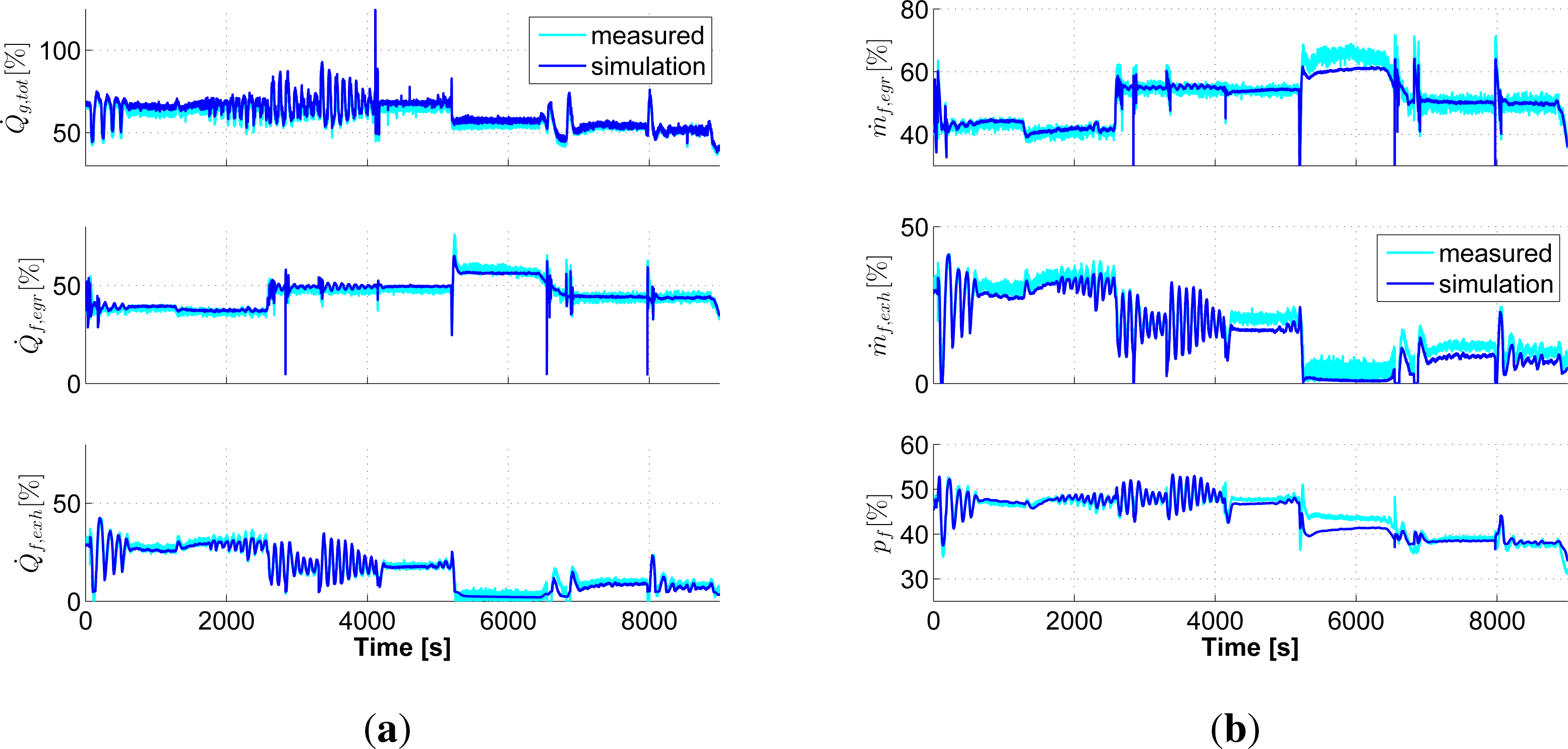
The measured signals used as input for the WHR system model are: the expander speed, bypass valves duty cycle, exhaust gas mass flow rate and temperature for both the EGR and EXH evaporator. Based on these input signals, the WHR system model predicts the heat flow rate through the system, the working fluid mass flow rate, the system pressure, the temperature and the power. For brevity, here, we show a few results that are related to the improved evaporator models.

In Figure 3, the heat flow through the system, mass flow rate and pressure are compared with the measurements. All of the heat flow rates are expressed relative to the maximum condenser cooling capacity. The working fluid mass flow rates ṁ_f,egr and ṁ_f,exh and system pressure p_f are expressed relative to the maximum values that the system can reach. To calculate the exhaust gas and working fluid heat flow rate for both evaporators, the following expressions are used:

$$\begin{array}{l}{\dot{Q}}_{\text{g}}={\dot{m}}_{\text{g}}{c}_{\text{pg}}\left(T_{\text{g},\text{in}}-T_{\text{g},\text{out}}\right)\\ {\dot{Q}}_{\text{f}}={\dot{m}}_{\text{f}}\left(h_{\text{f},\text{in}}-h_{\text{f},\text{out}}\right)\end{array}$$

(24)

where c_pg is the exhaust gas heat capacity. For brevity, in Figure 3a, we show the total exhaust heat flow rate, calculated as:

$${\dot{Q}}_{\text{g},\text{tot}}={\dot{Q}}_{\text{g},\text{egr}}+{\dot{Q}}_{\text{g},\text{exh}}+{\dot{Q}}_{\text{loss},\text{egr}}+{\dot{Q}}_{\text{loss},\text{exh}}$$

(25)

where Q̇_loss,egr and Q̇_loss,exh are the heat losses to the environment (see Equation (11a)). The exhaust gas heat flow rates Q̇_g,egr and Q̇_g,exh are transferred to the working fluid in the form of Q̇_f,egr and Q̇_f,exh, respectively. From the simulation results, we can see that heat flow rates through the system are well captured by the model on both the exhaust gas side and working fluid side, with an average error of 2%. Furthermore, the mass flow rates through both evaporators show good behavior. The average error is 3%, as well as the pressure dynamics, with an average error of 2%. The oscillations observed between 2000–4000 s are a consequence of the WHR control algorithm, which manipulates the bypass exhaust gas valve u_g1 due to cooling requirements. As can be seen, after 4000 s, a peak in the total exhaust gas heat flow rate is present that exceeds the condenser cooling capacity. However, this is for a short period of time, and thus, not visible in the working fluid heat flow rate, which could eventually lead to cooling issues.

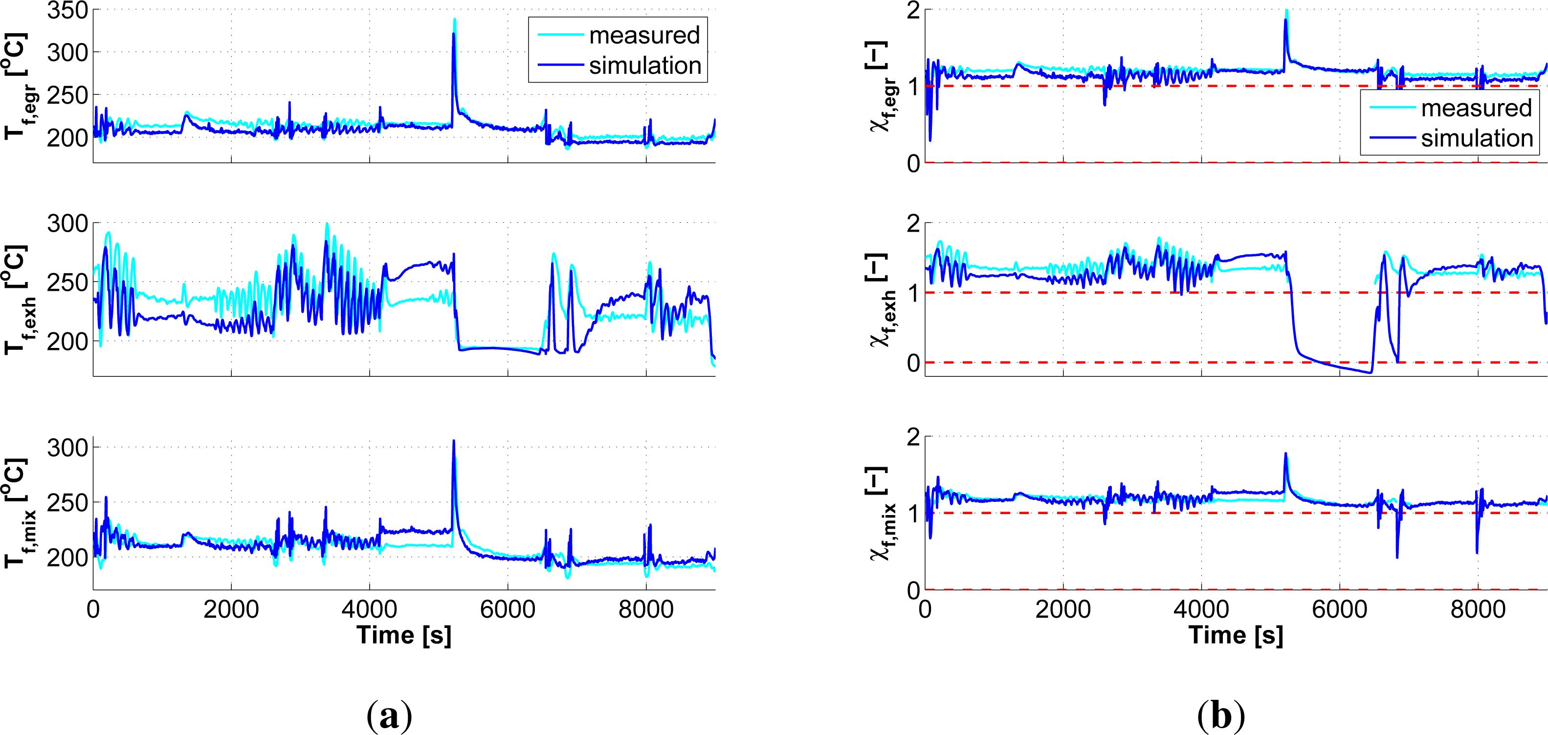
In Figure 4, the working fluid temperature and vapor fraction after the evaporators and mixing junction are compared with experimental data. The working fluid temperature after the EXH evaporator shows that there are differences as compared to the measurements. This follows from the applied data reconciliation techniques, which are not perfect and still result in some inaccuracies with respect to the energy conservation principle. To overcome this behavior, more accurate mass flow sensors are necessary. Unfortunately, this equipment was not available at the experimental set-up. Furthermore, the instrumentation to measure the vapor fraction was not available. However, in the liquid region (χ ≤ 0) and vapor region (χ ≥ 1), the vapor fraction can be calculated based on the measured temperature and pressure. The two-phase behavior can be validated by observing at which moment the working fluid switches from the vapor state to the two-phase state and back at the evaporator outlet. This behavior can be seen for the EXH evaporator between 5000–7000 s, where the vapor fraction χ_f,exh drops significantly due to the low heat input (see the corresponding Q̇_f,exh in Figure 3a).

The model prediction error is calculated using the following expression:

$$e=100\cdot \frac{\left|y_{\text{sim}}-y_{\text{meas}}\right|}{y_{\text{max}}-y_{\text{min}}}$$

(26)

where y_sim is the output to be compared, while y_max and y_min are the outputs at maximum and minimum engine thermal load, respectively. The resulting average and maximum error for the heat flow rate, mass flow rate, system pressure and temperature are summarized in

Table 1. Summary of the model prediction error and improvement compared with data from [17].

Symbol	Error		Improvement
	Average	Maximum	Average	Maximum
Q̇f	2%	4%	-	2%
ṁf	3%	7%	-	-
pf	2%	3%	-	1%
Tf	4%	13%	2%	7%

.

Compared to the previous model, we first see that the working fluid temperature prediction error decreased on average by 2%, while the maximum error decreased by 7%. This indicates that both the steady-state and dynamic behaviors of the evaporators are improved. For the mass flow rate, there is no improvement, since the pump and the valve models are kept the same. Furthermore, there is insignificant improvement for the average heat flow rate and system pressure error. However, due to the improved EGR and EXH evaporator models, the maximum heat flow rate and system pressure error decreased by 2% and 1%, respectively.

4. Control Design

In this section, the control objective is presented, followed by the model for control and the problem formulation in the model predictive control framework.

4.1. Control Objective

Based on Equation (13), let us denote the vapor fraction after the EGR and EXH evaporator with χ_f,egr and χ_f,exh. Using Equation (15), the vapor fraction downstream of the mixing junction is given by:

$${\chi }_{\text{f},\text{mix}}=\frac{{\dot{m}}_{\text{f},\text{egr}}{\chi }_{\text{f},\text{egr}}+{\dot{m}}_{\text{f},\text{exh}}{\chi }_{\text{f},\text{exh}}}{{\dot{m}}_{\text{f},\text{egr}}+{\dot{m}}_{\text{f},\text{exh}}}$$

(27)

In Figure 5, the control scheme is illustrated. The control input is u = [u_egr  u_exh]^⊤; the output is y = [χ_f,egr  χ_f,exh]^⊤; and the engine disturbance w = [Q̇_g,egr  Q̇_g,exh  ω_eng]^⊤. The controller design objective can now be formulated as the synthesis of a control algorithm that maximizes the WHR system output power while guaranteeing safe operation, i.e., χ_f,mix ≥ 1, in the presence of highly dynamic engine disturbances. However, an optimization problem that maximizes power with χ_f,mix ≥ 1 gives a non-unique global solution as a function of control input u. This could lead to excessive system actuation [21]. Additionally, in order to avoid infeasibility during optimization, the output constraints need to be included as soft constraints, which requires additional optimization variables. Thus, the problem complexity increases. To avoid these undesired effects while satisfying the safe operation requirement, here, we use a particular solution, in which the vapor quality after both evaporators indicates vapor, i.e., [χ_f,egr  χ_f,exh]^⊤ ≥ [1  1]^⊤. The expander is able to cope with working fluid in the two-phase state. Thus, for shorts periods of time, we assume a vapor fraction limit of 0.9 at the expander inlet.

The WHR system efficiency increases as the system operates closer to the safety margin [10], i.e., χ_f,egr = χ_f,exh = χ_f,mix = 1. Consequently, based on simulation results, the WHR output power is shown to reach its maximum at the safety margin [21]. Thus, for maximum output power, the controller design objective reduces to the synthesis of a control algorithm with good disturbance rejection properties that allows operation close to the safety limit.

4.2. Model for Control Design

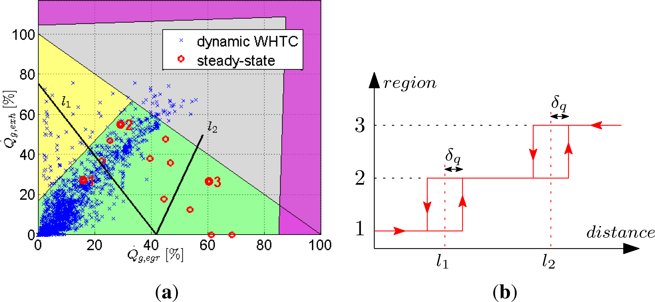
For control design, a low-computational model that captures the WHR system dynamics is necessary. However, the developed high-fidelity WHR system model has around 150 states and is highly nonlinear, mainly due to the two-phase phenomena. Therefore, the model is linearized and reduced around a representative set of operating conditions. In Figure 6a, we show the steady-state WHR system operating area, including limitations: the sum of Q̇_g,egr and Q̇_g,exh is limited to 100% by the condenser cooling power; ethanol decomposition can occur at a temperature higher than 280 °C, and emissions can increase due to the low exhaust gas flow through the EGR valve. These limitations are expressed in the steady state, and thus, they can be violated for short periods of time, especially during transients. The resulting WHR system operating area is shown in green in Figure 6a.

Within the WHR system operating area, three linearization points are selected (see Figure 6a with numbers) that are shown to be sufficient in describing the WHR system dynamics [16]. The points are selected close to the boundaries for emissions and condenser limitation, where the system is expected to operate more often. This is seen from a World Harmonized Transient Cycle and steady-state measurements that also motivate the switching lines choice l₁ and l₂.

The three corresponding linear models are of high order, because they retain the same number of states as the high-fidelity model. To use these models for control, model reduction techniques based on balanced truncation are used. A model order of n = 7 is chosen, such that the error system ‖G − G_r‖_∞ satisfies:

$${\Vert G-G_{\text{r}}\Vert }_{\infty }\le 2\left({\sigma }_{n+1}+{\sigma }_{n+2}+\dots +{\sigma }_m\right)$$

(28)

where G is the full linear model of order m, G_r is the reduced linear model of order n and σ are the singular values of G. The reduced order state-space linearized model in discrete time is:

$$\begin{array}{c}x(k+1)=A_{i}x(k)+B_{i,u}u(k)+B_{i,w}w(k)\\ y(k)=C_{i}x(k),\hspace{0.17em}\hspace{0.17em}\hspace{0.17em}\hspace{0.17em}\hspace{0.17em}\hspace{0.17em}\hspace{0.17em}i=\{1,2,3\}\end{array}$$

(29)

where A_i ∈ ℝ^n×n, B_i,u ∈ ℝ^n×q, B_i,w ∈ ℝ^r×n, x ∈ ℝⁿ, u ∈ ℝ^p, w ∈ ℝ^q, y ∈ ℝ^r.

The three reduced order models are integrated within the control scheme using a switching mechanism with hysteresis, as shown in Figure 6b. The switching mechanism indicates the active controller based on the EGR and EXH heat flow rates from the engine. This is achieved by monitoring the distance between the switching lines l₁, l₂ and the point that expresses the current EGR and EXH heat flow rate. A parameter δ_q that defines the hysteresis is introduced to avoid chattering around the switching lines. From simulation results, we conclude that δ_q = 14.5% gives good switching behavior without chattering.

4.3. Linear Model Predictive Control

The control inputs u(k) = [u_egr(k)  u_exh(k)]^⊤, at time k, are computed by an MPC controller. The controller consists of a state estimator and an optimizer (see Figure 5). The state estimator is used to obtain estimates of x(k) from the output y(k) = [χ_f,egr(k)  χ_f,exh(k)]^⊤ computed from the measurements. To improve the state estimation, the engine disturbances w(k) are assumed to be measured.

The optimizer solves a linear optimization problem that minimizes a cost function J subject to constraints. As the objective is to have good disturbance rejection, the cost function J penalizes deviations of the predicted controlled outputs ŷ(k + i) from a constant reference r(k + i) and changes of the inputs Δu(k + i). The penalty matrices W_y and W_Δu are constant inside each operating region of the WHR system. The predictions are expressed in terms of Δu(k + i) = u(k + i) − u(k + i − 1), and the cost function is defined as:

$$J(k)=\sum _{i=0}^{N_{\text{y}}-1}{\Vert r(k+i+1)-\widehat{y}(k+i+1)\Vert }_{W_{\text{y}}}^2+\sum _{i=0}^{N_u-1}{\Vert \mathrm{\Delta }u(k+i)\Vert }_{W_{\mathrm{\Delta }u}}^2,\hspace{0.17em}\hspace{0.17em}\hspace{0.17em}\hspace{0.17em}\hspace{0.17em}\hspace{0.17em}\hspace{0.17em}{N}_{\text{u}}\le N_{\text{y}}$$

(30)

where N_y is the prediction horizon and N_u is the control horizon. The cost function J(k) is obtained based on the reduced order linear model, which is used to predict the behavior of the plant, starting at the current time k, over a future prediction horizon N_y. This predicted behavior depends on the assumed input trajectory u(k + i) over a control horizon N_u and measured output y(k) and disturbance w(k). The input increments Δu(k + i) = 0 for i ≥ N_u, i.e., u(k + i) = u(k + N_u − 1) for all i ≥ N_u. In Equation (30), ${\Vert \cdot \Vert }_W^2$ denotes the weighted two-norm squared, i.e., ${\Vert x\Vert }_W^2=x^{\top }{W}^{\top }Wx$.

At each time k ∈ ℤ₊, we estimate the system state x(k) and solve the following optimization problem (this is often called a receding horizon principle):

Problem 1.

$$\underset{\mathrm{\Delta }u(k),\dots ,\mathrm{\Delta }u(k+N_u-1)}{\text{min}}J(k)$$

(31)

subject to Equation (29) and:

$$0\le u(k+i)\le 100,\hspace{0.17em}\hspace{0.17em}\hspace{0.17em}\hspace{0.17em}i=0,\dots ,N_y-1$$

(32)

The control action sent to the system is u(k) = u(k − 1) + Δu^*(k), where Δu^*(k) is the first element of the optimal sequence obtained by solving Problem 1. For state estimation, a general linear state observer [22] is designed based on the measured plant output, which gives the state estimate x̂ through a gain matrix. The gain matrix is designed using well-known Kalman filtering techniques.

For each region in the operating WHR area, an MPC controller is designed. All three MPC controllers receive the current manipulated variable and output signals, for their state estimates. During switching, the state estimator can experience bumps, because the model reduction does not preserve the same states for each region. However, by penalizing the input increments Δu(k + i|k) in the optimization Problem 1, these effects are mitigated and aggressive plat actuation is avoided.

4.4. Nonlinear Model Predictive Control

In this section, a nonlinear model predictive control (NMPC) is developed using the high-fidelity WHR system model. First, let us denote the high-fidelity WHR system using the general form of a non-linear system:

$$\begin{array}{l}\dot{x}=f(x,u,w)\\ y=g(x)\end{array}$$

(33)

where x is the state vector, u the control input, w the disturbance vector and y the model output. Then, at each time step k ∈ ℤ₊, the NMPC strategy solves the following optimization problem:

Problem 2.

$$\underset{u(k),\dots ,u(k+N_u-1)}{\text{min}}J(k)$$

(34)

subject to Equation (33) and:

$$0\le u(k+i)\le 100,\hspace{0.17em}\hspace{0.17em}\hspace{0.17em}\hspace{0.17em}\hspace{0.17em}\hspace{0.17em}i=0,\dots ,N_y-1$$

(35)

The NMPC uses the same prediction horizon N_y and control horizon N_u as the linear MPC. However, note that Problem 2 computes directly the control input u(k) over the control horizon N_u and not the control input increment Δu(k). Moreover, a state estimator and a switching mechanism are not necessary, since the control model and the high-fidelity model are identical.

The reason for developing an NMPC strategy is only for comparison purposes, since the algorithm is computationally expensive and, thus, is not feasible for online implementation.

5. Simulation Results and Discussion

To evaluate the MPC strategy, measurements from a Euro VI heavy-duty diesel engine are used. The control strategy is tested on a simple stepwise cycle and then on a cold-start World Harmonized Transient Cycle (WHTC) that covers typical driving conditions: urban, rural and highway. As a benchmark, a classical PI controller is used [16], as well as a nonlinear MPC (NMPC) strategy. The PI control objective is to manipulate the control input u, such that the evaporator’s outlet temperature follows a predefined reference temperature. This reference temperature is the ethanol saturation temperature plus a safety margin of 10 °C. The simulation environment is MATLAB/Simulink^® from The Mathworks Inc., Massachusetts, MA, USA. The MPC strategy is implemented using the model predictive control Toolbox, while the NMPC strategy uses a sequential quadratic programming (SQP) solver.

The controller sampling time is T_s = 0.4 s, which yields an acceptable approximation of the system dynamics. The prediction horizon is N_y = 45, and the control horizon is N_u = 4 time steps. The prediction horizon of 18 s is chosen, so that the most important system dynamics within the engine operating area are captured. The control horizon of 1.6 s follows from the fact that larger values do not considerably improve the performance, while the computational complexity increases significantly. The corresponding weighting matrices are:

$$\begin{array}{ll}{\text{MPC}}_{\{1,2,3\}}:\hfill & W_{\text{y}}=\left\{\text{diag}(0.8,0.8),\hspace{0.17em}\text{diag}(0.9,0.9),\hspace{0.17em}\hspace{0.17em}\text{diag}(0.8,0.9)\right\},\hfill \\ \hfill & W_{\mathrm{\Delta }u}=\left\{\text{diag}(0.05,0.05),\hspace{0.17em}\hspace{0.17em}\text{diag}(0.1,0.1),\hspace{0.17em}\hspace{0.17em}\text{diag}(0.2,0.2)\right\},\hfill \\ \text{NMPC}:\hfill & W_{\text{y}}=\text{diag}(0.9,0.8),\hfill \\ \hfill & W_u=\text{diag}({10}^{-5},{10}^{-5})\hfill \end{array}$$

(36)

For the MPC strategy, the weighting matrices are tuned for a stepwise cycle, such that a good trade-off is obtained between control effort and robustness to model uncertainty. However, using these settings, the controller is shown to perform well also for other type of cycles, such as a WHTC. For the NMPC strategy, a similar weighting is chosen for W_y. Since the NMPC optimization is performed subject to the high-fidelity model in Equation (33), the weighting W_u is chosen small to allow more control freedom.

5.1. Stepwise Cycle

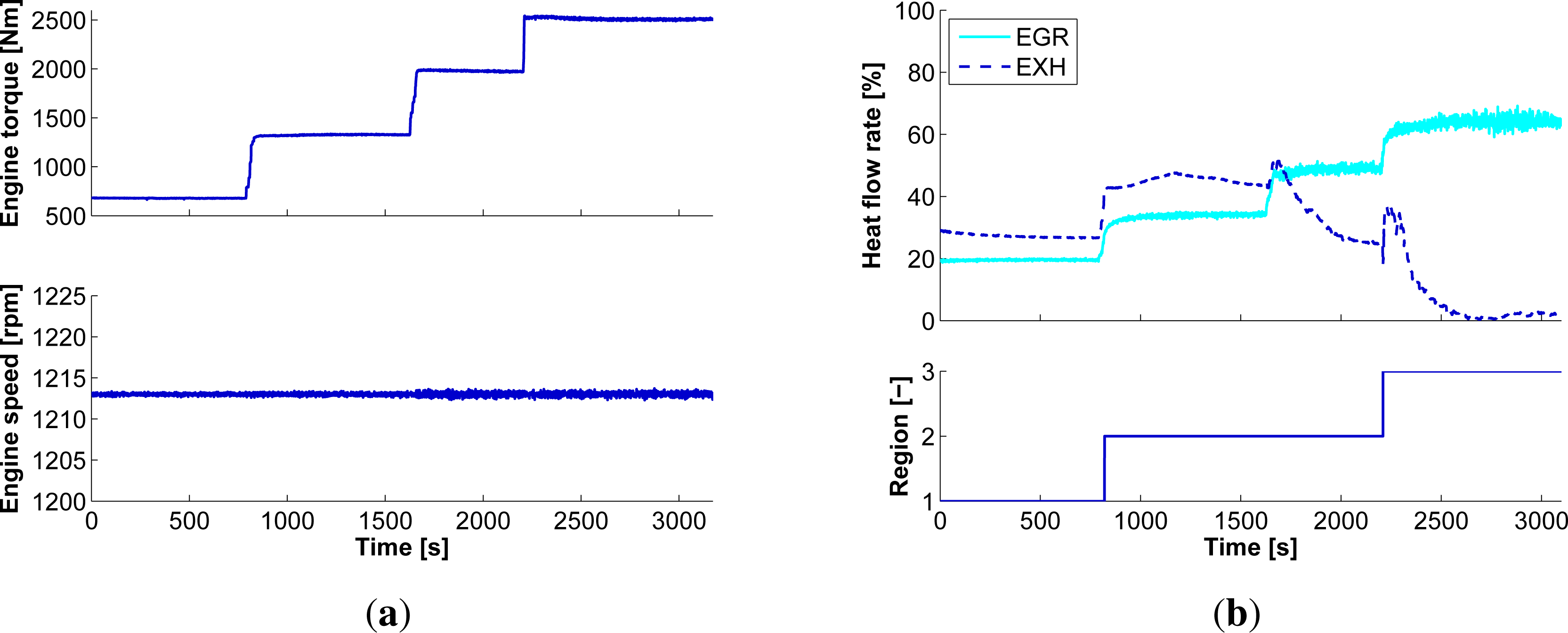
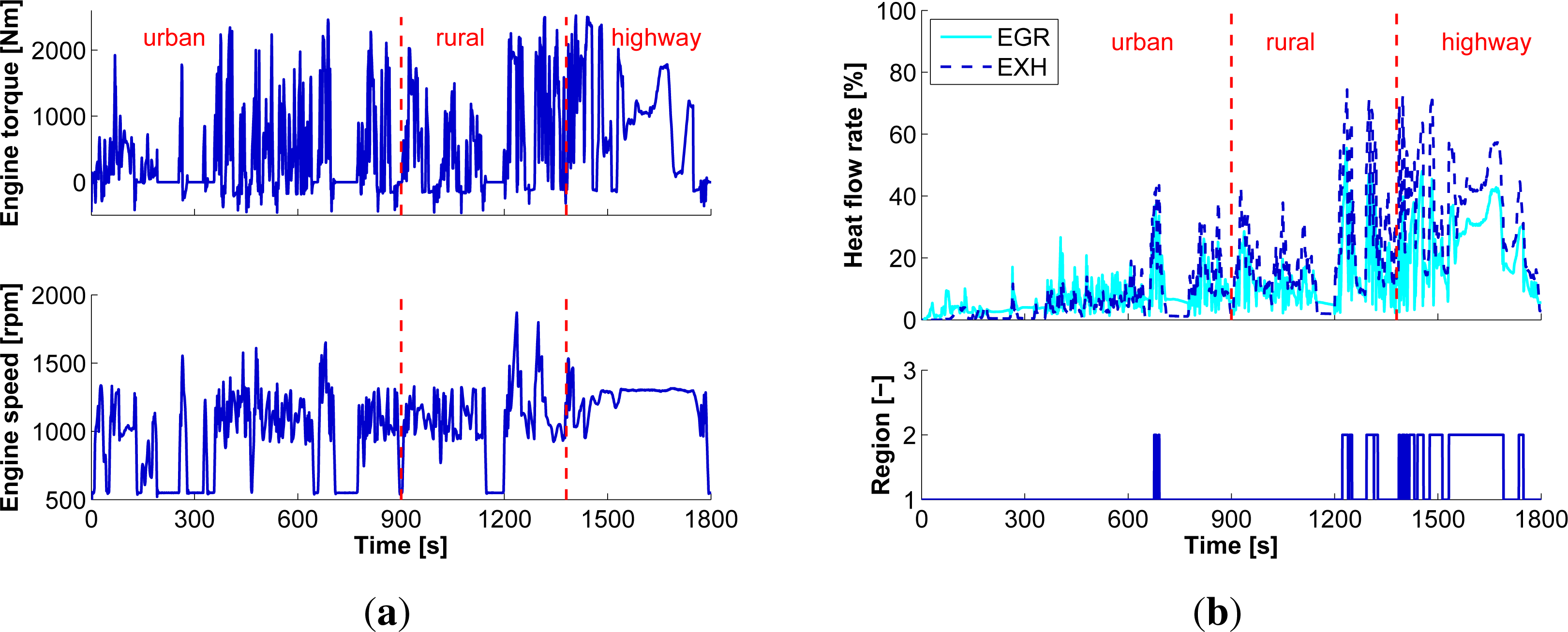
In this cycle, illustrated in Figure 7a, the engine torque is varied stepwise within the complete operating area, i.e., 500–2600 N·m, while the speed is kept constant at 1213 rpm. From the WHR system perspective, the engine torque and speed translates into EGR and EXH heat flow rate (see Figure 7b). The EGR and EXH heat flow rate together with the engine speed are the main disturbances for the WHR system, besides other disturbances, such as ambient temperature and ethanol temperature from the reservoir. The operating region is determined based on the EGR and EXH heat flow rate outside the controller. All three controllers become active with no chattering during switching, which could lead to instability. This indicates a good switching behavior of the switching mechanism with hysteresis.

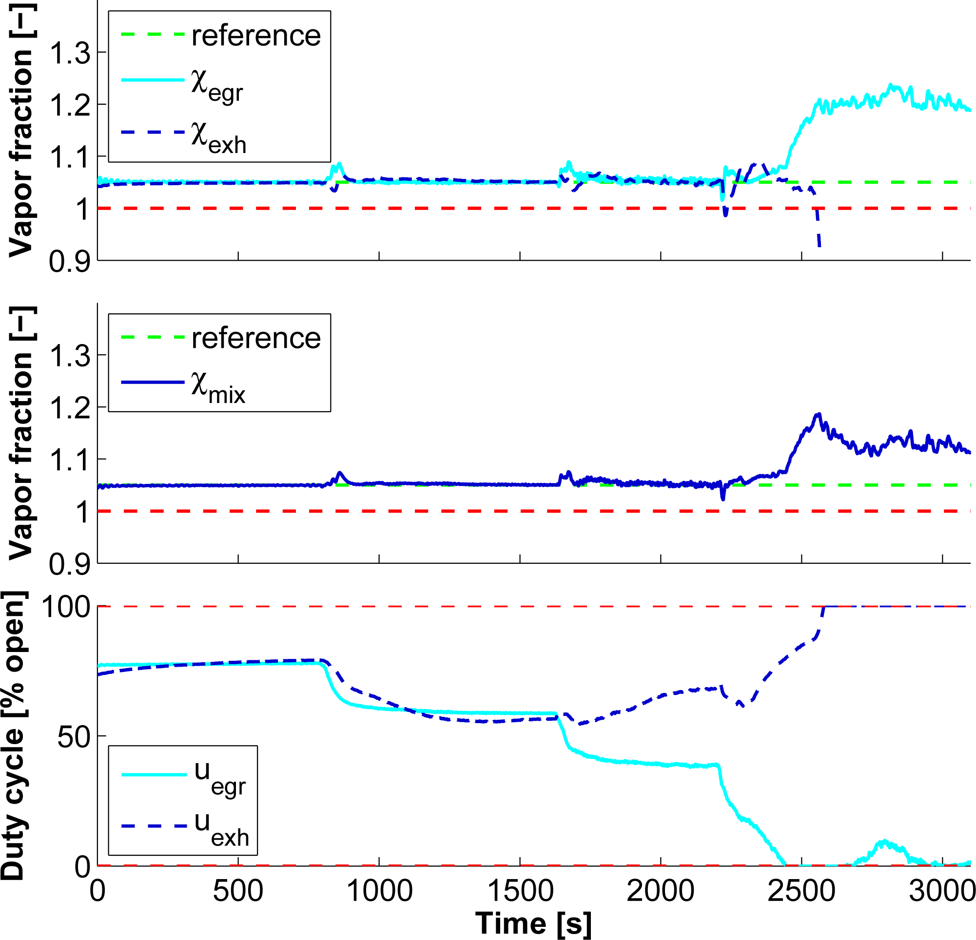
In Figure 8, we show the vapor fraction after the EGR and EXH evaporator, as well as after the mixing junction. The reference r for the controller is set to a constant value of 1.05 superheat for both evaporators. From Equation (13), the superheat in temperature corresponding to this vapor fraction varies as a function of pressure from 10 °C to less than 5 °C as the pressure reaches its maximum. After the mixing junction, a good disturbance rejection is obtained, with ±5% maximum deviation from the specified reference r. Starting from 2400 s, the control inputs reached the limits (see the lower plot in Figure 8), i.e., u_egr = 0% (fully closed) and u_exh = 100% (fully opened). Thus, the output is indeed no longer able to follow the reference. The reason comes from the engine heat flow rate: at the EGR evaporator, the exhaust gas heat flow rate reached more than 60% while at the EXH evaporator, it dropped close to zero due to u_g2 actuation to avoid exceeding the condenser cooling capacity. However, depending on the situation, the vapor fraction after the mixing junction can still show the vapor state, and therefore, mechanical power is delivered, despite the control input that hit the constraint.

5.2. World Harmonized Transient Cycle

To validate and quantify the performance of the developed control strategy, a highly dynamic cold-start World Harmonized Transient Cycle (WHTC) is used (Figure 9a). This is an 1800 s cycle that consists of urban, rural and highway driving conditions. The WHTC is a challenging cycle due to a highly dynamic behavior that includes also the heat-up phase of the engine and WHR system. The engine disturbances from such a cycle are illustrated in Figure 9b. The switching signal indicates that only Regions 1 and 2 are reached.

For comparison, we use two additional control strategies: a classical PI control scheme [16] and an NMPC strategy described in Section 4. The results for these three control strategies are shown in Figure 10. For brevity, we only show the vapor fraction after the mixing junction.

During the first 1200 s, the WHR system is heating up, and therefore, no vapor state is encountered after the mixing junction. Note, however, that for each evaporator, the heat-up period is different, up to 600 s for the EGR evaporator and 1200 s for the EXH evaporator. The exhaust evaporator takes longer to heat-up due to more mass and the aftertreatment system located upstream. The difference in heat-up period can be observed also from the period of time the control input u_egr and u_exh are on the constraint.

The objective of all three controllers is to maintain vapor and to be as close as possible to χ_f,egr = χ_f,exh = 1 for maximum output power. However, due to highly dynamic disturbances and the limitations of the control input, maintaining the vapor state is challenging. The main reasons for introducing an NMPC controller are: first, to verify how good is the control strategy if the WHR system model is exactly known, and second, what the global control input solution is. From the simulation results, we found that the global solution is difficult to obtain, since the system is highly nonlinear with local minima over the prediction horizon. Thus, the NMPC solution is sensitive to the initial condition for the optimization Problem 2. Here, for initialization of the NMPC strategy, we used the MPC solution. As a result, the NMPC strategy corrects for the modeling errors between the reduced order linear model and the high-fidelity model.

At first instance, all three controllers seem to behave quite similarly, especially the MPC and NMPC control strategies. To quantify the performance of each controller, we use two indicators: the time in the vapor state t_v and the recovered thermal energy U over the complete cycle.

The performance indicators are define as follows:

$$\text{Time}\hspace{0.17em}\text{in}\hspace{0.17em}\text{vapor}\hspace{0.17em}\text{state}:t_{\text{v}}=T_{\text{s}}\sum _0^{t_f}\left({\chi }_{\text{mix}}\ge 1\right)$$

(37)

$$\text{Thermal}\hspace{0.17em}\hspace{0.17em}\text{energy}:\hspace{0.17em}\hspace{0.17em}U={\int }_0^{t_{\text{v}}}{P}_{\text{whr}}(t)dt$$

(38)

where t_f is the total cycle time and P_whr(t) is the instantaneous WHR system net output power. The instantaneous output power P_whr(t) and the recovered energy U are calculated only when the safety requirement χ_mix ≥ 1 is satisfied. In the case that the safety requirement is not fulfilled, i.e., χ_mix < 1, the expander needs to be bypassed to avoid damage.

From Figure 11, we can see that the MPC controller outperforms the PI controller in terms of time in the vapor state and recovered thermal energy, with approximately 15%. The NMPC strategy improves the considered performance indices by 10% as compared to the MPC strategy. This result gives an indication about the model uncertainty used within the MPC strategy. Despite the improved result, the NMPC controller has several drawbacks. First, the computational complexity is significant, which makes the NMPC scheme not feasible for real-time implementation. Second, it can converge to local minima, resulting in worse control behavior than with a linear MPC. As a solution, an NMPC algorithm that uses global solvers can be considered; however, the computational complexity will grow even more.

6. Conclusions and Future Research

The modeling and control of a waste heat recovery system for a Euro-VI heavy-duty truck engine was considered. The exhaust gas energy is recovered by means of two parallel evaporators. To generate power, an expander is used, mechanically coupled with the pumps to the engine crankshaft. The main conclusions of this paper are summarized in what follows.

(1)

The existing WHR system model was improved by including enhanced evaporator models. The model combines the finite difference modeling approach with a moving boundary one and, thus, captures multiple phase transitions along a single pipe flow.

(2)

A switching model predictive control strategy was designed, to guarantee the safe operation of the WHR system. The proposed control strategy performance is demonstrated on a highly dynamic cold-start World Harmonized Transient Cycle. Simulation results showed improved performance for the proposed MPC strategy in terms of vapor time and recovered thermal energy by 15%, as compared to a classical PI controller.

(3)

A nonlinear model predictive control was developed to demonstrate that control performance can be improved by approximately 10% in the case that the model of the system is exactly known.

(4)

One limitation of the proposed MPC strategy is the need of vapor fraction measurement equipment or an estimator to make the method applicable in practice.

Future work will focus on vapor fraction estimation and on experimental demonstration of the proposed MPC strategy. Furthermore, the supervisory control strategy [23] that combines energy and emission management will be extended by considering the proposed WHR control strategy.

References

- Endo, T.; Kawajiri, S.; Kojima, Y.; Takahashi, K.; Baba, T.; Ibaraki, S.; Takahashi, T.; Shinohara, M. Study on maximizing exergy in automotive engines. In Proceedings of the SAE World Congress and Exhibition, Detroit, MI, USA, 16–19 April 2007.
- Charles, S.; Christopher, D. Review of organic Rankine cycles for internal combustion engine exhaust waste heat recovery. J. Appl. Therm. Eng 2013, 51, 711–722. [Google Scholar]
- Zhang, J.H.; Zhou, Y.L.; Hou, G.L.; Fang, F. Generalized predictive control applied in waste heat recovery power plants. J. Appl. Energy 2013, 102, 320–326. [Google Scholar]
- Yang, K.; Zhang, H.; Song, S.S.; Zhang, J.; Wu, Y.T.; Zhang, Y.Q.; Wang, H.J.; Chang, Y.; Bei, C. Performance analysis of the vehicle diesel engine-ORC combined system based on a screw expander. Energies 2014, 7, 3400–3419. [Google Scholar]
- Dolz, V.; Novella, R.; Garcia, A.; Sanchez, J. HD diesel engine equipped with a bottoming Rankine cycle as a waste heat recovery system. Part 1: Study and analysis of the waste heat energy. J. Appl. Therm. Eng 2012, 36, 269–278. [Google Scholar]
- Katsanos, C.; Hountalas, D.; Pariotis, E. Thermodynamic analysis of a Rankine cycle applied on a diesel truck engine using steam and organic medium. J. Energy Convers. Manag 2012, 60, 68–76. [Google Scholar]
- Hounsham, S.; Stobart, R.; Cooke, A.; Childs, P. Energy recovery systems for engines. In Proceedings of the SAE World Congress and Exhibition, Detroit, MI, USA, 14–17 April 2008.
- Quoilin, S.; Aumann, R.; Grill, A.; Schuster, A.; Lemort, V.; Spliethoff, H. Dynamic modeling and optimal control strategy of waste heat recovery organic Rankine cycles. J. Appl. Energy 2011, 88, 2183–2190. [Google Scholar]
- Tona, P.; Peralez, J.; Sciarretta, A. Supervision and control prototyping for an engine exhaust gas heat recovery system based on a steam rankine cycle. In Proceedings of the 2012 IEEE/ASME International Conference on Advanced Intelligent Mechatronics, Kaohsiung, Taiwan, 11–14 July 2012; pp. 695–701.
- Xie, H.; Yang, C. Dynamic behavior of Rankine cycle system for waste heat recovery of heavy duty diesel engines under driving cycle. J. Appl. Energy 2013, 112, 130–141. [Google Scholar]
- Horst, T.; Rottengruber, H.; Seifert, M.; Ringler, J. Dynamic heat exchanger model for performance prediction and control system design of automotive waste heat recovery systems. J. Appl. Energy 2013, 105, 293–303. [Google Scholar]
- Peralez, J.; Tona, P.; Lepreux, O.; Sciarretta, A.; Voise, L.; Dufour, P.; Nadri, M. Improving the control performance of an organic rankine cycle system for waste heat recovery from a heavy-duty diesel engine using a model-based approach. In Proceedings of the 52nd IEEE Conference on Decision and Control, Firenze, Italy, 10–13 December 2013; pp. 6830–6836.
- Hou, G.; Hu, G.; Zhang, J. Supervisory Predictive Control of Evaporator in Organic Rankine Cycle (ORC) System for Waste Heat Recovery. In Proceedings of the 2011 International Conference on Advanced Mechatronic Systems, Zhengzhou, Henan, China, 11–13 August 2011; pp. 306–311.
- Zhang, J.; Zhang, W.; Guolian, H.; Fang, F. Dynamic modeling and multivariable control of organic Rankine cycles in waste heat utilizing processes. J. Comput. Math. Appl 2012, 64, 908–921. [Google Scholar]
- Wallace, M.; Das, B.; Mhaskar, P.; House, J.; Salsbury, T. Offset-free model predictive control of a vapor compression cycle. J. Process Control 2012, 22, 1374–1386. [Google Scholar]
- Feru, E.; Willems, F.; Rascanu, G.; de Jager, B.; Steinbuch, M. Control of Automotive Waste Heat Recovery Systems with Parallel Evaporators; International Federation of Automotive Engineering Societies (FISITA): Maastricht, The Netherlands, 2014. [Google Scholar]
- Feru, E.; Kupper, F.; Rojer, C.; Seykens, X.; Scappin, F.; Willems, F.; Smits, J.; de Jager, B.; Steinbuch, M. Experimental Validation of a Dynamic Waste Heat Recovery System Model for Control Purposes. In Proceedings of SAE 2013 World Congress and Exhibition, Detroit, MI, USA, 16–18 April 2013.
- Feru, E.; de Jager, B.; Willems, F.; Steinbuch, M. Two-phase plate-fin heat exchanger modeling for waste heat recovery systems in diesel engines. J. Appl. Energy 2014, 133, 183–196. [Google Scholar]
- Hou, G.; Bi, S.; Lin, M.; Zhang, J.; Xu, J. Minimum variance control of organic Rankine cycle based waste heat recovery. J. Energy Convers. Manag 2014, 86, 576–586. [Google Scholar]
- VDI-Gesellschaft Verfahrenstechnik und Chemieingenieurwesen. In VDI Heat Atlas; Springer: Berlin, Germany, 2010.
- Feru, E.; Willems, F.; de Jager, B.; Steinbuch, M. Model predictive control of a waste heat recovery system for automotive diesel engines. In Proceedings of the 18th International Conference on System Theory, Control and Computing, Sinaia, Romania, 17–19 October 2014.
- Lewis, F. Optimal Estimation; John Wiley & Sons, Inc: Michigan, MI, USA, 1986. [Google Scholar]
- Willems, F.; Kupper, F.; Rascanu, G.; Feru, E. Integrated energy and emission management for diesel engines with waste heat recovery using dynamic models. Oil Gas Sci. Technol. Rev. IFP Energ. Nouv 2014, 69, 1–16. [Google Scholar]