Control Strategies to Smooth Short-Term Power Fluctuations in Large Photovoltaic Plants Using Battery Storage Systems

Abstract
:1. Introduction
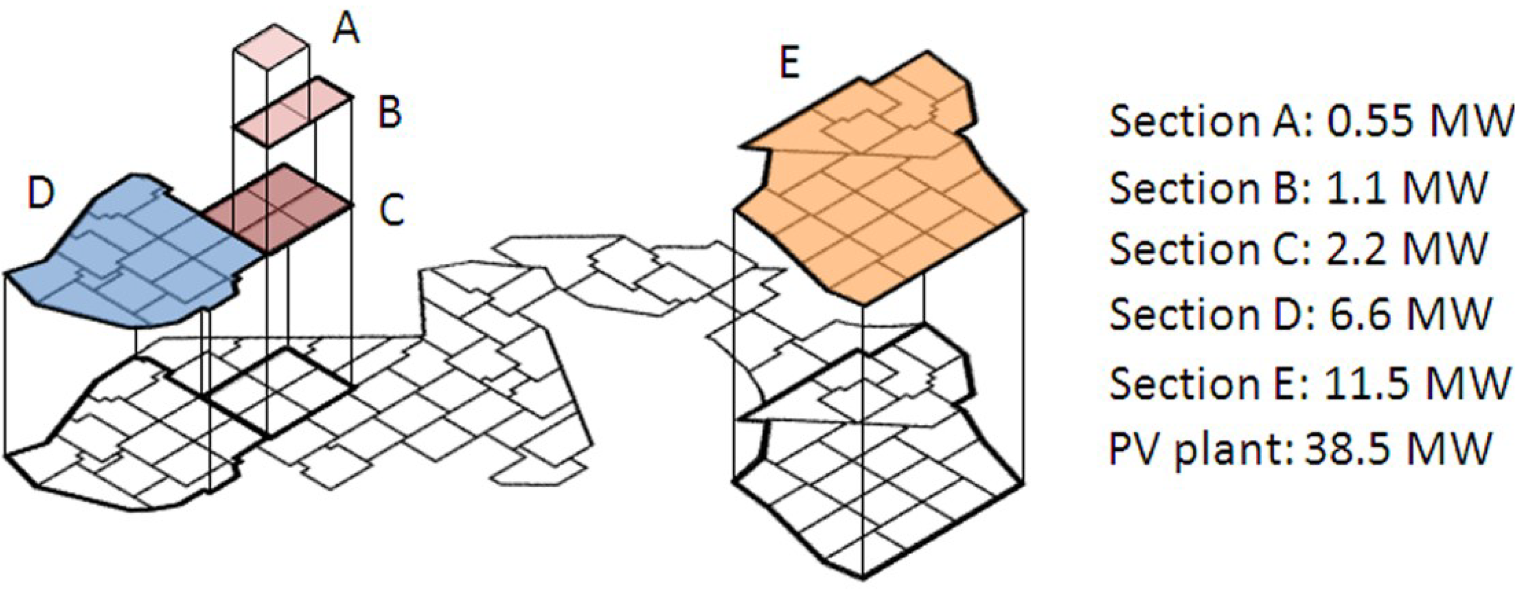
2. Database

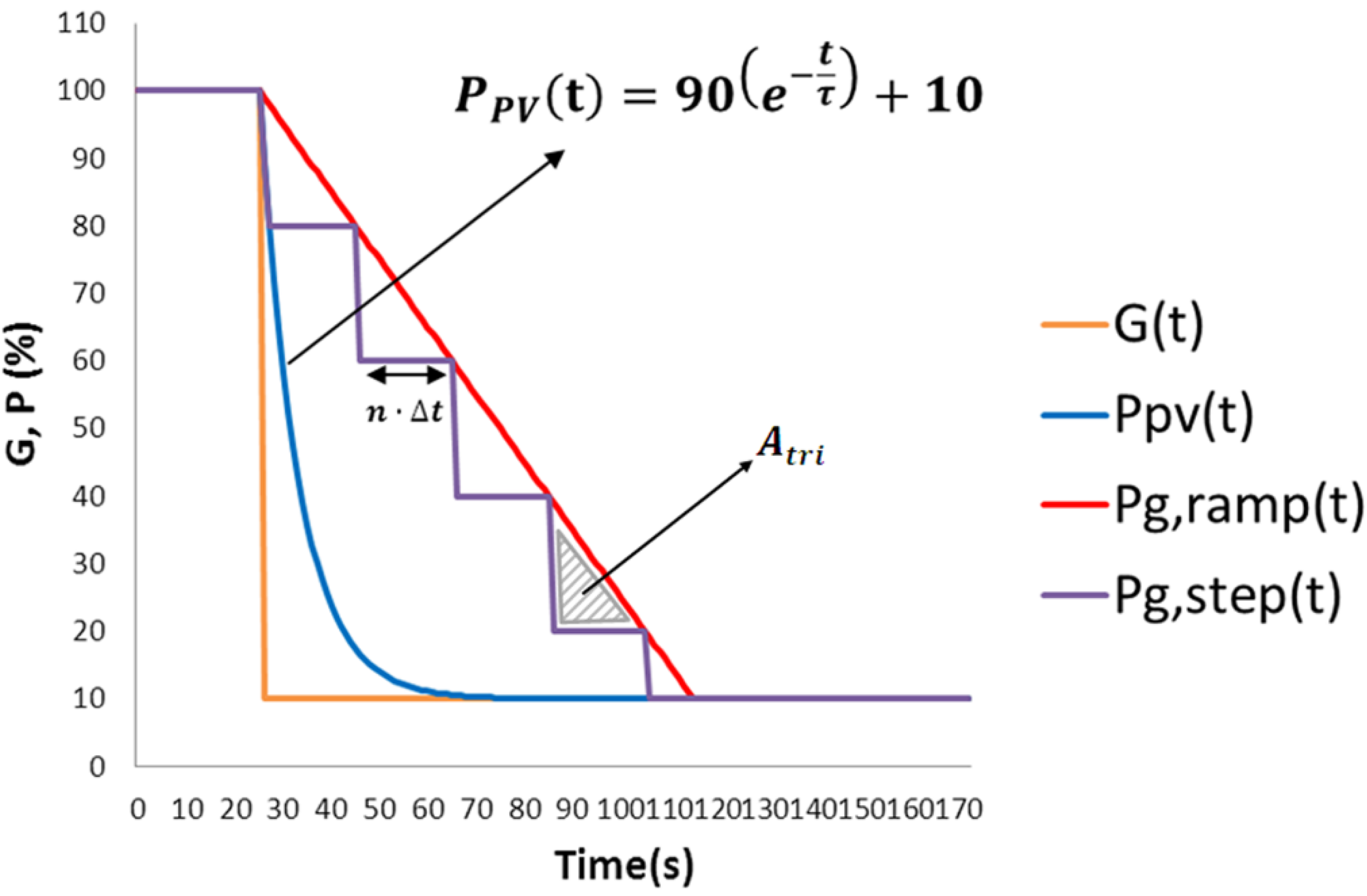
3. Power Fluctuations with No Energy Storage

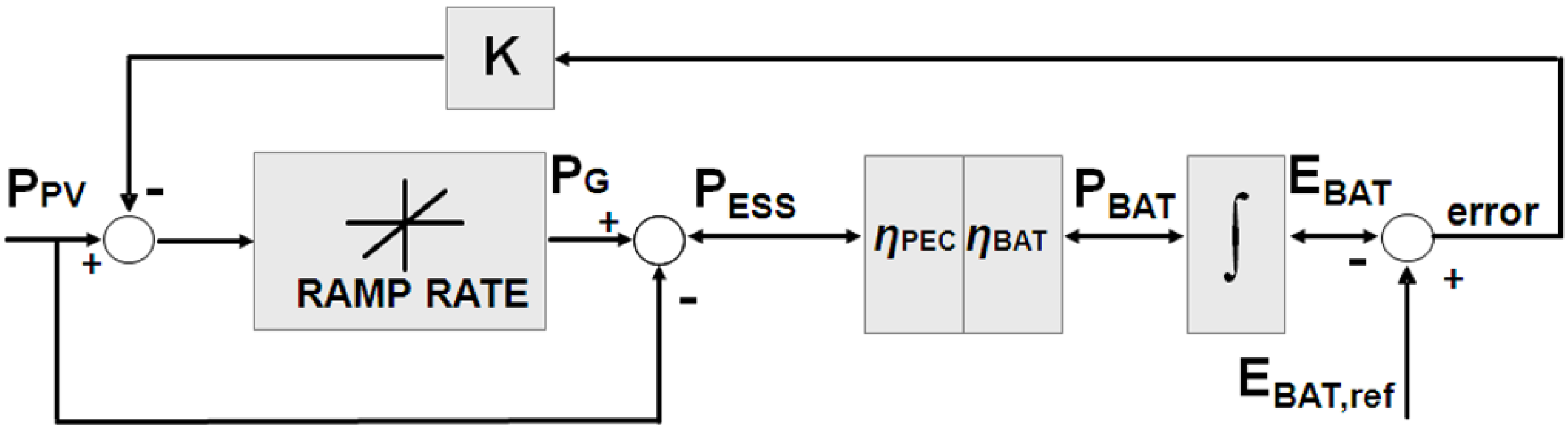
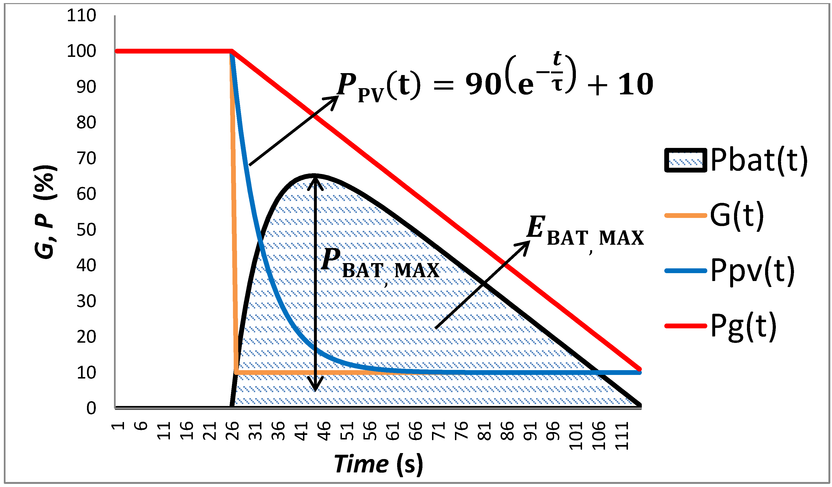
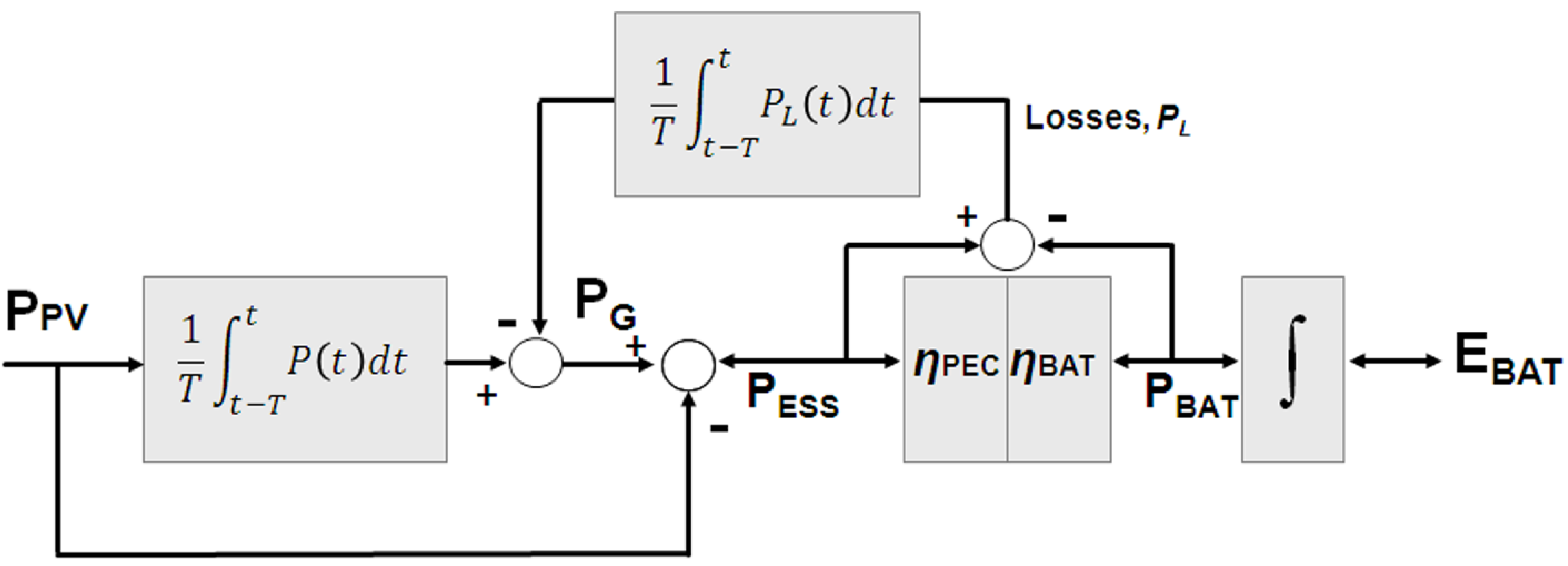
4. A Generic Strategy for Smoothing Fluctuations through Energy Storage


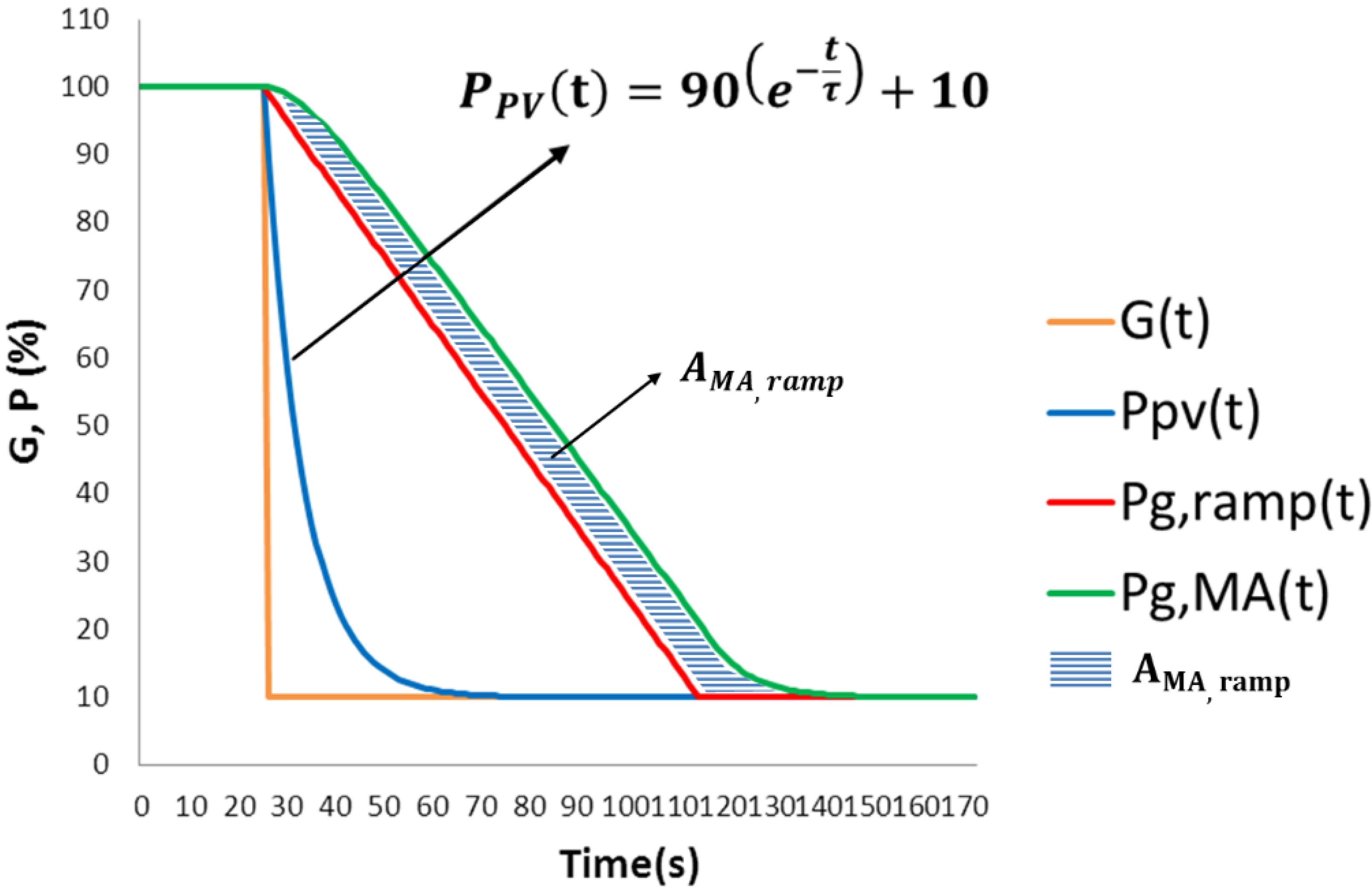
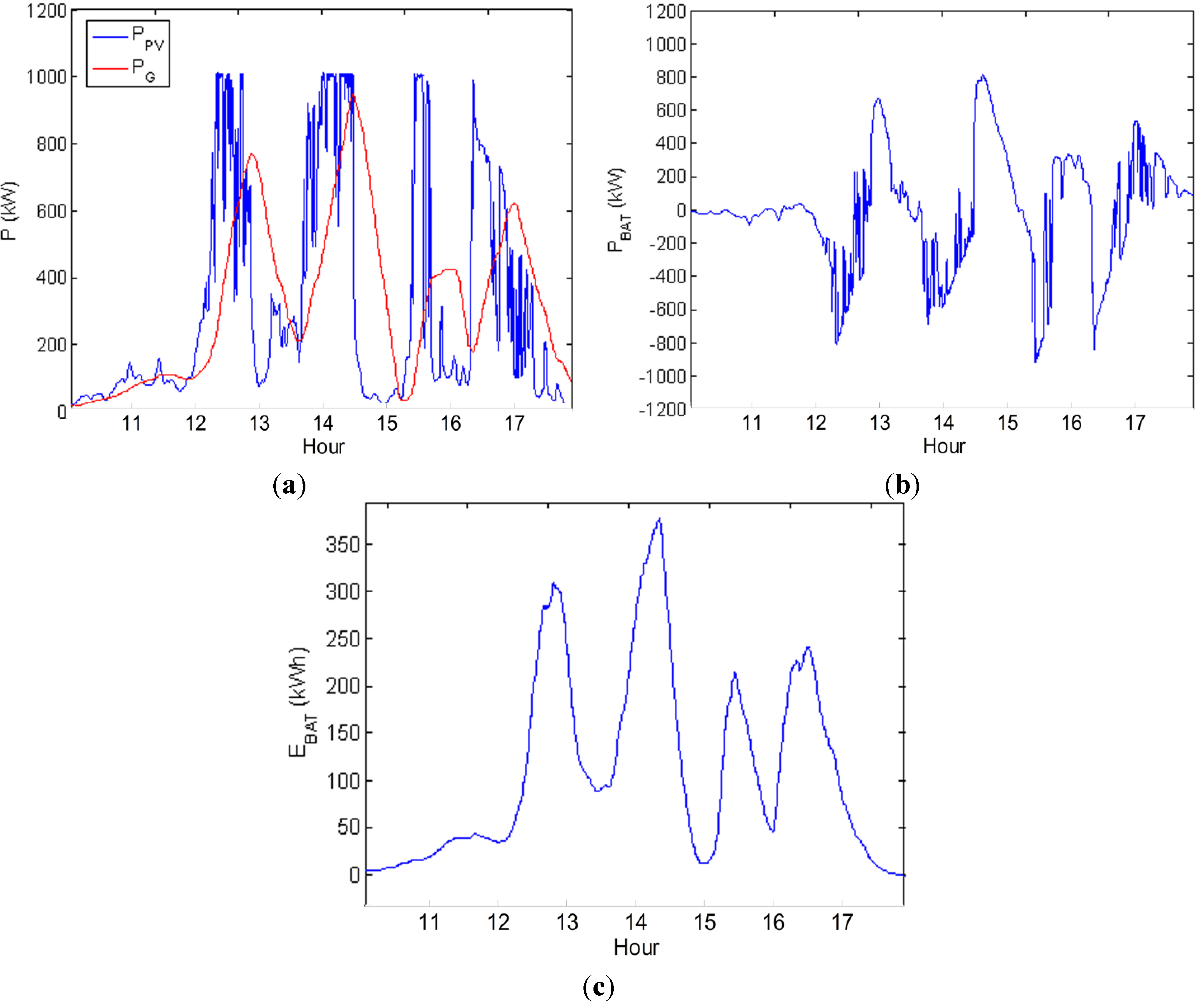
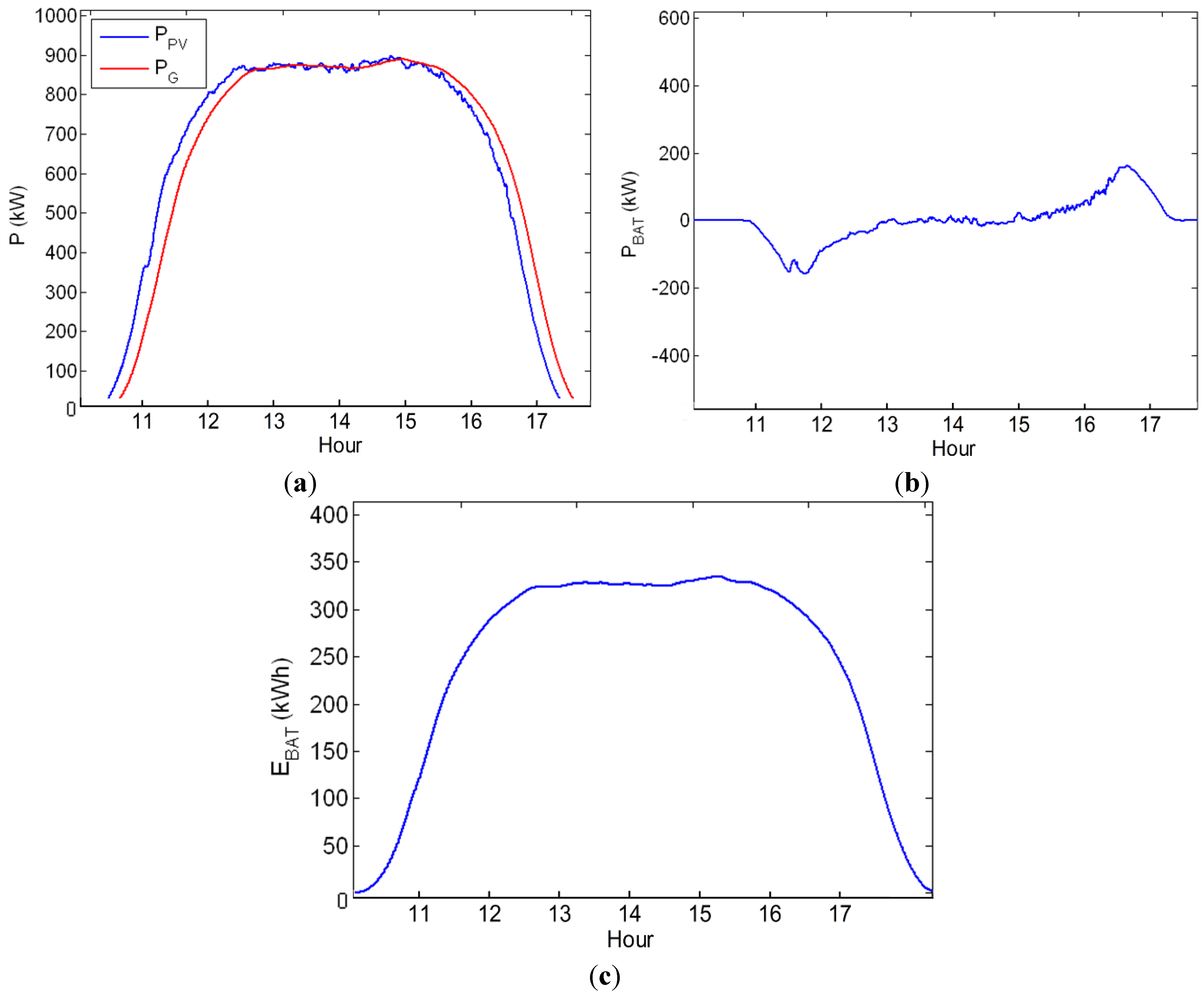
4.1. Ramp Control Strategy


4.2. Moving-Average Strategy


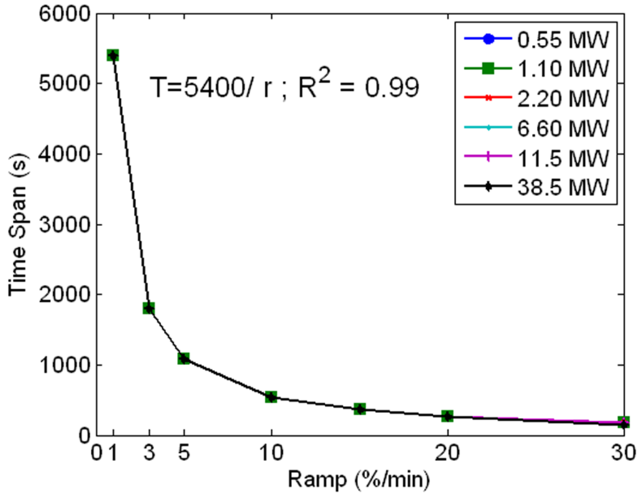
Selection of Time Window T for the Moving-Average Strategy

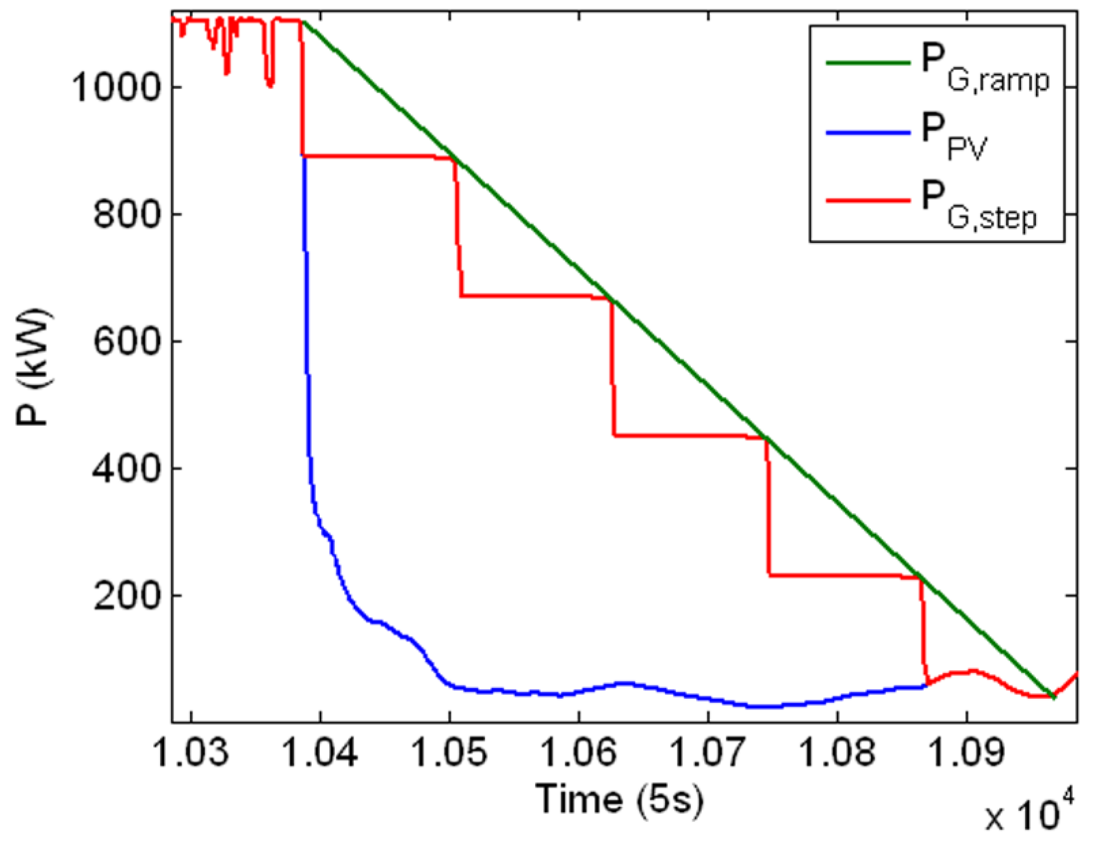
4.3. Step-Rate Control Strategy


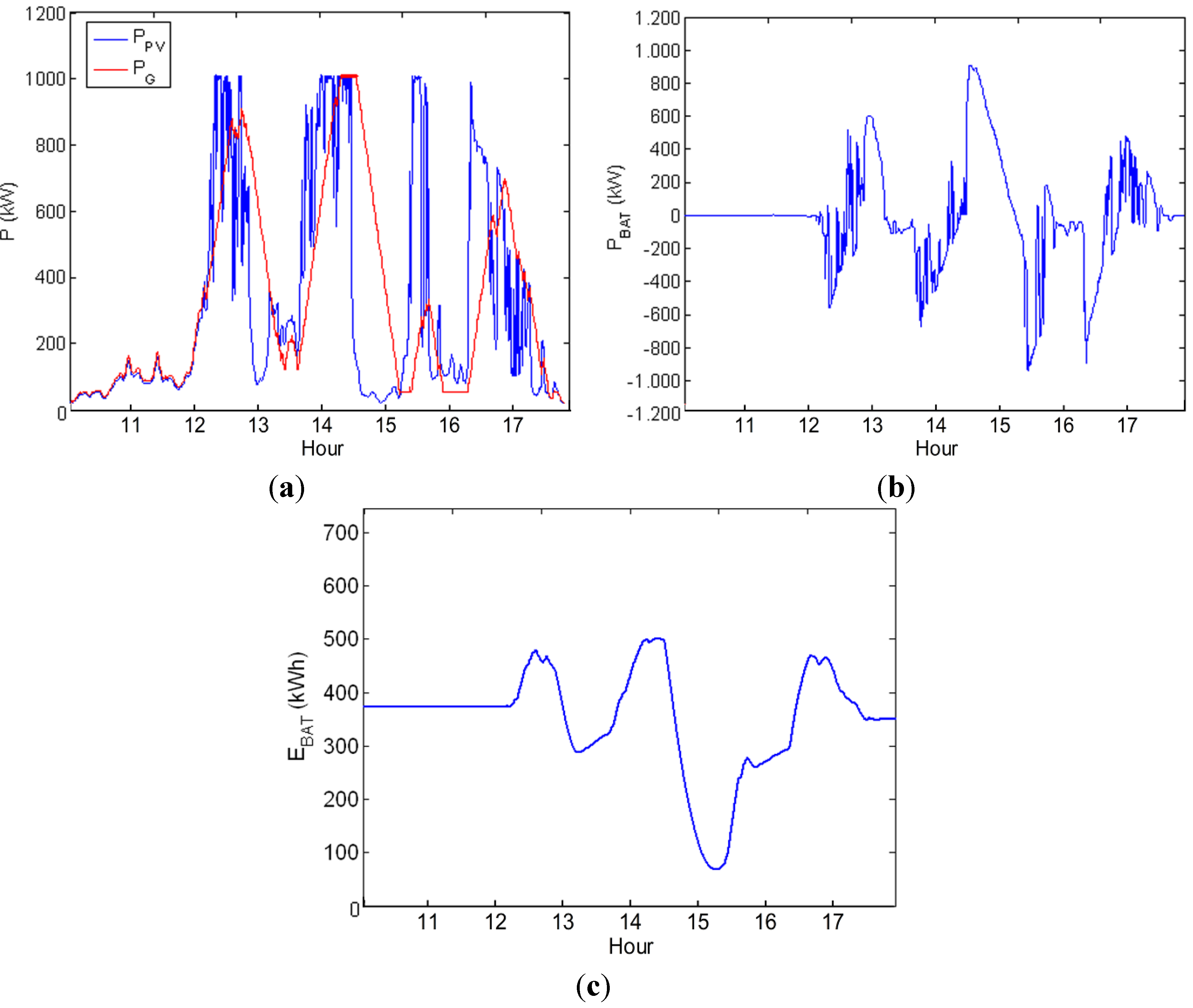
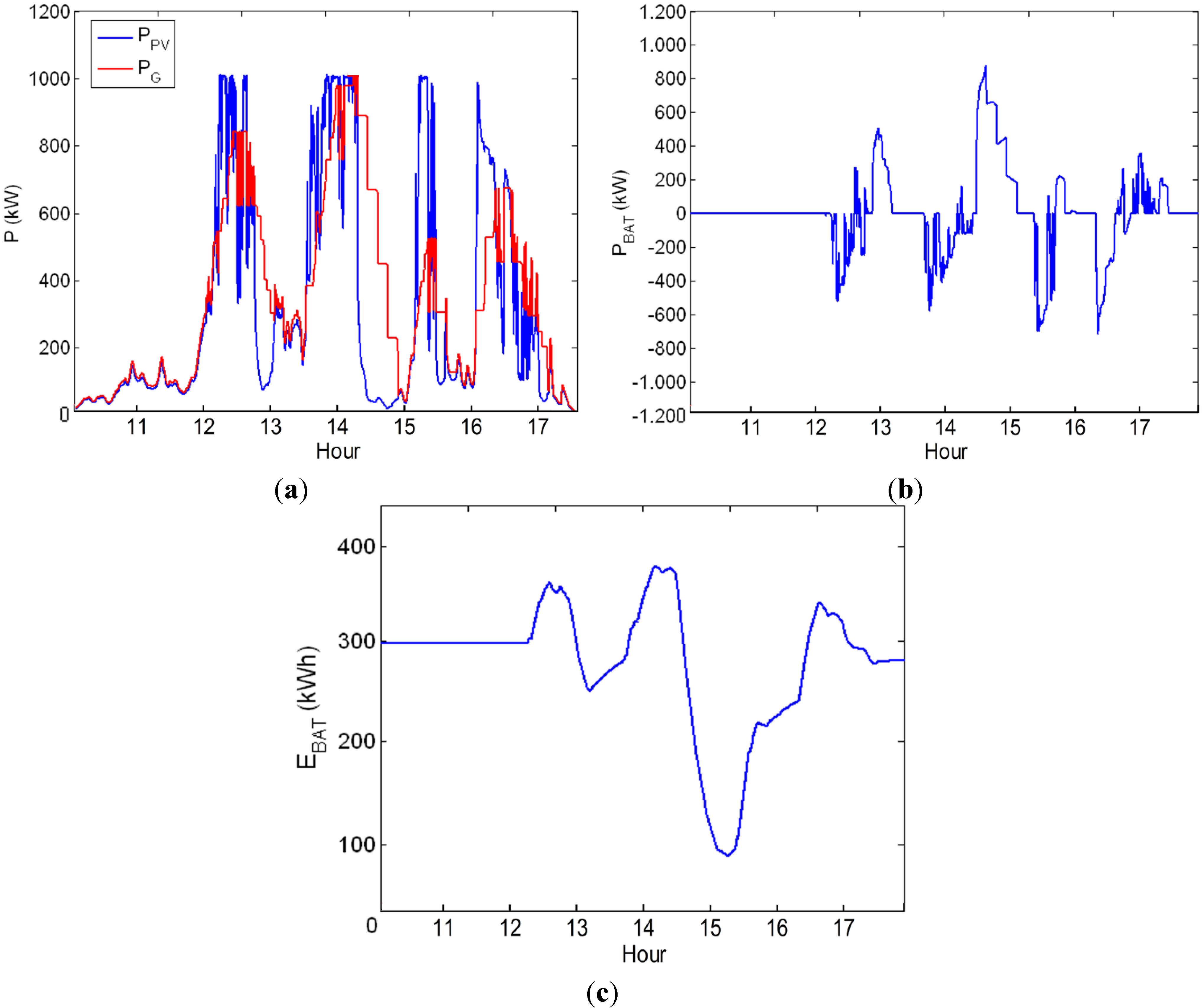
5. A Comparison of the Smoothing Strategies
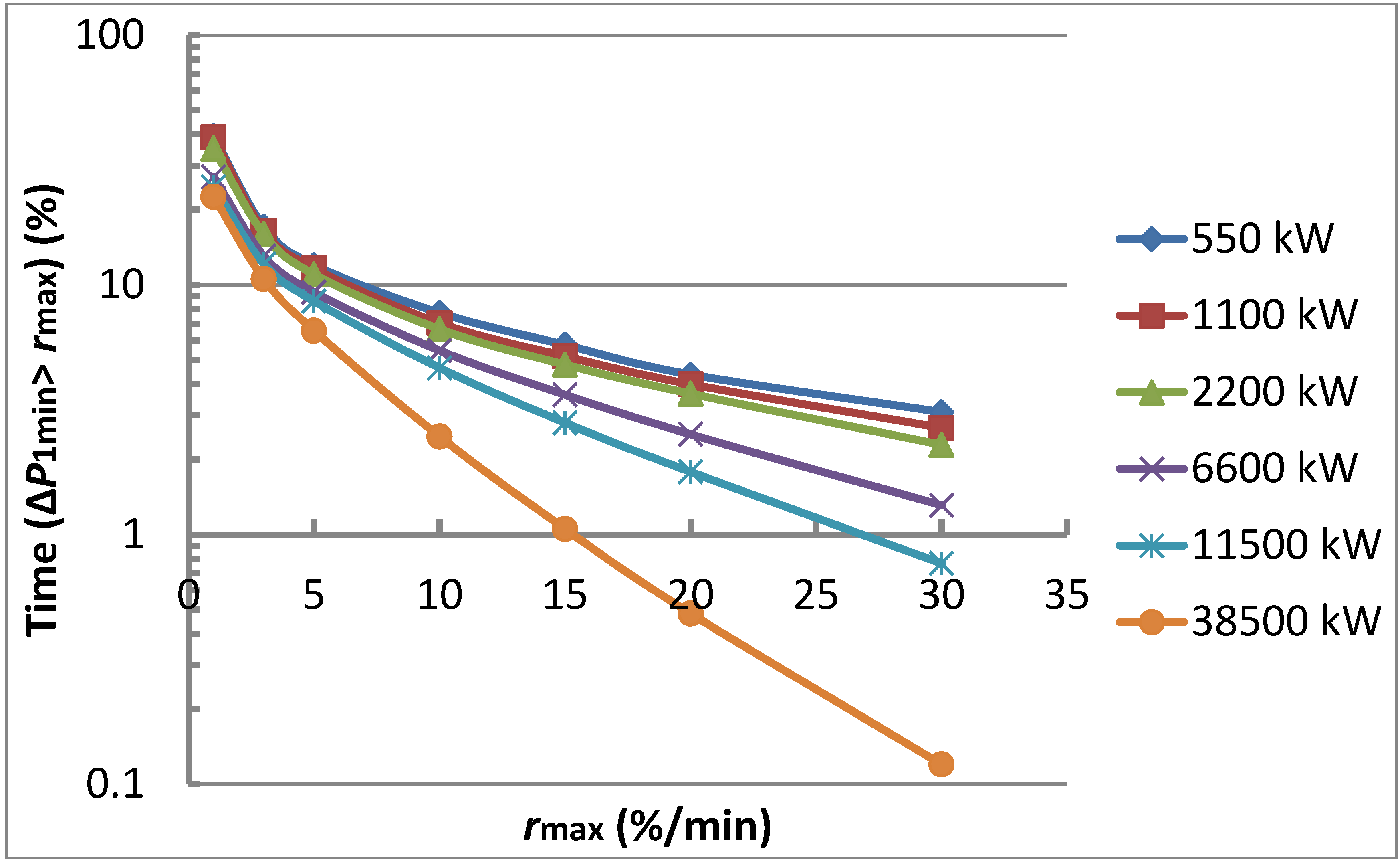
5.1. Effective Storage Time, tbat


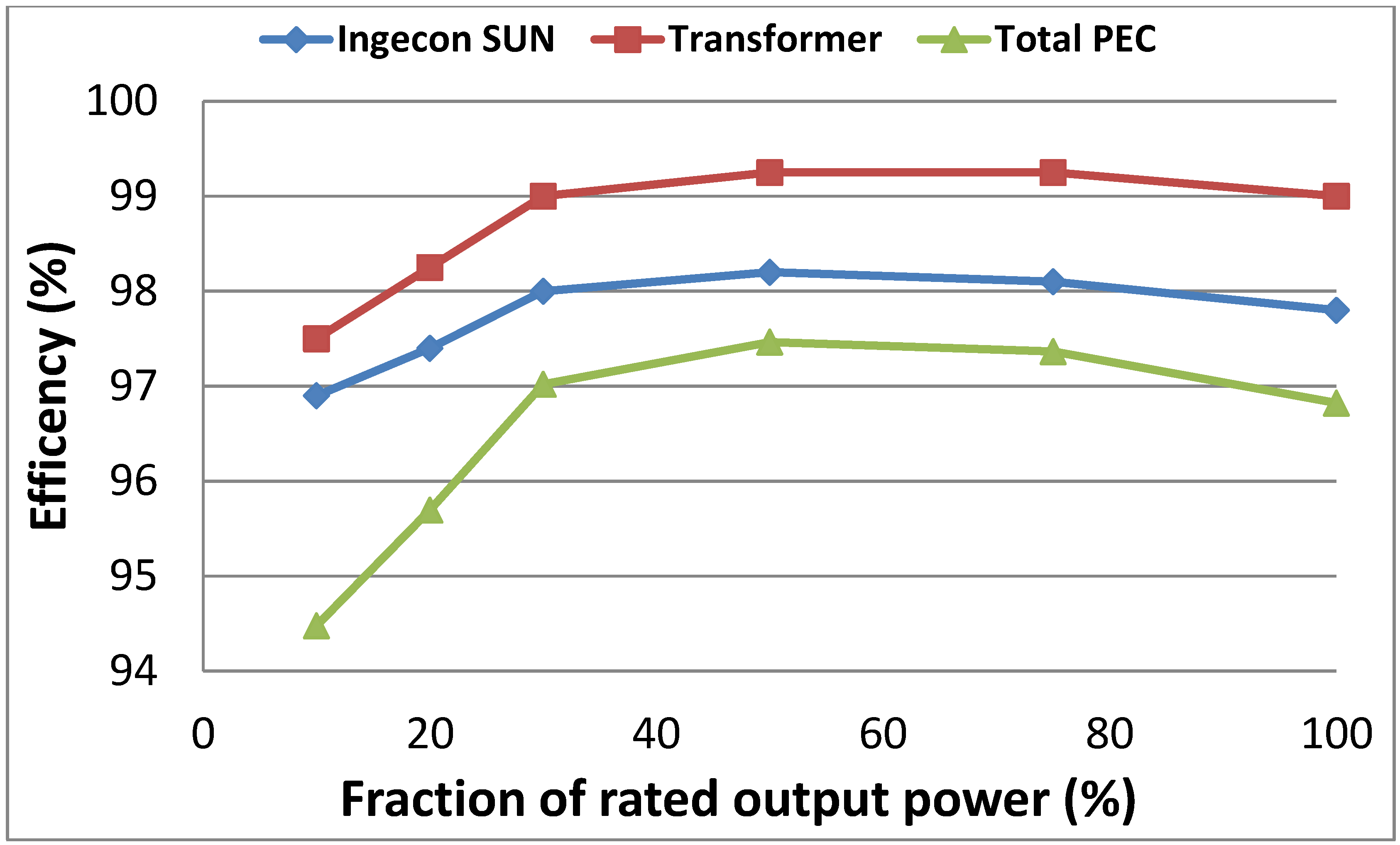
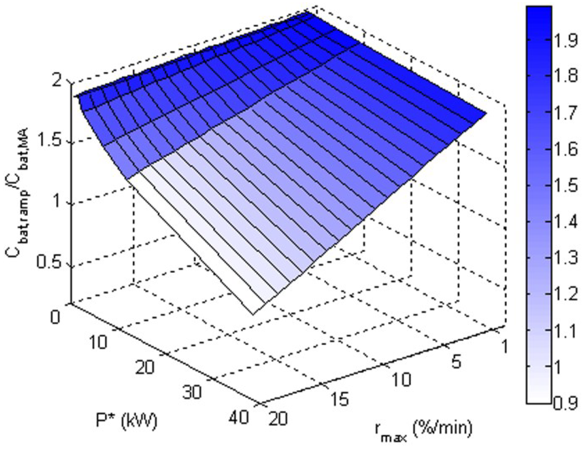
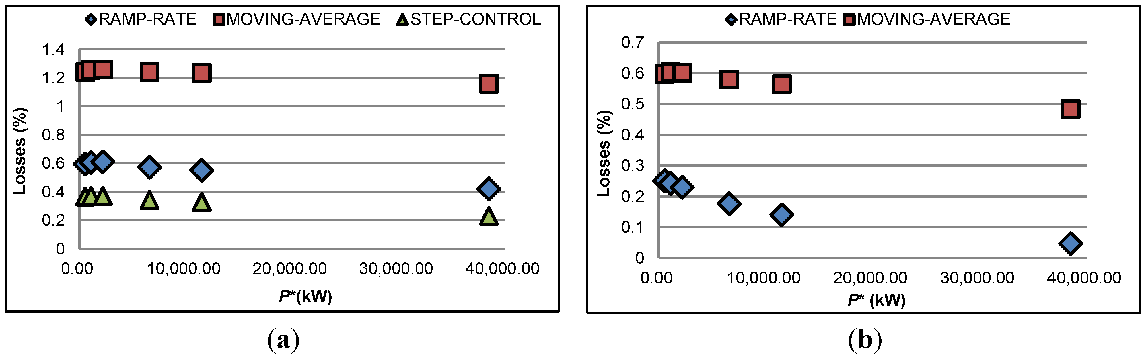
5.2. Losses in the Storage System

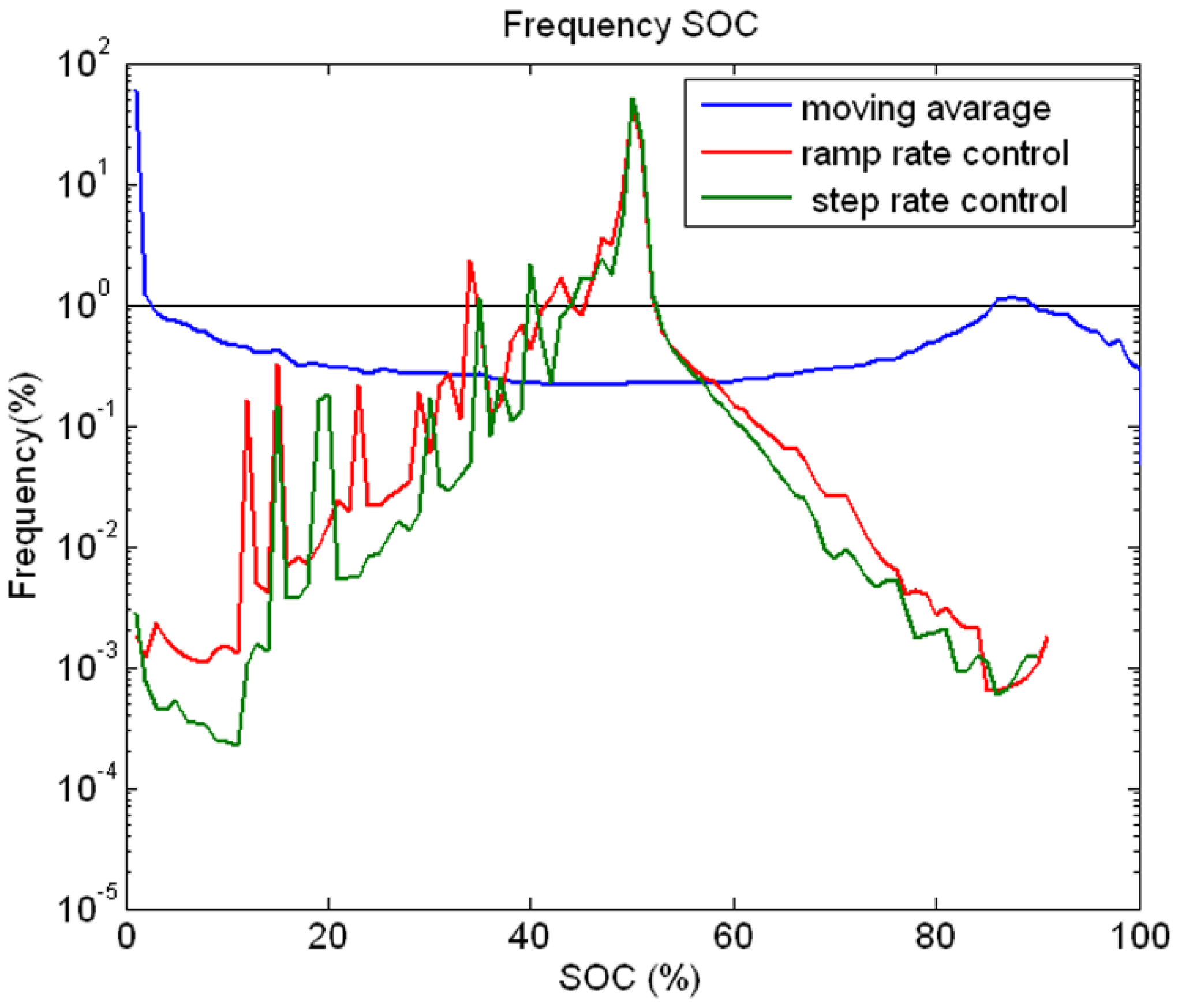
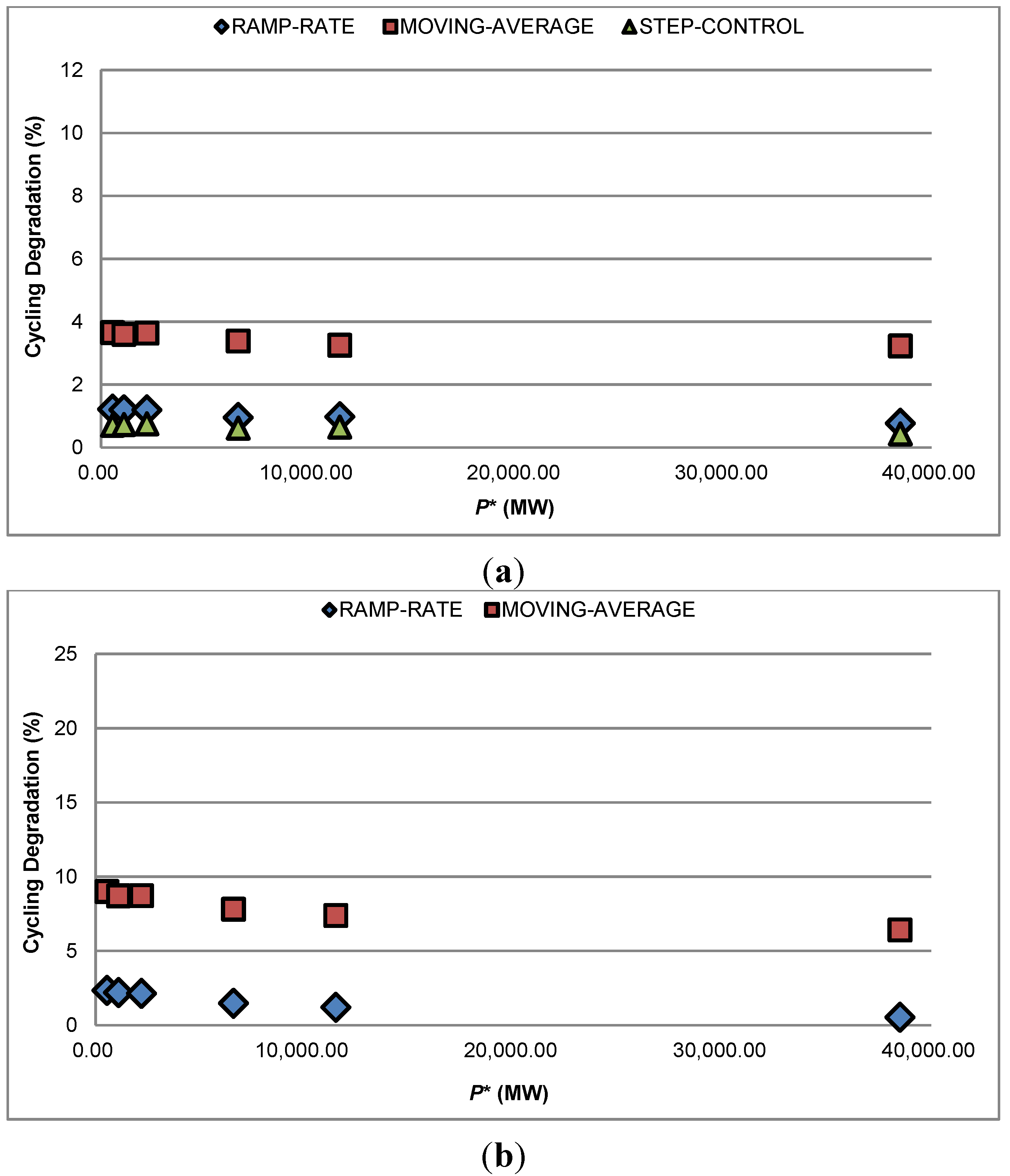
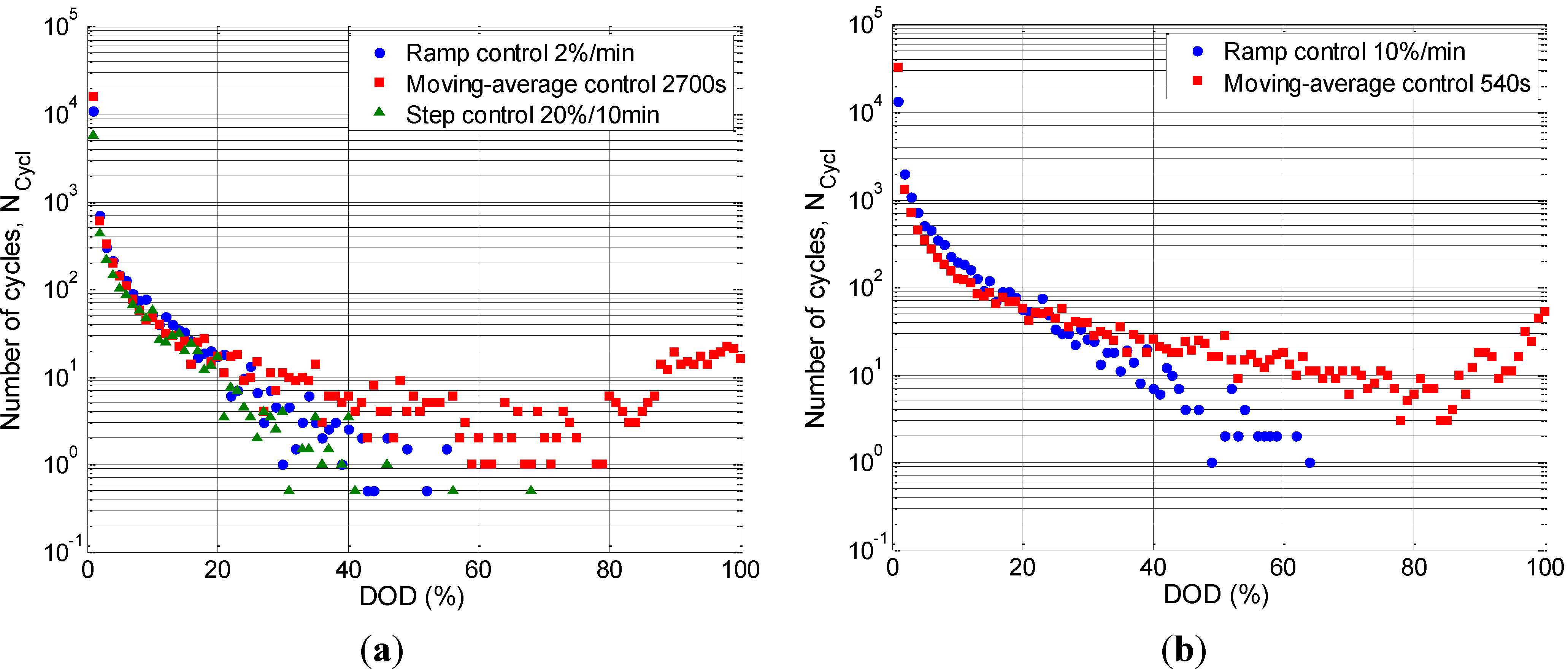
5.3. Stress in the Storage System


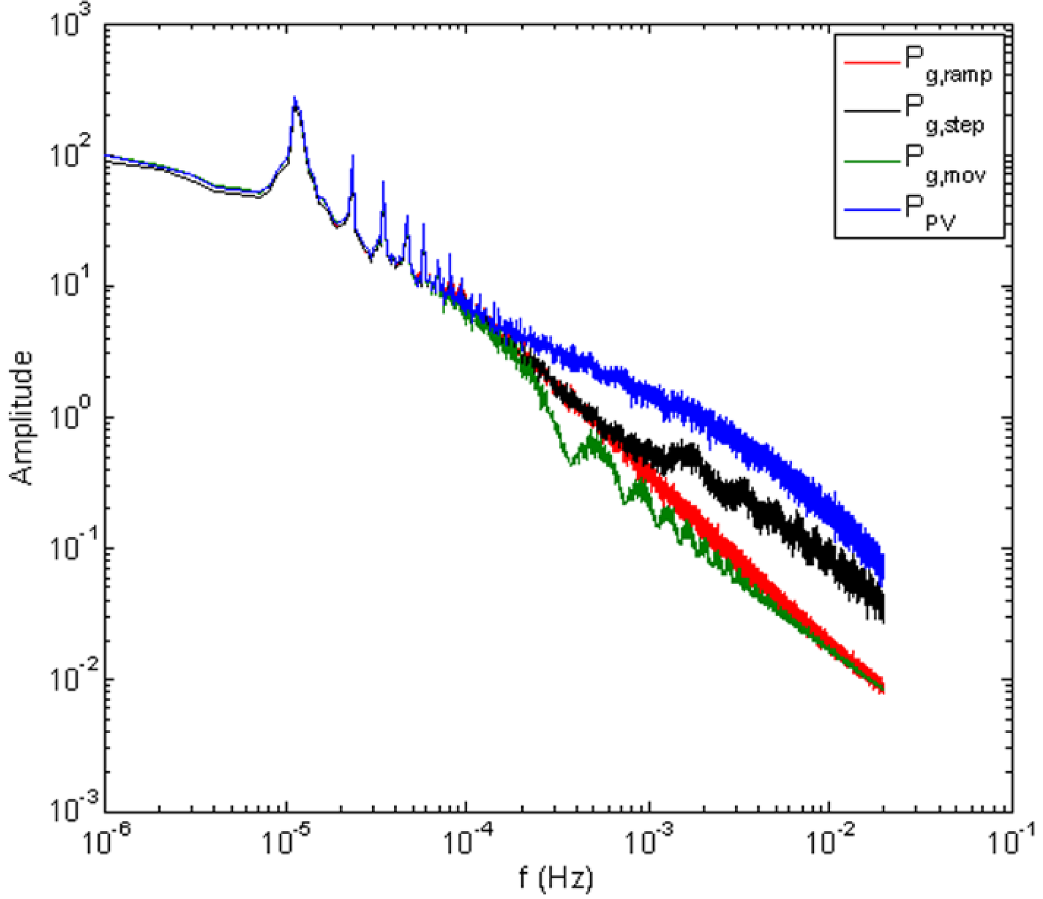
5.4. Quality of the Signal Injected into the Grid

6. Conclusions
Acknowledgments
Author Contributions
Conflicts of Interest
References
- PREPA Minimum Technical Requirements for Interconnection of Photovoltaic (PV) Facilities. Available online: http://www.fpsadvisorygroup.com/rso_request_for_quals/PREPA_Appendix_E_PV_Minimum_Technical_Requirements.pdf (accessed on 6 March 2013).
- CRE Reglas Generales de Interconexión al Sistema Eléctrico Nacional: Anexo 3: Requerimientos Técnicos para Interconexión de Centrales Solares Fotovoltaicas al Sistema Eléctrico Nacional. Available online: http://www.cre.gob.mx/documento/3025.pdf (accessed on 31 January 2014). (In Spanish)
- National Energy Regulator of South Africa (NERSA). Grid Connection Code for Renewable Power Plants (RPPs) Connected to the Electricity Transmission System (TS) or the Distribution System (DS) in South Africa. Available online: http://www.nersa.org.za/Admin/Document/Editor/file/Electricity/TechnicalStandards/South African Grid Code Requirements for Renewable Power Plants - Vesion 2 6.pdf (accessed on 31 January 2014).
- Kuszamaul, S.; Ellis, A.; Stein, J.; Johnson, L. Lanai high-density irradiance sensor network for characterizing solar resource variability of MW-scale PV system. In Proceedings of the 2010 35th IEEE Photovoltaic Specialists Conference (PVSC), Honolulu, HI, USA, 20–25 June 2010; pp. 000283–000288.
- Otani, K.; Minowa, J.; Kurokawa, K. Study on areal solar irradiance for analyzing areally-totalized PV systems. Sol. Energy Mater. Sol. Cells 1997, 47, 281–288. [Google Scholar]
- Woyte, A.; Belmans, R.; Nijs, J. Fluctuations in instantaneous clearness index: Analysis and statistics. Sol. Energy 2007, 81, 195–206. [Google Scholar] [CrossRef]
- Mills, A. Understanding Variability and Uncertainty of Photovoltaics for Integration with the Electric Power System; Lawrence Berkeley National Laboratory: Berkeley, CA, USA, 2010. [Google Scholar]
- Lave, M.; Kleissl, J.; Arias-Castro, E. High-frequency irradiance fluctuations and geographic smoothing. Sol. Energy 2012, 86, 2190–2199. [Google Scholar] [CrossRef]
- Perez, R.; Hoff, T.E.; Schlemmer, J. Short-term irradiance variability: Station pair correlation as a function of distance. In Proceeding of the American Solar Energy Society (ASES) Annual Conference, Raleigh, NC, USA, 17–20 May 2011.
- Wiemken, E.; Beyer, H.G.G.; Heydenreich, W.; Kiefer, K. Power characteristics of PV ensembles: Experiences from the combined power production of 100 grid connected PV systems distributed over the area of Germany. Sol. Energy 2001, 70, 513–518. [Google Scholar] [CrossRef]
- Curtright, A.; Apt, J. The character of power output from utility scale photovoltaic systems. Prog. Photovolt. Res. Appl. 2008, 16, 241–247. [Google Scholar] [CrossRef]
- Perpiñán, O.; Marcos, J.; Lorenzo, E. Electrical power fluctuations in a network of DC/AC inverters in a large PV plant: Relationship between correlation, distance and time scale. Sol. Energy 2013, 88, 227–241. [Google Scholar] [CrossRef]
- Mills, A.; Wiser, R. Implications of Wide-Area Geographic Diversity for Short-Term Variability of Solar Power; Lawrence Berkeley National Laboratory: Berkeley, CA, USA, 2010. [Google Scholar]
- Marcos, J.; Marroyo, L.; Lorenzo, E.; Alvira, D.; Izco, E.; Ingeniería, D. Power output fluctuations in large scale PV plants: One year observations with one second resolution and a derived analytic model. Prog. Photovolt. Res. Appl. 2011, 19, 218–227. [Google Scholar] [CrossRef] [Green Version]
- Marcos, J.; Storkël, O.; Marroyo, L.; Garcia, M.; Lorenzo, E. Storage requirements for PV power ramp-rate control. Sol. Energy 2014, 99, 28–35. [Google Scholar] [CrossRef]
- Kakimoto, N.; Satoh, H.; Takayama, S.; Nakamura, K. Ramp-rate control of photovoltaic generator with electric double-layer capacitor. IEEE Trans. Energy Convers. 2009, 24, 465–473. [Google Scholar] [CrossRef]
- Khanh, L.N.; Seo, J.-J.; Kim, Y.-S.; Won, D.-J. Power-management strategies for a grid-connected PV-FC hybrid system. IEEE Trans. Power Deliv. 2010, 25, 1874–1882. [Google Scholar] [CrossRef]
- Yan, R.; Saha, T.K. Power ramp rate control for grid connected photovoltaic system. In Proceedings of the 2010 IPEC Conference, Singapore, 27–29 October 2010; pp. 83–88.
- Wang, L.; Lin, Y.-H.; Wang, L. Random fluctuations on dynamic stability of a grid-connected photovoltaic array. In Proceedings of the 2001 IEEE Power Engineering Society Winter Meeting, Columbus, OH, USA, 28 January–1 February 2001; Volume 3, pp. 985–989.
- Li, X.; Hui, D.; Lai, X. Battery energy storage station (BESS)-based smoothing control of photovoltaic (PV) and wind power generation fluctuations. IEEE Trans. Sustain. Energy 2013, 4, 464–473. [Google Scholar] [CrossRef]
- Alam, M.; Muttaqi, K.; Sutanto, D. A novel approach for ramp-rate control of solar PV using energy storage to mitigate output fluctuations caused by cloud passing. IEEE Trans. Energy Convers. 2014, 29, 507–518. [Google Scholar] [CrossRef]
- Datta, M.; Senjyu, T.; Yona, A.; Funabashi, T.; Kim, C.-H. Photovoltaic output power fluctuations smoothing methods for single and multiple PV generators. Curr. Appl. Phys. 2010, 10, S265–S270. [Google Scholar] [CrossRef]
- Seo, H.-R.; Kim, G.-H.; Kim, S.-Y.; Kim, N.; Lee, H.-G.; Hwang, C.; Park, M.; Yu, I.-K. Power quality control strategy for grid-connected renewable energy sources using PV array and supercapacitor. In Proceedings of the 2010 International Conference on Electrical Machines and Systems (ICEMS), Incheon, Korea, 10–13 October 2010; pp. 437–441.
- Chanhom, P.; Sirisukprasert, S.; Hatti, N. A new mitigation strategy for photovoltaic power fluctuation using the hierarchical simple moving average. In Proceedings of the 2013 IEEE International Workshop on Intelligent Energy Systems (IWIES), Vienna, Austria, 14 November 2013; pp. 28–33.
- Han, X.; Chen, F.; Cui, X.; Li, Y.; Li, X. A power smoothing control strategy and optimized allocation of battery capacity based on hybrid storage energy technology. Energies 2012, 5, 1593–1612. [Google Scholar] [CrossRef]
- Beltran, H.; Bilbao, E.; Belenguer, E.; Etxeberria-Otadui, I.; Rodriguez, P. Evaluation of storage energy requirements for constant production in PV power plants. IEEE Trans. Ind. Electron. 2013, 60, 1225–1234. [Google Scholar] [CrossRef]
- Darras, C.; Muselli, M.; Poggi, P.; Voyant, C.; Hoguet, J.-C.; Montignac, F. PV output power fluctuations smoothing: The MYRTE platform experience. Int. J. Hydrog. Energy 2012, 37, 14015–14025. [Google Scholar] [CrossRef]
- Nuhic, A.; Terzimehic, T.; Soczka-Guth, T.; Buchholz, M.; Dietmayer, K. Health diagnosis and remaining useful life prognostics of lithium-ion batteries using data-driven methods. J. Power Sources 2013, 239, 680–688. [Google Scholar] [CrossRef]
- Beltran, H.; Swierczynski, M.; Luna, A.; Vazquez, G.; Belenguer, E. Photovoltaic plants generation improvement using Li-ion batteries as energy buffer. In Proceedings of the 2011 IEEE International Symposium on Industrial Electronics (ISIE), Gdansk, Poland, 27–30 June 2011; pp. 2063–2069.
- Cheng, F.; Willard, S.; Hawkins, J.; Arellano, B.; Lavrova, O.; Mammoli, A. Applying battery energy storage to enhance the benefits of photovoltaics. In Proceedings of the 2012 IEEE Energytech, Cleveland, OH, USA, 29–31 May 2012; pp. 1–5.
- Marcos, J.; Marroyo, L.; Lorenzo, E.; García, M. Smoothing of PV power fluctuations by geographical dispersion. Prog. Photovolt. Res. Appl. 2012, 20, 226–237. [Google Scholar] [CrossRef]
- Hoff, T.E.; Perez, R. Quantifying PV power output Variability. Sol. Energy 2010, 84, 1782–1793. [Google Scholar] [CrossRef]
- Ingeteam. INGECON SUN POWERMAX (275–1070 kW). Available online: http://www.ingeteam.com/es-es/energia/energia-fotovoltaica/p15_24_36/ingecon-sun-powermax.aspx (accessed on 14 October 2014).
- SAFT SA. Intensium® Flex, Product Brochure. 2008. Available online: http://www.saftbatteries.com/battery-search/intensium%C2%AE-flex (accessed on 31 January 2014).
- Downing, S.D.; Socie, D.F. Simple rainflow counting algorithms. Int. J. Fatigue 1982, 4, 31–40. [Google Scholar] [CrossRef]
- Hund, T.D.; Gonzalez, S.; Barrett, K. Grid-tied PV system energy smoothing. In Proceedings of the 2010 35th IEEE Photovoltaic Specialists Conference (PVSC), Honolulu, HI, USA, 20–25 June 2010; pp. 002762–002766.
- Matsuishi, M.; Endo, T. Fatigue of metals subjected to varying stress. Jpn. Soc. Mech. Eng. 1968, 96, 37–40. [Google Scholar]
- Dufo-López, R.; Bernal-Agustín, J.L.; Contreras, J. Optimization of control strategies for stand-alone renewable energy systems with hydrogen storage. Renew. Energy 2007, 32, 1102–1126. [Google Scholar] [CrossRef]
- Dufo-López, R.; Lujano-Rojas, J.M.; Bernal-Agustín, J.L. Comparison of different lead-acid battery lifetime prediction models for use in simulation of stand-alone photovoltaic systems. Appl. Energy 2014, 115, 242–253. [Google Scholar] [CrossRef]
- Datta, M.; Senjyu, T.; Yona, A.; Funabashi, T. Photovoltaic output power fluctuations smoothing by selecting optimal capacity of battery for a photovoltaic-diesel hybrid system. Electr. Power Compon. Syst. 2011, 39, 621–644. [Google Scholar] [CrossRef]
- Gee, A.M.; Robinson, F.V.P.; Dunn, R.W. Analysis of battery lifetime extension in a small-scale wind-energy system using supercapacitors. IEEE Trans. Energy Convers. 2013, 28, 24–33. [Google Scholar] [CrossRef]
- Schaltz, E.; Khaligh, A.; Rasmussen, P.O. Influence of battery/ultracapacitor energy-storage sizing on battery lifetime in a fuel cell hybrid electric vehicle. IEEE Trans. Veh. Technol. 2009, 58, 3882–3891. [Google Scholar] [CrossRef]
- Perez, R.; Kivalov, S.; Hoff, T.E.; Dise, J.; Chalmers, D. Mitigating short-term PV output intermittency. In Proceedings of the 28th European Photovoltaic Solar Energy Conference and Exhibition (EU PVSEC), Villepinte, France, 30 September–4 October 2013; pp. 3719–3726.
- Marcos, J.; Marroyo, L.; Lorenzo, E.; Alvira, D.; Izco, E. From irradiance to output power fluctuations: The PV plant as a low pass filter. Prog. Photovolt. Res. Appl. 2011, 19, 505–510. [Google Scholar] [CrossRef] [Green Version]
- Apt, J. The spectrum of power from wind turbines. J. Power Sources 2007, 169, 369–374. [Google Scholar] [CrossRef]
© 2014 by the authors; licensee MDPI, Basel, Switzerland. This article is an open access article distributed under the terms and conditions of the Creative Commons Attribution license (http://creativecommons.org/licenses/by/4.0/).
Share and Cite
Marcos, J.; De la Parra, I.; García, M.; Marroyo, L. Control Strategies to Smooth Short-Term Power Fluctuations in Large Photovoltaic Plants Using Battery Storage Systems. Energies 2014, 7, 6593-6619. https://doi.org/10.3390/en7106593
Marcos J, De la Parra I, García M, Marroyo L. Control Strategies to Smooth Short-Term Power Fluctuations in Large Photovoltaic Plants Using Battery Storage Systems. Energies. 2014; 7(10):6593-6619. https://doi.org/10.3390/en7106593
Chicago/Turabian StyleMarcos, Javier, Iñigo De la Parra, Miguel García, and Luis Marroyo. 2014. "Control Strategies to Smooth Short-Term Power Fluctuations in Large Photovoltaic Plants Using Battery Storage Systems" Energies 7, no. 10: 6593-6619. https://doi.org/10.3390/en7106593