Simplified Analysis of the Electric Power Losses for On-Shore Wind Farms Considering Weibull Distribution Parameters

Abstract
:1. Introduction
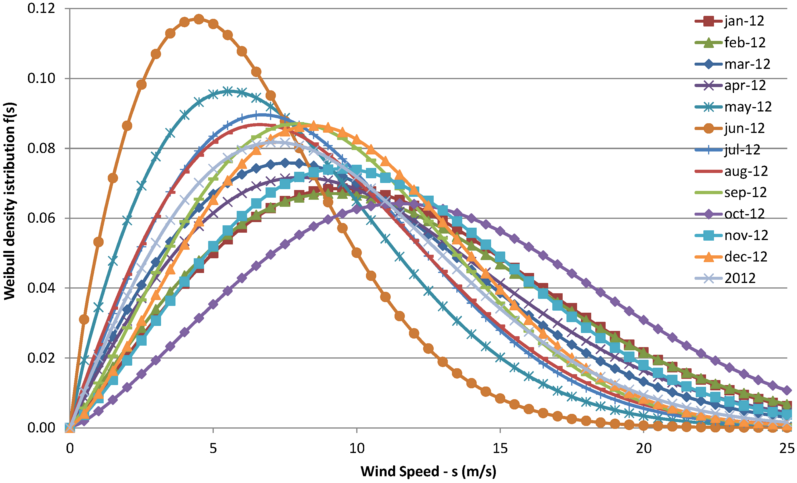
2. Characterization and Variability of the Wind Resource


| Weibull parameters | Period | ||||||||||||
|---|---|---|---|---|---|---|---|---|---|---|---|---|---|
| Jan. | Feb. | Mar. | Apr. | May | Jun. | Jul. | Aug. | Sep. | Oct. | Nov. | Dec. | Year | |
| Shape—k | 2.09 | 2.02 | 1.94 | 1.93 | 1.85 | 1.81 | 1.99 | 1.93 | 2.19 | 2.30 | 2.21 | 2.28 | 1.96 |
| Scale—λ (m/s) | 12.92 | 12.86 | 11.09 | 11.72 | 8.50 | 6.90 | 9.54 | 9.67 | 10.48 | 14.73 | 12.40 | 10.89 | 10.35 |
| Mean wind speed | 11.44 | 11.39 | 9.83 | 10.39 | 7.54 | 6.14 | 8.45 | 8.57 | 9.28 | 13.05 | 10.98 | 9.64 | 9.17 |

3. Calculation of the Electrical Losses
3.1. Application to One WTG

3.1.1. Energy Losses

3.1.2. Energy Generated
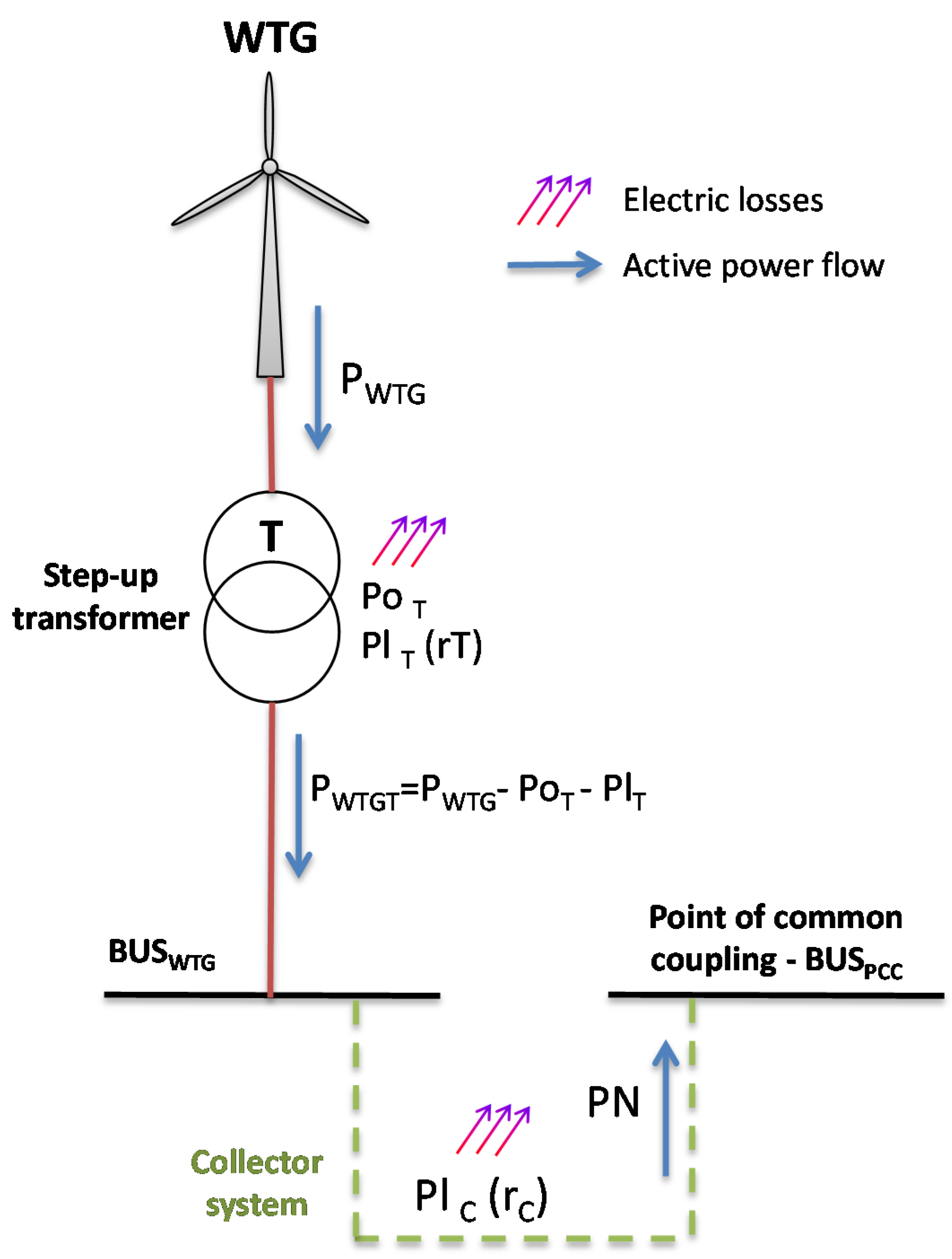
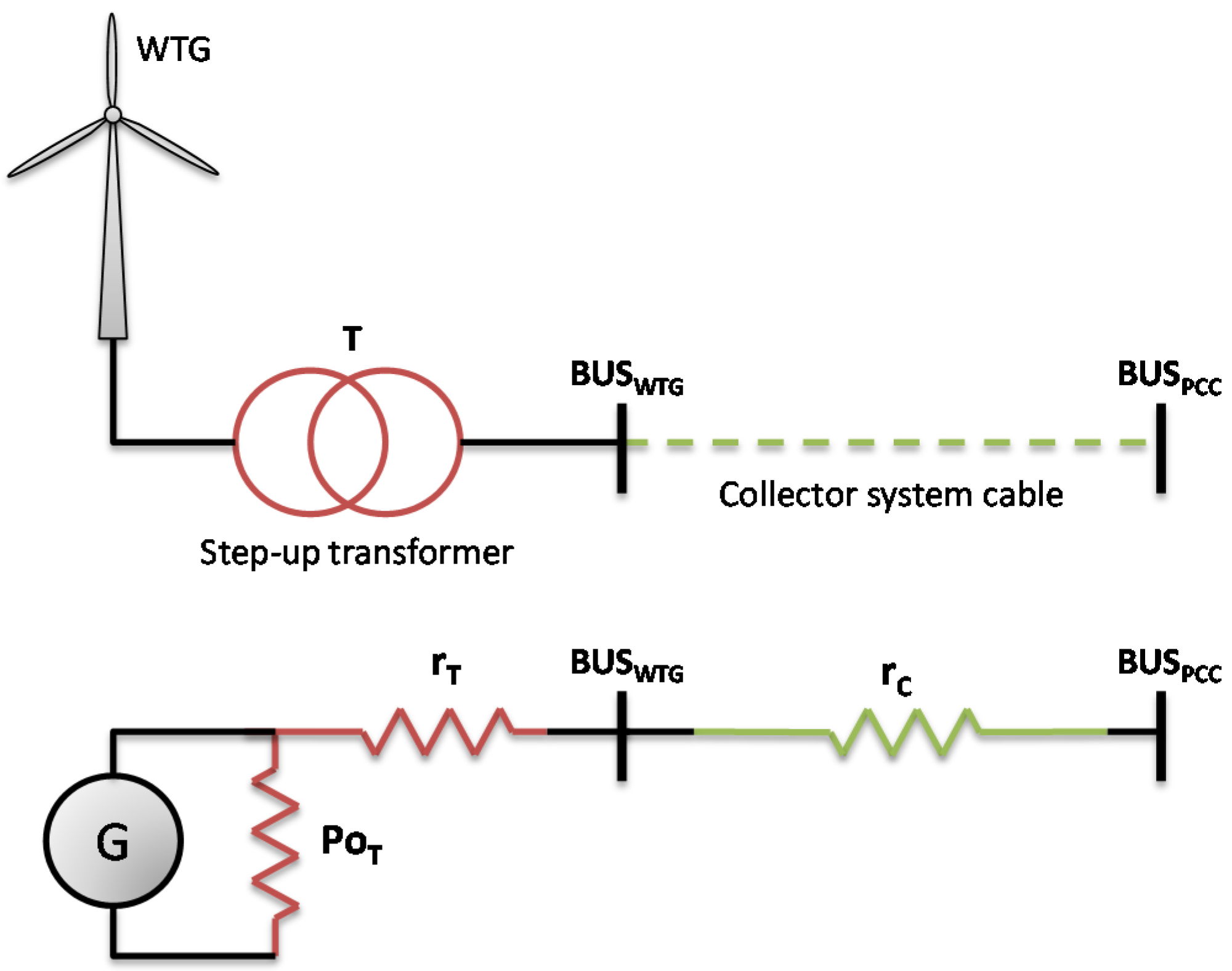
3.1.3. Characterization of the Electrical Infrastructures
- The WTG as an ideal generator of which instantaneous power output is obtained from the power curve corresponding with the wind speed at the hub height. This representation does not introduce error in the calculations because the power curve gives the net power output for all the wide range of operating voltage of the WTG.
- The WTG step-up transformer by means of a parallel resistance for the non-load losses and a serial resistance for the load losses.
- The collector system cable between the BUSWTG and the BUSPCC with a serial resistance .

| Element | Name | Value | Unit | Comment |
|---|---|---|---|---|
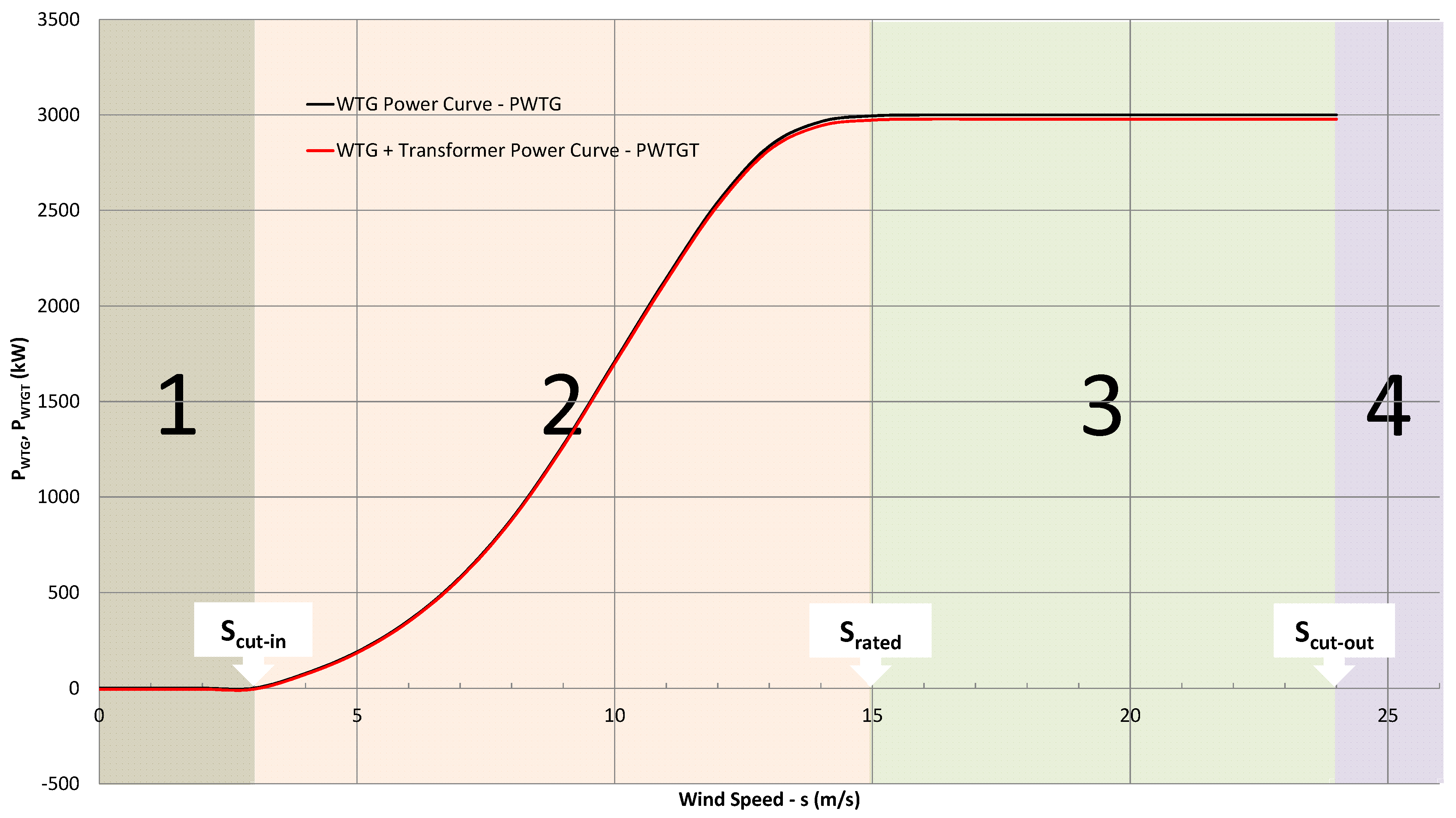
| WTG | Manufacturer and type | Vestas V112-3 MW | – | Class I WTG [40] 112 m of rotor diameter |
| Power curve | Figure 4 | – | Vestas standard | |
| Step-up transformer | Manufacturer and type | Standard for V112-3 MW | – | – |
| PoT | 5.3 | kW | Manufacturer data for the WTG selected | |
| rT | 2.42 | Ω | Manufacturer data for the WTG selected. Corresponds with a 0.7% of positive sequence short-circuit resistance at the transformer rated power | |
| Collector system | VGRID | 36 | kV | Typical |
| Interconnection cable to the collector system | Length (L) | 350 | m | The selected WTG has a 112 m rotor diameter. To reduce weak losses the separation between neighbour WTGs should be in the range of 2 or 3 times the length of the rotor diameter |
| Material | Al | Typical | ||
| Size | 120 | mm2 | Medium value | |
| Insulation material | XLPE/EPR | Typical | ||
| rC per km | 0.3226 | Ω/km | – | |
| rC | 0.1129 | Ω | – |
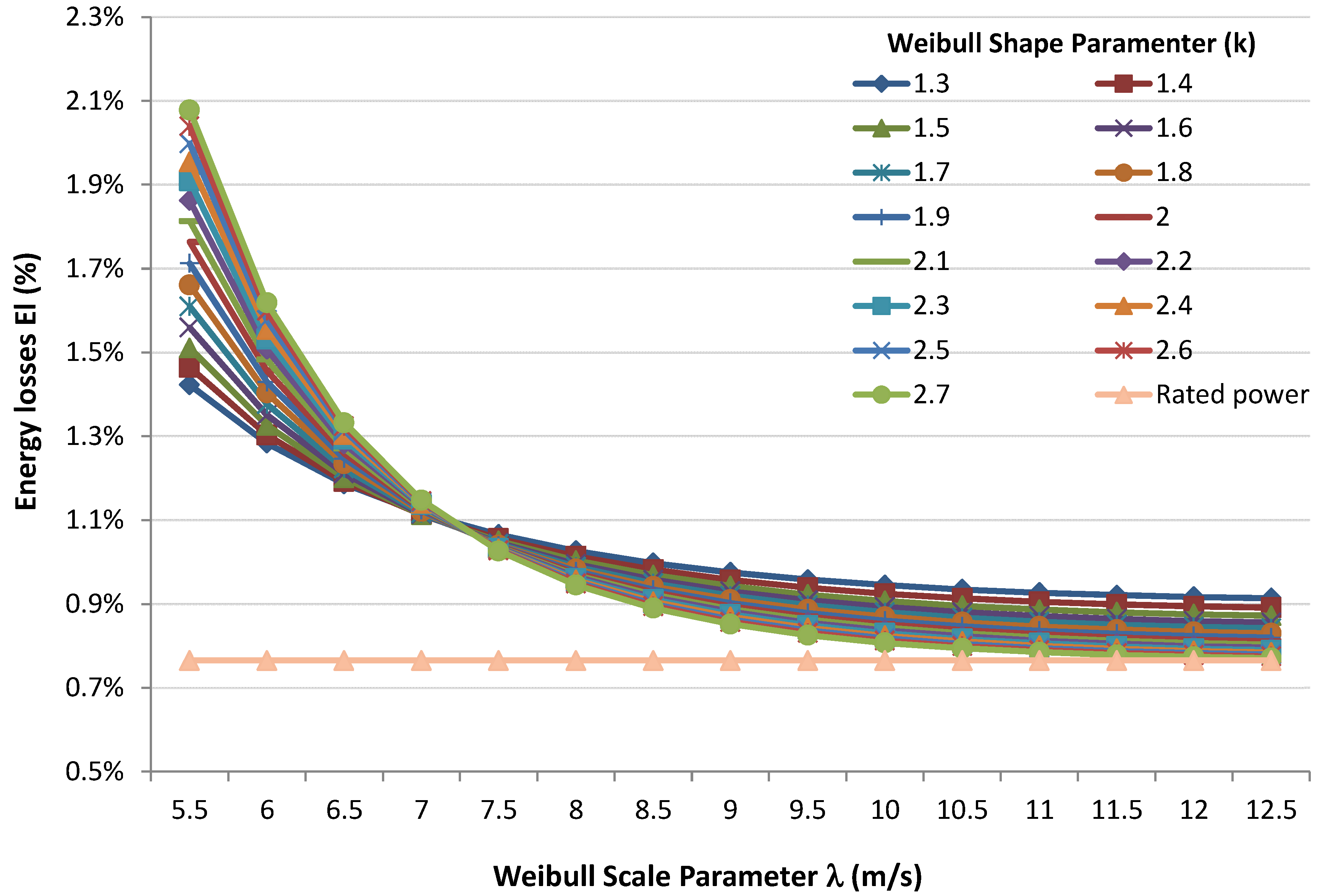
3.1.4. Calculation and Simulation Results

3.2. Application to a WF

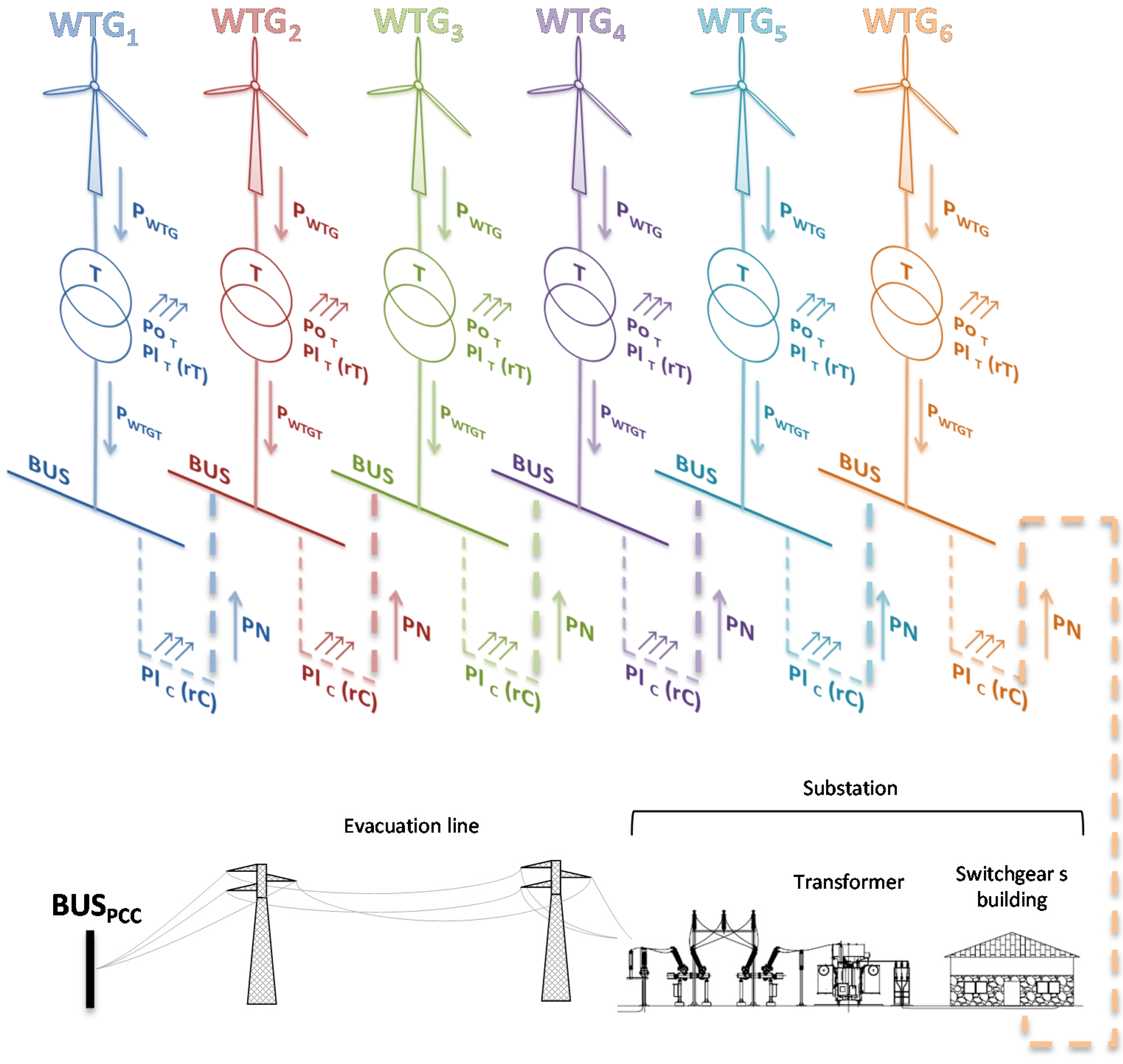
3.2.1. Energy Losses
- The active power generated by the WTG, , reduced by the losses of the step-up transformer .
- The addition of the net active power coming from the previous bus, .
- The subtraction of the electric losses in the cable between both cables, .


3.2.2. Energy Generated
3.2.3. Characterization of the WF and the Electric Infrastructures
- The substation transformer by means of a parallel resistance for the non-load losses and a serial resistance for the load losses. Both parameters are obtained from the standard short-circuit and losses test carried out for every single transformer.
- The evacuation line between the substation (BUSST) and the BUSPCC with a serial resistance .
- The evacuation voltage magnitude is, in general, different and higher than the collector system voltage magnitude.
| Voltage (kV) | 147-AL1/34-ST1A a | 242-AL1/39-ST1A | 402-AL1/52-ST1A |
|---|---|---|---|
| Power limit (cos φ = 0.8) (MVA) | |||
| 45 | 26.95 | 36.11 | 50.38 |
| 66 | 39.53 | 52.96 | 73.89 |
| 132 | 79.05 | 105.91 | 147.79 |
| 220 | Not used | Not used | 246.31 |
| – | 147-AL1/34-ST1A | 242-AL1/39-ST1A | 402-AL1/52-ST1A |
| – | Resistance at 85 °C | ||
| rCL (Ω/km) | 0.2483 | 0.1195 | 0.0719 |
| Element | Name | Value | Unit | Comment |
|---|---|---|---|---|
| Wind Farm | Power | 54 | MW | 18 × 3 MW |
| Composition | 3 circuits 6 WTG per circuit | – | – | |
| Substation transformer | Nominal Power | 60 | MVA | – |
| PoST | 40 | kW | Manufacturer data | |
| Ucc | 11.00 | % | According to standard IEC 60076 [50] | |
| – | x/r | 35 | – | IEEE Transformers Committee recommendations [51] |
| PCC Voltage | VGRID | 132 | kV | Typical |
| Evacuation line | Length (L) | 15 | km | – |
| Material | 147-AL1/34-ST1A | – | Designation according to standard UNE-EN 50 182 (Spanish standard equivalent to IEC 61089). See Table 3 | |
| rCL per km | 3.7251 | Ω/km | Value for the cable selected. Source [49] |
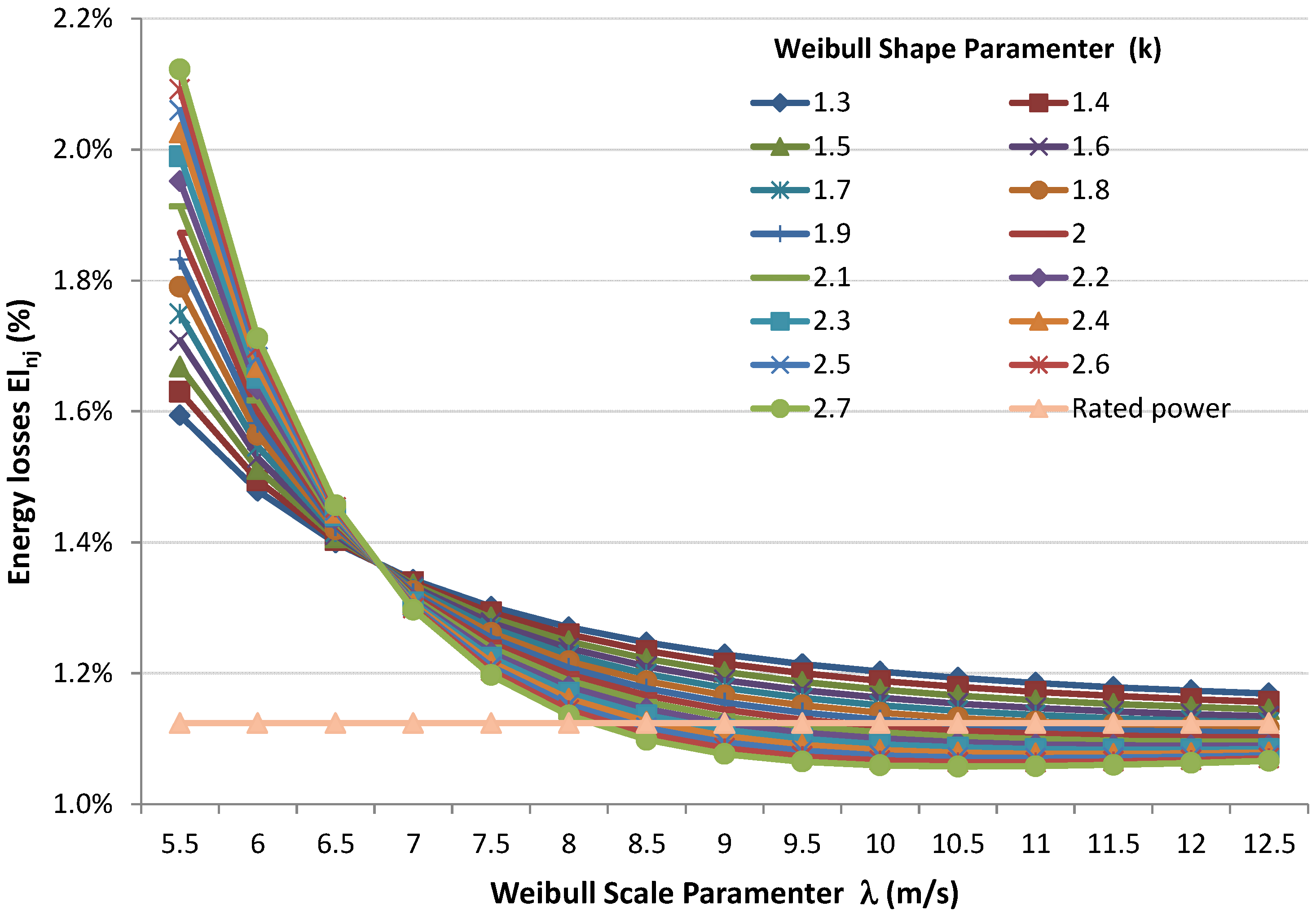
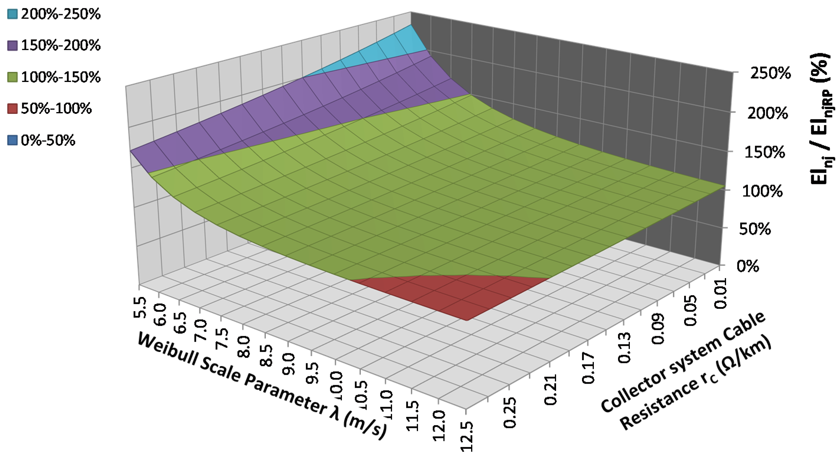
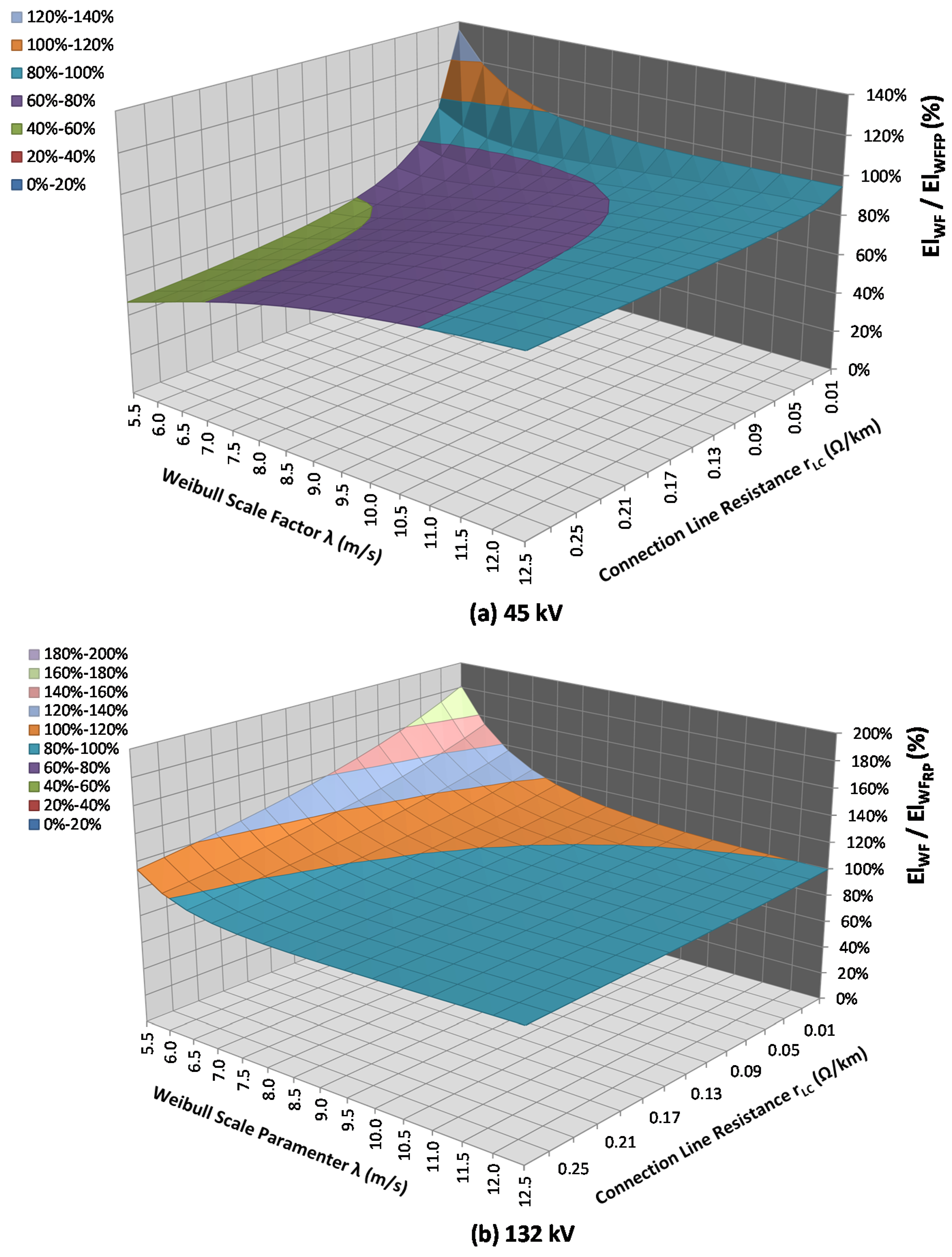
3.2.4. Simulation Results and Sensitivity Analysis


3.3. Comparative of the Behaviour of the Electric Losses
3.4. Validity of the Proposed Method
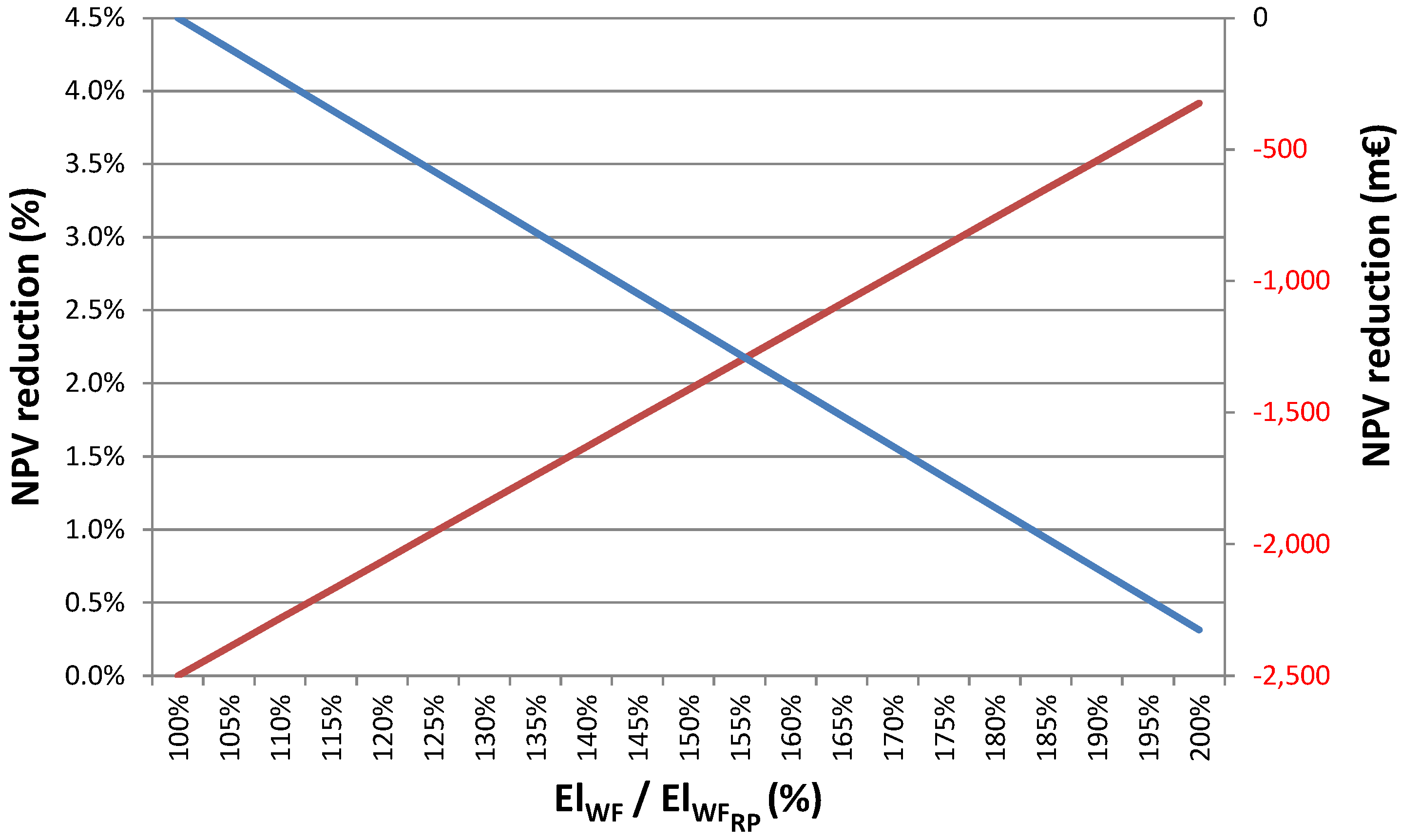
4. Impact of the Losses in the Financial Value of the WF
| Cash Flow | |
|---|---|
| + | Incomes from electricity remuneration |
| − | Operating expenses |
| = | Gross operating margin (EBITDA) |
| − | Depreciation |
| = | Earnings before interests and taxes (EBIT) |
| − | Financial expenses |
| = | Earnings before taxes |
| − | Taxes |
| = | Earnings after taxes |
| + | Depreciation |
| = | Yearly cash flow (CFz) |
| Breakdown | Name | Value | Unit | Comment |
|---|---|---|---|---|
| Prices | Wind Farm Construction | 1,100 | €/kW | Sources [13,30,53,54] |
| 20.00 | €/MWh | Source [8,53] | ||
| Land easements | 3,000 | €/(MW × year) | Includes assembly areas | |
| Insurance | 0.50 | % Incomes | All risk and Civil Liability. Typically calculated over incomes | |
| Administration | 0.02 | % Incomes | Typically calculated over incomes | |
| Yearly prices increase | 2 | % | Typically indexed to inflation. Estimate based on the trend in the inflation forecast [55,56] | |
| Power purchase agreement | Initial PPA price | 80.00 | €/MWh | Estimated from [10] |
| Yearly increase | 2 | % | Typically indexed to inflation. Estimate based on the trend in the inflation forecast [55,56] | |
| Electricity generation | Gross capacity factor | 30 | % | – |
| Wake losses | 5 | % | – | |
| Losses factor | 1 | % | Includes up to grid connection point | |
| WTG Mechanical Availability | 97 | % | WTG Mechanical availability is defined typically in a yearly period, as the percentage of time (year) in which the WTG is ready to roduce electricity Current market value. Source: WTG Manufacturers | |
| Taxes | Profit taxes | 30 | % | – |
| Income taxes | 2 | % | The final value depends on council and the incomes level. Mean value has been taken into consideration | |
| Financial terms | Depreciation period | 10 | years | Typical |

5. Conclusions
Nomenclature
Weibull distribution
| f(s) | Probability density function for the wind speed Weibull distribution |
| λ | Scale parameter of the Weibull distribution (m/s) |
| k | Shape parameter of the Weibull distribution |
| F(s) | Cumulative distribution function for the wind speed Weibull distribution. |
| (s) | Wind speed (m/s) |
Wind turbine and wind farm characteristics
| BUSPCC | Point of common coupling bus |
| BUSST | Bus of connection to all the collector system circuits with the evacuation line. Represents the wind farm substation. |
| BUSWTG | Bus in which the wind turbine is connected to the collector system. |
| nC | Number of electric circuits in the wind farm |
| nWF | Number of wind turbines in the wind farm |
| PCC | Point of common coupling |
| rC | Resistance of the interconnection cable to the collector system |
| rCL | Resistance of the interconnection line |
| rST | Resistance representative of load active power losses in the substation transformer |
| rT | Resistance representative of load active power losses in the internal wind turbine step-up transformer |
| VPCC | Voltage magnitude in the point of common coupling |
| VGRID | Voltage magnitude of the collector system |
| WF | Wind Farm |
| WTG | Wind turbine generator |
Power flow analysis
| bpij | Parallel susceptance between buses i and j |
| Bij | Serial susceptance between buses i and j |
| Gij | Serial conductance between buses i and j |
| Pij | Active power flow from bus i to bus j |
| Qij | Reactive power flow from bus i to bus j |
| Vi | Voltage magnitude in the bus i. |
Admittance between buses i and j. | |
| θij | Difference between the voltage angles in buses i and j. |
Financial
| NPV | Net present value |
| CFz | Project cash flow in the year z |
| z | Ordinal indicating the number of years the PV system has been in service. |
| I | Investment value |
| r | Discount rate for NPV calculation |
Wind turbine generator power curve
| a, b, c | Coefficients of the polynom power curve adjust |
| PWTG | Power output of the wind turbine |
| PWTGT | Power output of the wind turbine minus the electric losses in the step-up transformer |
| Prated | Rated power of the wind turbine |
| Scut−in | Minimum wind speed at which the wind turbine will generate usable power |
| Scut−out | Wind speed at which wind turbine cease power generation and shut down |
| Srated | Minimum wind speed at which the wind turbine produces the rated power |
Energy and power flow
| CF | Capacity factor |
| Eg | Electricity generated by a wind turbine in the period T |
| EgWF | Electricity generated by the entire wind farm |
| El | Electricity losses in the period T |
| ElRP | Electricity losses when the wind turbine operates at rated power |
| Elnj | Energy losses in the circuit nj |
| ElnjRP | Energy losses in the circuit nj when all the wind turbines in the circuit operate at rated power |
| ElWF | Energy losses for the entire wind farm |
| ElWFRP | Energy losses for the entire wind farm when all the wind turbines operate at rated power |
| PGWF | Active power generated |
| Pl | Active power losses |
| PlC | Active power losses in the collector system cable |
| Plo | Active power losses when the wind turbine is not generating power |
| Plrated | Active power losses when the wind turbine operates at rated power |
| PlT | Load active power losses in the internal wind turbine step-up transformer |
| PlWF | Active power losses for the entire wind farm |
| PNANY | Net active power injected in the bus indicated (any) |
| PoST | No-load active power losses in the substation transformer |
| PoT | No-load active power losses in the internal wind turbine step-up transformer |
| T | Period of time for energy calculations |
Appendix A: Solution for the Integral
Author Contributions
Conflicts of Interest
References
- Díaz-Dorado, E.; Carrillo, C.; Cidrás, J.; Albo, E. Estimation of Energy Losses in a Wind Park. In Proceedings of the 9th International Conference Electrical Power Quality and Utilisation, Barcelona, Spain, 9–11 October 2007.
- González, J.S.; Gonzalez Rodriguez, A.G.; Mora, J.C.; Santos, J.R.; Payan, M.B. Optimization of wind farm turbines layout using an evolutive algorithm. Renew. Energy 2010, 35, 1671–1681. [Google Scholar]
- Inaba, N.; Takahashi, R.; Tamura, J.; Kimura, M.; Komura, A.; Takeda, K. A Consideration on Loss Characteristics and Annual Capacity Factor of Offshore Wind Farm. In Proceedings of the 2012 XXth International Conference on Electrical Machines (ICEM), Marseille, France, 2–5 September 2012; IEEE: New York, NY, USA, 2012; pp. 2022–2027. [Google Scholar]
- Takahashi, R.; Ichita, H.; Tamura, J.; Kimura, M.; Ichinose, M.; Futami, M.; Ide, K. Efficiency Calculation of Wind Turbine Generation System with Doubly-Fed Induction Generator. In Proceedings of the 2012 XXth International Conference on Electrical Machines (ICEM), Rome, Italy, 6–8 September 2010; IEEE: New York, NY, USA, 2010; pp. 1–4. [Google Scholar]
- Camm, E.H.; Behnke, M.R.; Bolado, O.; Bollen, M.; Bradt, M.; Brooks, C.; Dilling, W.; Edds, M.; Hejdak, W.J.; Houseman, D.; et al. Wind Power Plant Collector System Design Considerations: IEEE PES Wind Plant Collector System Design Working Group. In Proceedings of the 2009. PES '09. IEEE Power & Energy Society General Meeting, Calgary, AB, Canada, 26–30 July 2009; IEEE: New York, NY, USA, 2010; pp. 1–7. [Google Scholar]
- Camm, E.H.; Behnke, M.R.; Bolado, O.; Bollen, M.; Bradt, M.; Brooks, C.; Dilling, W.; Edds, M.; Hejdak, W.J.; Houseman, D.; et al. Wind Power Plant Substation and Collector System Redundancy, Reliability, and Economics. In Proceedings of the 2009. PES '09. IEEE Power & Energy Society General Meeting ; Power & Energy Society General Meeting, Calgary, AB, Canada, 26–30 July 2009; IEEE: New York, NY, USA, 2010; pp. 1–6. [Google Scholar]
- Steimer, P.K.; Apeldoorn, O. Medium voltage power conversion technology for efficient windpark power collection grids. In Proceedings of the 2010 2nd IEEE International Symposium on Power Electronics for Distributed Generation Systems (PEDG), Hefei, China, 16–18 June 2010; IEEE: New York, NY, USA, 2010; pp. 12–18. [Google Scholar]
- Blanco, M.I. The economics of wind energy. Renew. Sustain. Energy Rev. 2009, 13, 1372–1382. [Google Scholar] [CrossRef]
- The European Wind Energy Association. Wind in Power 2013. Available online: http://www.ewea.org/fileadmin/files/library/publications/statistics/EWEA_Annual_Statistics_2013.pdf (accessed on 21 September 2014).
- Asociación Empresarial Eólica. Eólica 2014; Asociación Empresarial Eólica: Madrid, Spain, 2014. (In Spanish) [Google Scholar]
- U.S. Department of Energy. Wind Technologies Market Report 2012; U.S. Department of Energy: Oak Ridge, TN, USA, 2013.
- Kalamova, M.; Kaminker, C.; Johnstone, N. Source of Finance, Investment Policies and Plant Entry in the Renewable Energy Sector; OECD Publishing: Paris, France, 2011. [Google Scholar]
- U.S. Department of Energy. Wind Technologies Market Report 2012; Lawrence Berkeley National Laboratory: Berkeley, CA, USA, 2013.
- Department of Energy Republic of South Africa Renewable Energy. Independent Power Producer Procurement Programme. Available online: http://www.ipprenewables.co.za/ (accessed on 25 June 2014).
- McGovern, M. Analysis—Uruguay, the next big South American market. In Wind Power Monthly; Haymarket Media Group Ltd.: London, UK, 2013. [Google Scholar]
- Carrillo, C.; Cidrás, J.; Díaz-Dorado, E.; Obando-Montaño, A.F. An Approach to Determine the Weibull Parameters for Wind Energy Analysis: The Case of Galicia (Spain). Energies 2014, 7, 2676–2700. [Google Scholar] [CrossRef]
- Villanueva, D.; Feijó, A.; Pazos, J.L. Multivariate Weibull distribution for wind speed and wind power behavior assessment. Resources 2013, 2, 370–384. [Google Scholar] [CrossRef]
- Amenedo Rodríguez, J.L.; Burgos Díaz, J.C.; Arnalte Gómez, S. Sistemas Eólicos de Producción de Energía Eléctrica; Rueda: Madrid, Spain, 2003; p. 439. (In Spanish) [Google Scholar]
- Carta González, J.A.; Calero Pérez, R.; Colmenar Santos, A.; Castro Gil, M.-A. Centrales de Energías Renovables: Generación Eléctrica con Energías Renovables; Pearson Educación ,S.A.: Madrid, Spain, 2009; p. 703. (In Spanish) [Google Scholar]
- Margaris, I.D.; Hansen, A.D.; Sorensen, P.; Hatziargyriou, N.D. Illustration of modern wind turbine ancillary services. Energies 2010, 3, 1290–1302. [Google Scholar]
- Gómez Expósito, A.; Abur, A.; Alvarado, F.L.; Alvarez Bel, C.; Pérez Arriaga, J.I.; Rivier Abad, M. Flujo de cargas. In Análisis y Operación de Sistemas de Energía Eléctrica; McGraw-Hill Interamericana de España: Madrid, Spain, 2002; p. 769. (In Spanish) [Google Scholar]
- Carrillo, C.; Obando Montaño, A.F.; Cidrás, J.; Diaz-Dorado, E. Review of power curve modelling for wind turbines. Renew. Sustain. Energy Rev. 2013, 21, 572–581. [Google Scholar] [CrossRef]
- Kusiak, A.; Zheng, H.; Song, Z. On-line monitoring of power curves. Renew. Energy 2009, 34, 1487–1493. [Google Scholar] [CrossRef]
- Lydia, M.; Kumar, S.S.; Selvakumar, A.I.; Prem Kumar, G.E. A comprehensive review on wind turbine power curve modeling techniques. Renew. Sustain. Energy Rev. 2014, 30, 452–460. [Google Scholar] [CrossRef]
- Vestas Vestas. Available online: http://www.vestas.com (accessed on 25 May 2014).
- Siemens Wind Power. Available online: http://www.energy.siemens.com/hq/en/renewable-energy/wind-power/ (accessed on 2 June 2014).
- Alstom Wind Power. Available online: http://www.alstom.com/power/renewables/wind/ (accessed on 25 June 2014).
- Gamesa Corporation Gamesa. Available online: http://www.gamesacorp.com/en/ (accessed on 25 June 2014).
- Prysmian Group. Medium Voltage Cables Catalogue; Prysmian Group: Milan, Italy, 2013. [Google Scholar]
- Serrano González, J.; Burgos Payán, M.; Santos, J.M.R.; González-Longatt, F. A review and recent developments in the optimal wind-turbine micro-siting problem. Renew. Sustain. Energy Rev. 2014, 30, 133–144. [Google Scholar] [CrossRef]
- Shamsoddin, S.; Porté-Agel, F. Large eddy simulation of vertical axis wind turbine wakes. Energies 2014, 7, 890–912. [Google Scholar] [CrossRef]
- Son, E.; Lee, S.; Hwang, B.; Lee, S. Characteristics of turbine spacing in a wind farm using an optimal design process. Renew. Energy 2014, 65, 245–249. [Google Scholar] [CrossRef]
- Turner, S.D.O.; Romero, D.A.; Zhang, P.Y.; Amon, C.H.; Chan, T.C.Y. A new mathematical programming approach to optimize wind farm layouts. Renew. Energy 2014, 63, 674–680. [Google Scholar] [CrossRef]
- González-Longatt, F.; Wall, P.; Terzija, V. Wake effect in wind farm performance: Steady-state and dynamic behavior. Renew. Energy 2012, 39, 329–338. [Google Scholar] [CrossRef]
- Hasager, C.B.; Rasmussen, L.; Peña, A.; Jensen, L.E.; Réthoré, P.-E. Wind farm wake: the horns rev photo case. Energies 2013, 6, 696–716. [Google Scholar] [CrossRef]
- Porté-Agel, F.; Wu, Y.-T.; Chen, C.-H. A numerical study of the effects of wind direction on turbine wakes and power losses in a large wind farm. Energies 2013, 6, 5297–5313. [Google Scholar] [CrossRef]
- ABB Super-slim Switchgear for Wind Turbines. Available online: http://www.abb.com/cawp/seitp202/6bca779c32011d61c125770b003f7ee0.aspx (accessed on 25 June 2014).
- Ormazabal Gas-insulated switchgear for secondary distribution systems. Available online: http://www.ormazabal.com/es/tu-negocio/productos/cgm3–36-kv-iec-630–21-ka?refer=1300 (accessed on 20 June 2014).
- Siemens Gas-insulated Switchgear for Secondary Distribution Systems. Available online: http://w3.siemens.com/powerdistribution/global/EN/mv/medium-voltage-switchgear/gis-secondary-distribution-systems/Pages/gas-insulated-switchgear-for-secondary-distribution-systems.aspx (accessed on 28 May 2014).
- International Electrotechnical Commission. Wind Turbines. Part 1: Design Requirements; International Electrotechnical Commissio: Geneva, Switzerland, 2005; Volume IEC 61400-1. [Google Scholar]
- Mathworks. Matlab, R2012a; Mathworks: Natick, MA, USA.
- Dutta, S.; Overbye, T.J. A Clustering Based Wind Farm Collector System Cable Layout Design. In Proceedings of the Power and Energy Conference, Urbana, IL, USA, 25–26 February 2011; IEEE: New York, NY, USA, 2011; pp. 1–6. [Google Scholar]
- Feltes, J.W.; Fernandes, B.S.; Keung, P.K. Case Studies of Wind Park Modeling. In Proceedings of the Power and Energy Society General Meeting, Detroit, MI, USA, 24–29 July 2011; pp. 1–7.
- International Electrotechnical Commission. Round Wire Concentric Lay Overhead Electrical Stranded Conductors; International Electrotechnical Commissio: Geneve, 1991; Volume IEC 614089. [Google Scholar]
- General Electric Industrial Transformers—Power. Available online: http://www.geindustrial.com/products/transformers/power-0 (accessed on 25 June 2014).
- Siemens Power Transformers. Available online: http://www.energy.siemens.com/hq/en/power-transmission/transformers/power-transformers/medium-power-transformers.htm (accessed on 25 June 2014).
- General Cable Technologies Corporation General Cable Cables. Available online: http://es.generalcable.com/dgeneralcable/GeneralCable/ (accessed on 25 June 2014).
- Southwire Southwire Product Catalogue. Available online: http://www.southwire.com/products/ProductCatalog.htm (accessed on 30 May 2014).
- Spanish Association for Standardisation and Certification. Conductores Para Líneas Eléctricas. Conductores de Alambres Redondos Cableados en Capas Concéntricas; AENOR: Madrid, Spain, 2002; Volume UNE-EN 50182. [Google Scholar]
- International Electrotechnical Commission. Power Transformers. Part 5: Ability to Withstand Short Circuit; International Electrotechnical Commissio: Geneve, Spain, 2000; Volume IEC 60076–5. [Google Scholar]
- IEEE Transformers Committee, Performance Characteristics Subcommittee. x/r Discussion. In 2003. Available online: http://grouper.ieee.org/groups/transformers/subcommittees/performance/WG_C57_12_00/XoverRdiscussion.pdf (accessed on 25 June 2014).
- Pérez Gorostegui, E. Introducción a la Economía de la Empresa; Editorial Centro de Estudios Ramón Areces: Madrid, Spain, 2007. (In Spanish) [Google Scholar]
- International Renewable Energy Agency. Renewable Energy Technologies: Cost Analysis Series. Volume 1: Power Sector. Issue 5/5. Wind Power; International Renewable Energy Agency (IRENA): Abu Dhabi, United Arab Emirates, 2012. [Google Scholar]
- IDAE Ministerio de Industria Turismo y Comercio. Plan de Energías Renovables 2011–2020; Gobierno de España: Madrid, Spain, 2011. (In Spanish) [Google Scholar]
- European Commission. Economic Financial Affairs Economic Forecasts. Available online: http://ec.europa.eu/economy_finance/eu/forecasts/index_en.htm (accessed on 25 June 2014).
- PWC. Economic Projections. Available online: http://www.pwc.com/gx/en/issues/economy/global-economy-watch/projections/june-2014.jhtml (accessed on 15 June 2014).
© 2014 by the authors; licensee MDPI, Basel, Switzerland. This article is an open access article distributed under the terms and conditions of the Creative Commons Attribution license (http://creativecommons.org/licenses/by/4.0/).
Share and Cite
Colmenar-Santos, A.; Campíez-Romero, S.; Enríquez-Garcia, L.A.; Pérez-Molina, C. Simplified Analysis of the Electric Power Losses for On-Shore Wind Farms Considering Weibull Distribution Parameters. Energies 2014, 7, 6856-6885. https://doi.org/10.3390/en7116856
Colmenar-Santos A, Campíez-Romero S, Enríquez-Garcia LA, Pérez-Molina C. Simplified Analysis of the Electric Power Losses for On-Shore Wind Farms Considering Weibull Distribution Parameters. Energies. 2014; 7(11):6856-6885. https://doi.org/10.3390/en7116856
Chicago/Turabian StyleColmenar-Santos, Antonio, Severo Campíez-Romero, Lorenzo Alfredo Enríquez-Garcia, and Clara Pérez-Molina. 2014. "Simplified Analysis of the Electric Power Losses for On-Shore Wind Farms Considering Weibull Distribution Parameters" Energies 7, no. 11: 6856-6885. https://doi.org/10.3390/en7116856