Ambiguity Reduction by Objective Model Selection, with an Application to the Costs of the EU 2030 Climate Targets

Abstract

I estimate the cost of meeting the EU 2030 targets for greenhouse gas emission reduction, using statistical emulators of ten alternative models. Assuming a first-best policy implementation, I find that total and marginal costs are modest. The statistical emulators allow me to compute the risk premiums, which are small, because the EU is rich and the policy impact is small. The ensemble of ten models allows me to compute the ambiguity premium, which is small for the same reason. I construct a counterfactual estimate of recent emissions without the climate policy and use that to test the predictive skill of the ten models. The models that show the lowest cost of emission reduction also have the lowest skill for Europe in recent times.

1. Introduction

Uncertainty abounds in climate policy and ambiguity, too. People tend to dislike risk [1,2,3], and they usually dislike disagreement between alternative assessments, too [4,5,6]. Uncertainty about climate is partly irreducible; climate change is a problem of the future, after all. Ambiguity is partly irreducible, too; the climate system is too complicated to construct a model from first principles; so different modellers will make different choices, and the models will disagree. However, further research and better observations should improve our understanding of the climate system and how it responds to climate policy. We should also be able to learn which models to believe and which to discount or even discard. This paper contributes to that, assessing which models of the costs of climate policy are the more credible ones and applying that insight to the 2030 target of the European Union (EU).

The EU climate policy is among the most ambitious in the world in terms of scale and scope. For example, the EU now aims to bring emissions to 60% of their 1990 level by 2030. The EU Emissions Trading System (ETS) is a key part of EU climate policy [7,8]. It is a market for emission permits, covering roughly half of all emissions, gradually expanding its coverage to include new economic sectors and greenhouse gas emissions. The EU ETS first suffered from teething problems—competitive allocation, imperfect monitoring, carousel fraud and security breaches. At present, the EU ETS is barely functioning, because unexpectedly sluggish economic growth removed permit scarcity [9]. The EU ETS is complemented by a range of other policy instruments, some of which are Europe-wide and some of which are specific to Member States. These include product bans, technology standards, tradable renewable obligations, product subsidies, R&D subsidies, taxes and tax breaks. This makes the EU climate policy needlessly expensive [10].

Models to assess the impact of climate change come in a variety of forms [11]. There are engineering models that focus on the cheapest way to supply a given energy demand. There are partial and general equilibrium models that balance supply and demand. There are growth models that focus on system dynamics. There are econometric models that put less emphasis on model consistency, but more emphasis on accordance with observations. Different model structures lead to different results, and parameterization and resolution also strongly affect estimates of the costs of greenhouse gas emission reduction. Most importantly for the analysis below, these models were first developed when climate policy was only discussed [12]. The literature has maintained its nigh-exclusive focus on ex ante policy analysis, even though a number of countries have since implemented policies to reduce greenhouse gas emissions.

In this paper, I use statistical emulators of different models and combine their results in a formal multi-model assessment, which explicitly includes the uncertainty about the costs of emission reduction. This allows me also to compute risk and ambiguity premiums. The main innovation of the paper is that I use the same framework to “predict” past climate policy and compare this to “observed” climate policy. I use this comparison to discriminate between models and to weight their results. In this paper, the emphasis is on the method and illustrating its potential with a rough assessment. A full-scale implementation would require multiple modelling teams working together in a multi-year study.

The paper proceeds as follows. Section 2 discusses the data and methods. Section 3 presents the results for business as usual emissions, model performance, marginal emission reduction costs, total emission reduction costs, risk premiums and ambiguity premiums. Section 4 concludes.

2. Methods and Data

Following [13], I use the EMF22 database of model studies of the economic impact of greenhouse gas emission reduction [14]. In EMF22, the policy interventions assessed by the models were strictly coordinated, but assumptions about model structure, model parameters and scenarios without climate policy were left to the modellers. There are more recent model comparison exercises, but either the data have yet to be released or the exercise was too disorganized to compare results across models. The data underlying IPCC WG3 AR5 [11] are available, but not quality-controlled; some models, for instance, report carbon subsidies in excess of GDP, a statistical nonsense. EMF22 has the additional advantage that the observations used below to evaluate model performance were not available at the time of model calibration. The model results are true forecasts, both conceptually and chronologically.

Again following [13], I build a statistical emulator of each of the models and, on that basis, construct a multi-model assessment. Unlike [13], but like [15], I focus on the marginal costs of emission reduction (rather than the total costs); but unlike [15], I here assume a quadratic cost curve and, hence, a linear relationship between the price of carbon and emission reduction. An exponential cost curve fits well in the long-run, but not so well in the short-run, the focus of the current paper; for example, some models report an increase in emissions in response to a carbon price, which is not possible in an exponential model. Unlike [13,15], I do not assume that every model is created equally. Instead, I weight every model with their success in predicting the results of past climate policy.

Specifically, for each of the ten models, for each of the ten policy scenarios, I divide the carbon tax in the first period by the proportional emission reduction (in OECD countries). For some models, climate policy starts in 2010; for other models, it starts in 2020. Because I focus on the first period, I need not worry about model dynamics. I compute the average and standard deviation across scenarios; these characteristics are thus model specific. Because I assume a linear marginal cost function that goes through the origin, there is only a single parameter to be estimated. The standard deviation of the parameter estimate is thus an indicator of model fit. The R² varies between models, but is never below 78% (see Table 1).

Estimating the impact of past climate policy is tricky. I limit the analysis to Western Europe, that is, EU15, Iceland, Norway and Switzerland. Carbon dioxide emissions without climate policy are observed for the period 1960–2004 (all data are from [16]), Emissions with climate policy are observed for the period 2005–2012. I assume that climate policy primarily affects the energy intensity of the economy and the carbon intensity of the energy supply. I assume that the observed trend in energy and carbon intensity observed for 1960–2004 would have continued unaltered if there had been no climate policy. This assumption yields a counterfactual estimate of the emissions and, hence, an estimate of the emission reduction. The EU ETS was the main policy instrument for greenhouse gas emission reduction in Europe in this period.

Putting the two elements together, I derived a mean and standard deviation, per model, of how far emissions would be reduced for a specific carbon tax; I also derived a mean and standard deviation of how much emissions were reduced due to a known carbon tax. The probability of a model being correct is the probability of that model making a particular prediction times the probability of that prediction being correct. Assuming normality, I have a probability density function of the prediction and a pdf of the observation. Convoluting and integrating, I obtain the probability of the model being correct. I rescale these probabilities, so that the sum for the ten models equals one.

Table 1. The emission reduction in 2008–2012 due to a $13/tCO₂ carbon tax according to the statistical emulators of 10 models and as observed; and the probability of the model matching the observation.

Model	Emission Reduction		R2	Probability
	Mean	SD	%
ETSAP-TIAM	−1.61%	5.51%	78.3	7.33%
FUND	1.74%	0.28%	98.8	18.97%
GTEM	8.00%	0.95%	99.6	1.76%
IMAGE	8.74%	5.07%	95.6	7.64%
MERGE	4.09%	1.16%	91.1	33.15%
MESSAGE	−2.73%	14.47%	92.0	4.00%
MiniCAM	6.94%	3.28%	81.6	11.77%
POLES	10.15%	5.75%	94.9	5.95%
SGM	7.41%	1.73%	98.2	7.28%
WITCH	15.89%	7.14%	83.3	2.15%
counterfactual	3.66%	1.48%

Table 1. The emission reduction in 2008–2012 due to a $13/tCO₂ carbon tax according to the statistical emulators of 10 models and as observed; and the probability of the model matching the observation.

Model	Emission Reduction		R2	Probability
	Mean	SD	%
ETSAP-TIAM	−1.61%	5.51%	78.3	7.33%
FUND	1.74%	0.28%	98.8	18.97%
GTEM	8.00%	0.95%	99.6	1.76%
IMAGE	8.74%	5.07%	95.6	7.64%
MERGE	4.09%	1.16%	91.1	33.15%
MESSAGE	−2.73%	14.47%	92.0	4.00%
MiniCAM	6.94%	3.28%	81.6	11.77%
POLES	10.15%	5.75%	94.9	5.95%
SGM	7.41%	1.73%	98.2	7.28%
WITCH	15.89%	7.14%	83.3	2.15%
counterfactual	3.66%	1.48%

3. Results

3.1. Emissions

Figure 1 shows carbon dioxide emissions for the period 1960–2012 and counterfactual caso quo projected emissions for 2005–2030. The European Commission’s emission projections are taken from (EC 2011). I used the same growth rates for population and income and the historical changes in energy intensity (0.72% per year with a standard deviation of 0.40%) and carbon intensity (1.32% per year with a standard deviation of 0.28%); the confidence interval is based on the standard errors of the average changes in energy and carbon intensity. Figure 1 shows that the European Commission’s assessment is quite optimistic (relative to the counterfactual one used here) about future greenhouse gas emissions and, hence, about the costs of meeting its emissions targets.

I assume that the estimated emission reduction was induced by a carbon price of $13/tCO₂, the average EU ETS price over the period. Data are from [17]; see [18]. The gap between actual and counterfactual emissions opened up in the first three years and has stayed roughly the same since 2008, albeit with considerable variability from year to year. In 2012, emissions were 3.7% ± 1.5% lower than they would have been without climate policy.

3.2. Emission Targets for 2030

I use a target of −40% in 2030 relative to 1990, which is the agreed, but not yet formal, target of the European Union (see [19]). This translates to a −31% target relative to the baseline (or −27% for the Commission’s baseline). See Figure 1.

As sensitivity analyses, I consider targets of −30% (30 by 2030, following 20 by 2020) and, for symmetry, −50%; these targets correspond to emission reductions of −15% and −39%, respectively, from the baseline.

Figure 1. Actual emissions of carbon dioxide from fossil fuel combustion and cement production in Western Europe, emission targets and counterfactual emissions (with its 95% confidence interval).

Figure 1. Actual emissions of carbon dioxide from fossil fuel combustion and cement production in Western Europe, emission targets and counterfactual emissions (with its 95% confidence interval).

3.3. Cost Curves

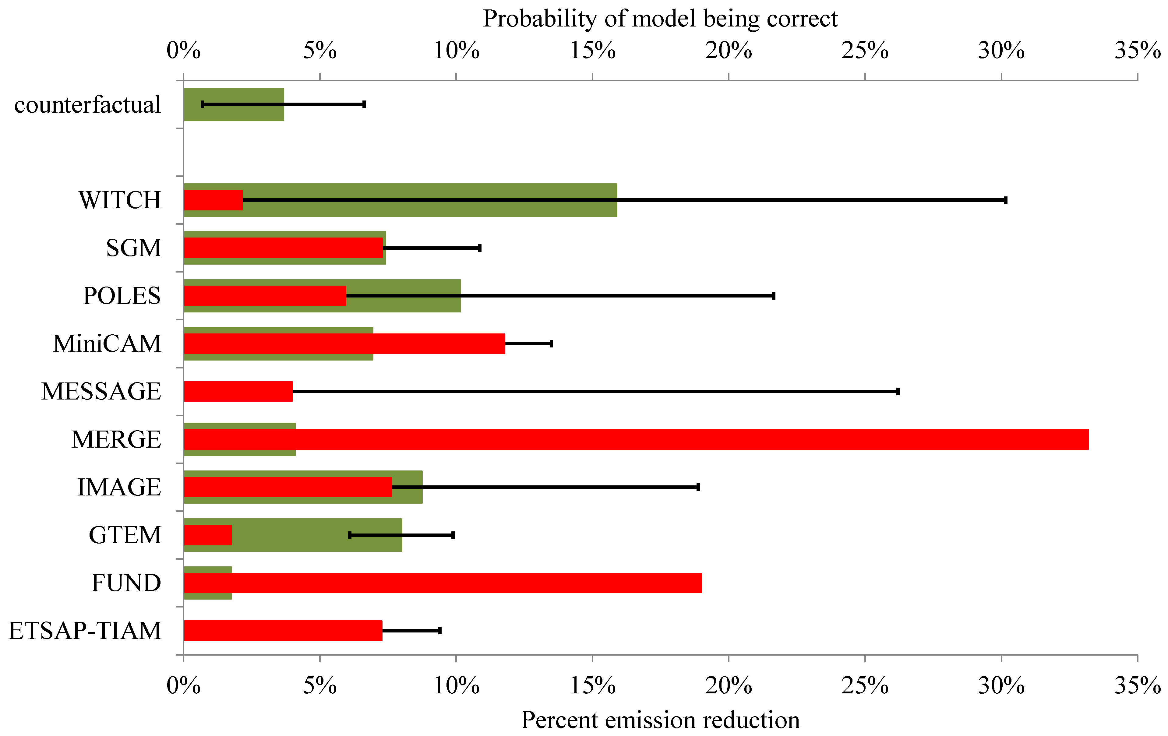
Figure 2 shows the estimated emission reduction; see also Table 1. It also shows the emission reduction from the baseline predicted by each model (or, rather, by the statistical emulator of each model). The two bottom-up models, ETSAP-TIAM and MESSAGE, find that the initial response to a carbon tax is an increase in emissions; note that this is not the case for their statistical emulators. The counterfactual one suggest that this is unlikely to have been the case: emissions fell because of the EU ETS. The remaining eight models predict an emission reduction, ranging from 1.7% for FUND to 16% for WITCH. The standard deviations vary widely, too, from 0.3% for FUND to 14% for MESSAGE.

Model performance as defined here follows from a combination of accuracy and precision, where accuracy is defined as “forecast” skill and precision as the standard deviation of the parameter estimate of the marginal cost function. A precisely accurate forecast is rewarded; a precisely inaccurate one punished. However, imprecise forecasts do well, too, as these are not wrong, just vague.

MERGE is the best performing model, with a 33% chance of being correct, followed by FUND (19%) and MiniCAM (12%). See Table 1. The models that do worst are WITCH (2.2%) and GTEM (1.8%). POLES, the model used by the European Commission, has a 6.0% chance of being correct.

Figure 2. The estimated emission reduction (due to the observed $13/tCO₂ carbon price; dark green bar at the top), the predicted emission reduction per model (or rather its statistical emulator; dark green bars), and the probability of the model being correct (light right inset); the lines indicate the 95% confidence interval.

Figure 2. The estimated emission reduction (due to the observed $13/tCO₂ carbon price; dark green bar at the top), the predicted emission reduction per model (or rather its statistical emulator; dark green bars), and the probability of the model being correct (light right inset); the lines indicate the 95% confidence interval.

3.4. The Carbon Price in 2030

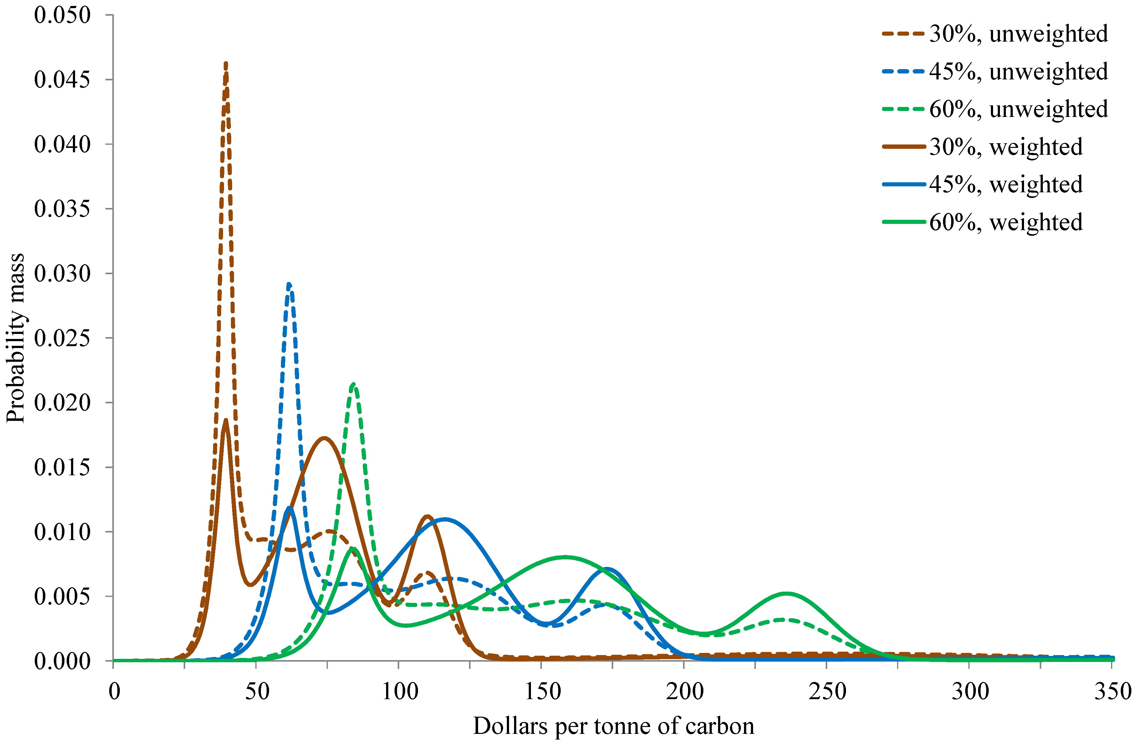
Figure 3 shows the joint probability density functions of the carbon price in 2030. The only uncertainty considered is the uncertainty about the costs of meeting any target. The pdfs in Figure 3 add up the pdfs of the ten individual models. In one case, the models are treated as equals; each has a weight of 1/10. In the other case, the models are weighted according to their ability to predict the impact of climate policy between 2005 and 2012. See Table 1. Separate pdfs are shown for each of the three emissions targets discussed above.

The unweighted pdfs show a sharp peak around low carbon prices and a long tail of higher prices. The weighted pdfs heavily discount the lower carbon prices and, instead, show a trimodal distribution around the best performing models.

Table 2 shows the mean and standard deviation of the carbon price in 2030. The carbon price rises steadily with the stringency of the target; for the weighted pdf, the carbon price is $87/tCO₂ for the 30% target, $137/tCO₂ for the 40% target and $187/tCO₂ for the 50% target. The total carbon tax revenue equals 1.2% of GDP in 2030 for the 40% target [20].

Figure 3. The probability density functions of the carbon prices, weighted and unweighted, needed for a 30%, 40% and 50% emission reduction (from base year 1990) in 2030.

Figure 3. The probability density functions of the carbon prices, weighted and unweighted, needed for a 30%, 40% and 50% emission reduction (from base year 1990) in 2030.

Table 2. The mean (and standard deviation) of the marginal and total costs of emission reduction in 2030 for three alternative targets and two alternative pdfs; also shown are the risk and ambiguity premiums on the total costs and the differences between results for the alternative pdfs.

pdf	Unweighted			Weighted
Target	−30%	−40%	−50%	−30%	−40%	−50%
Carbon price ($/tCO2)	82.9	130.4	178.0	86.9	136.7	186.6
	(65.5)	(103.2)	(140.8)	(55.6)	(87.6)	(119.5)
Total cost (%GDP)	0.11%	0.26%	0.48%	0.11%	0.27%	0.51%
	(0.08%)	(0.21%)	(0.38%)	(0.07%)	(0.17%)	(0.33%)
Risk premium (%GDP)	0.00003%	0.00021%	0.00074%	0.00002%	0.00015%	0.00054%
difference				28.0%	28.0%	28.0%
Ambiguity premium (%GDP)	0.00008%	0.00052%	0.00183%	0.00008%	0.00051%	0.00176%
difference				3.5%	3.6%	3.7%

Table 2. The mean (and standard deviation) of the marginal and total costs of emission reduction in 2030 for three alternative targets and two alternative pdfs; also shown are the risk and ambiguity premiums on the total costs and the differences between results for the alternative pdfs.

pdf	Unweighted			Weighted
Target	−30%	−40%	−50%	−30%	−40%	−50%
Carbon price ($/tCO2)	82.9	130.4	178.0	86.9	136.7	186.6
	(65.5)	(103.2)	(140.8)	(55.6)	(87.6)	(119.5)
Total cost (%GDP)	0.11%	0.26%	0.48%	0.11%	0.27%	0.51%
	(0.08%)	(0.21%)	(0.38%)	(0.07%)	(0.17%)	(0.33%)
Risk premium (%GDP)	0.00003%	0.00021%	0.00074%	0.00002%	0.00015%	0.00054%
difference				28.0%	28.0%	28.0%
Ambiguity premium (%GDP)	0.00008%	0.00052%	0.00183%	0.00008%	0.00051%	0.00176%
difference				3.5%	3.6%	3.7%

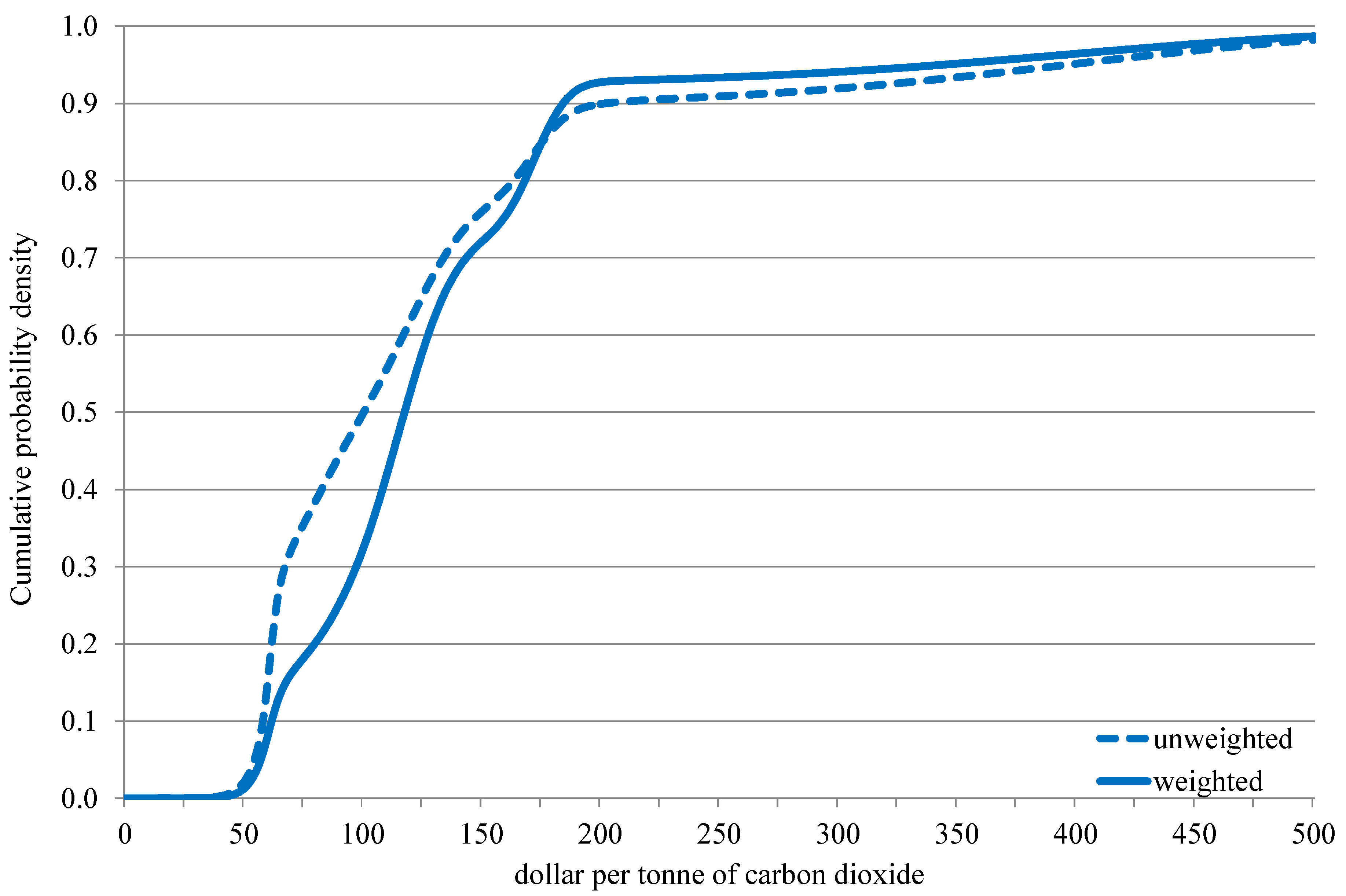
There is little difference between the weighted and unweighted pdf; for the 40% target, the unweighted mean is $130/tCO₂. Figure 3 shows that the mode is very different, but this does not carry over to the mean. Figure 4 shows why. The unweighted pdf lies generally to the left of the weighted pdf, but it has a much fatter right tail. The weighting with predictive power also discounts the very diffuse models (including their right tail).

Figure 4. The cumulative density functions, weighted and unweighted, for a 40% emission reduction (from base year) in 2030.

Figure 4. The cumulative density functions, weighted and unweighted, for a 40% emission reduction (from base year) in 2030.

3.5. The Costs of Meeting the 2030 Targets

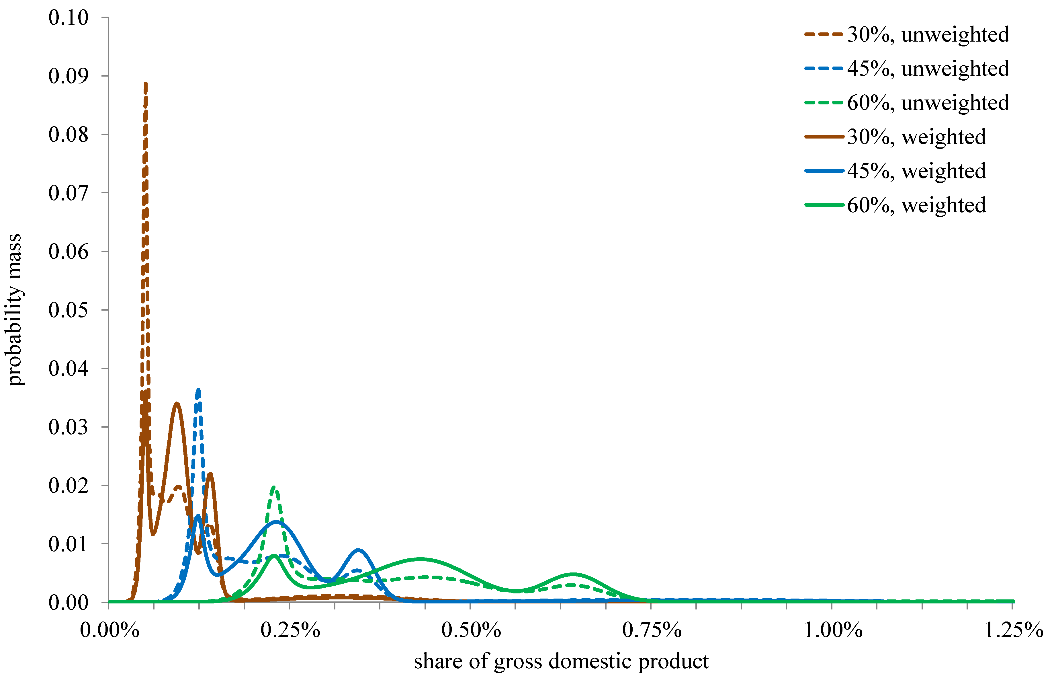
Figure 5 shows the pdfs of the total costs (in 2030) of meeting the emissions targets for 2030. The uncertainty about both the marginal and the total cost is driven by the uncertainty about the unit cost, so Figure 5 looks much like Figure 3, except that the distance between the different targets is larger, as total costs are assumed to be quadratic in emission reduction, whereas marginal costs are linear.

Table 2 shows the mean and standard deviation of the total cost. The costs rise rapidly with the stringency of the target; for the weighted pdf, the policy cost is 0.11% of income for the 30% target, 0.27% for the 40% target and 0.51% for the 50% target. The difference between the weighted and unweighted pdf is again small, for the same reason as above; for the 40% target, the mean of the unweighted pdf is 0.26%.

3.6. Risk and Ambiguity Premiums

Table 2 shows the risk and ambiguity premiums on the total cost of greenhouse gas emission reduction in 2030. The risk premium is the difference between the certainty equivalent impact and the expected impact. The certainty equivalent impact is the monetised welfare impact under certainty that equals the expected welfare impact (without ambiguity aversion). The ambiguity premium is the difference between the risk premiums with and without ambiguity. The clarity equivalent is the monetised welfare impact under certainty that equals the expected welfare impact under ambiguity. See [21].

Figure 5. The probability density functions of the total costs, weighted and unweighted, of a 30%, 40% and 50% emission reduction (from base year) in 2030.

Figure 5. The probability density functions of the total costs, weighted and unweighted, of a 30%, 40% and 50% emission reduction (from base year) in 2030.

The risk premiums are small, which is no surprise, as the impacts are small and per capita income is high. The risk premiums rise with the stringency of the emissions target and much faster so than the expected impacts. This is again as expected, since both the mean and the spread of the costs increase with the stringency of the target. The weighted risk premium is smaller than the unweighted risk premium; the certainty equivalents are thus closer together than the means. The principal reason is that the highest and most diffuse cost estimate is discounted by the data.

The weighted ambiguity premiums are smaller than the unweighted ones, for the same reason as above. The ambiguity premiums rise with the stringency of the emissions target and faster than the certainty equivalents. The reason is as above: the ambiguity premium puts further emphasis on improbable cost estimates. The ambiguity premiums are small, because the impacts are small and per capita income is high.

The mean total impact is 4.6% lower for the weighted pdf, and the certainty equivalent is 28% lower. These differences are independent of the stringency of the target. This is because the uncertainty is about the unit cost parameter, and without ambiguity aversion, the joint pdf is a linear combination of the individual pdfs that is independent of the point at which the expectation is taken.

This is not the case for the clarity equivalent: the weighted clarity equivalent is 3.5% below the unweighted one for the least stringent target and 3.7% for the most stringent target.

The reduction in certainty equivalent is larger than the reduction in the mean impact, because the disutility of improbably large costs is emphasized. The reduction in the clarity equivalent is smaller because it is, in essence, a certainty equivalent of the certainty equivalent. The first certainty equivalent absorbs the tails. The clarity equivalent absorbs the uncertainty acrossmodels, which, in this case, is much smaller than the uncertainty about each model.

4. Discussion and Conclusions

In this paper, I estimate the costs of meeting the EU 2030 targets for greenhouse gas emission reduction. Instead of using a single model, I use statistical emulators of ten different models. This allows for an analysis of both uncertainties and ambiguities. The estimated costs are relatively small, a tenth of the percent of GDP for the −40% target. Consequently, and because the inhabitants of the EU are rather rich on average, risk and ambiguity premiums are small, too. I test the models against the estimated impact of actual climate policy and find that some models, including the ones often used in official studies, perform much worse than others. Weighting the model results by their past performance does not lead to a substantial change in the estimated costs, but it does increase confidence.

There are a number of caveats. This paper is a proof of concept rather than a definitive estimate. The analysis should be done with the actual models, rather than with statistical emulators, realizing that a statistical interpretation of simulation models is not straightforward. Results could vary if important details of either baseline projections or policy implementation differ between the studies used for estimating the emulators and the cases considered here. The analysis is limited to one region and one period; models that perform badly in this paper may do well in other places or times. My estimate of the counterfactual emissions in the EU is rough and ready and could be improved by decomposition analysis. Sectoral detail is lacking, and the econometrics are simple, not controlling for energy prices, business cycle, renewable mandates and other climate and energy policies.

The ideas offered here are worth considering nonetheless. Models of the costs of climate policy can be tested against actual climate policy. This guides modellers towards assumptions and specifications that require revision. It informs policy makers about which models are the more reliable ones.