1. Introduction
Post-industrialized economies rely on energy for almost all fundamental needs including food production, heat, transportation, manufacturing, and communication. Since the Industrial Revolution, fossil energy resources such as coal, petroleum, and natural gas have become the dominant sources of energy because they are readily accessible and inexpensive. The use of fossil fuels have enabled large-scale industrial development, but growing concerns regarding energy security and the environment, particularly climate change, have inspired the development of mandates for renewable energy from wind, biomass, and solar energy sources. In the United States for example, by 2022, the Energy Independence and Security Act (EISA) of 2007 requires that 61 billion L/year cellulosic ethanol replace petroleum-based transportation fuels. To meet this demand, an estimated 242 million Mg/year of biomass will need to be supplied to biorefineries that can process lignocellulose [
1]. Sufficient biomass supply has been identified to meet these requirements through large-scale national assessments [
2], and research is on-going concerning the logistics required to cultivate, harvest, transport, and process such large quantities of biomass into fuel. Our study focuses on the supply and logistics chain of the lignocellulosic ethanol produced from corn stover, an agricultural residue.
Biomass supply chains currently use equipment and infrastructure designed for existing agriculture and forest industries. These supply chains are designed to move biomass short distances, store it for limited periods of time, and are constrained in their ability to address biomass quality issues like moisture and ash content. Most widely cited lignocellulosic biorefinery designs [
3,
4,
5,
6] that utilize agricultural residues (e.g., corn stover) or dedicated energy crops (e.g., switchgrass) for biochemical conversion to alcohol have been designed and priced to take in baled biomass feedstocks, assuming the existing (conventional) infrastructure. Although these conventional systems are cost-effective in high biomass-yielding areas, such as supplying corn stover in Iowa or forest resources in the Alabama, they are limited in their ability to support and meet long term national biofuels production goals [
7]. For example, there are ample biomass resources that would be considered stranded under this model due to having a high transport distance that would result in prohibitive costs. A strong driver for the conventional system is to minimize transportation costs as biomass characteristics make them expensive to handle and transport. Examples of these characteristics include high moisture content, low bulk density, low energy density, high variability, and multiple formats. Richard [
8] reviewed the challenges of establishing bioenergy systems from low energy-density biomass resources and discusses different technologies for increasing the energy density of agricultural feedstocks through different preprocessing steps, including pelleting, pyrolysis, and torrefaction. Such densification systems may be more appropriate for thermochemical (e.g., torrefaction and pyrolysis) as opposed to biochemical (pelleting) conversion. One approach to addressing these challenges for biochemical conversion platforms, while also bringing in stranded resources and reducing risk to the biorefinery, is to transition to a commodity-based feedstock supply system, such as that proposed by Idaho National Laboratory (INL) [
7]. The commodity system incorporates distributed biomass preprocessing depots located near the point of production. The depots can provide the biorefineries with a quality-controlled biomass supply, which is sourced from a variety of biomass types [
9]. Based on the availability of sufficient corn stover in Kansas to meet the biorefinery’s capacity (2000 dry metric tons/day based on the work of [
6]), the biorefinery could take in corn stover feedstock to meet annual supply. In the commodity system, the variability in feedstock characteristics such as moisture and ash content can be addressed by the local preprocessing depot to therefore supply the biorefinery with a dense, stable, quality controlled feedstock [
8].
Most life cycle assessment (LCA) studies of biochemically-derived ethanol from lignocellulose have assumed the conventional model of delivering baled biomass (for agricultural residues or dedicated energy crops/purpose-grown grasses) directly to the lignocellulosic biorefinery [
10,
11,
12,
13,
14]; however, recent LCA literature has compared conventional and commodity systems. Eranki
et al. [
15] compared the energy inputs and greenhouse gas (GHG) emissions of commodity and conventional systems delivered to a 5000 ton/day centralized biorefinery. The commodity system consists of nine preprocessing depots with a fixed capacity (500 tons/day). The mass fraction of biomass feedstock (corn stover, switchgrass and miscanthus) was varied in order to account for the uncertainty in energy requirements for feedstock production. The study concluded that the commodity system’s GHG emissions are about 4% lower, while consuming approximately the same total energy as the conventional system. The study also emphasized that the processing technology was critical to cost-reduction for the commodity system, a point also addressed by Shastri
et al. [
16] and Uria-Martinez
et al. [
17]. Recently, Argo
et al. [
18] evaluated several environmental sustainability impacts (100-year global warming potential (GWP), rainfall (green water) and groundwater through irrigation (blue water) footprints), and costs for advanced logistics designs that employ densification steps for preprocessing agricultural residues and grasses in depots for long-haul transport to centralized biorefineries designed on the biochemical platform. Their results showed that the commodity system reduced both spatial and temporal variability and thus stabilized the cost of the feedstock logistics and supply chain. Egbendewe-Mondzozo
et al. [
19] analyzed the cost and GHG emissions of conventional and commodity systems practiced in Southwest Michigan. The supply and logistics chain of the commodity system included seven preprocessing depots located in nine counties, and a centralized biorefinery. The authors examined different processing technology in order to evaluate their effects on biofuel production cost and energy inputs. The study concluded that the commodity system reduced the net life cycle GHG emissions; however, the profitability varied with the type of biomass feedstock and processing technology. Ray
et al. [
20] and Hess
et al. [
21] tested the effects of corn stover pellet densification on low- and high-solids pretreatment performance within biochemical conversion systems. The study concluded that pelletizing corn stover did not have a negative impact on pretreatment efficacy. Limited investigation from literature on the effects of densified feedstock on downstream processes suggests there is no adverse impact or possible improvement on pretreatment efficacy [
22,
23,
24].
Select literature has examined spatial contributions to life cycle environmental impacts of ethanol from different feedstocks, mainly pertaining to the infrastructure and logistics of moving the product (ethanol fuel) to demand centers. For example, Wakeley
et al. [
25] concluded that at higher production scales, ethanol long-haul transport costs and environmental emissions would decline through use of rail infrastructure to transport due to the majority of supply (in the Midwest) needing to access demand centers (on east and west coasts of the U.S.). Strogen and colleagues evaluated the costs and emissions of bio-ethanol distribution on a larger scale than previously studied, and concluded that annual ethanol production scale critically impacts the average transport distance to end use markets [
26]. The authors found that more than 300,000 tons of CO
2e could be avoided if all unnecessary transportation were eliminated. Moreover, Argo
et al. [
18] found that the logistics of the commodity system results in lower production costs than the conventional one when the biorefinery capacities are above 5000 Mg/day. A study by INL acknowledged that the transportation cost savings in the commodity system does not completely offset the costs associated with the pelleting and regrinding at all transport distances. If the benefits of handling and storing pellets are quantified, the transportation cost savings can be increased and thus can balance or exceed the cost of densification. However, the total cost of the commodity supply chain system could be higher than the conventional system due to the addition of preprocessing operations and equipment [
16,
27]. Our objective is to evaluate the spatial variability of life cycle environmental impacts owing to characteristics along the biomass feedstock supply chain (
i.e., from field to depot to biorefinery with intermediate transportation and preprocessing steps) that incur variability as a result of the quantity of biomass harvested, collected, stored, moved, and preprocessed prior to long-distance transport to a centralized biorefinery. Thus, our focus is on identifying processes within the feedstock logistics sequence that introduce the most significant uncertainty in life cycle impact assessment (LCIA). We focus on one LCIA metric, the 100-year GWP applied to a case study of a commodity system design in the state of Kansas (United States) through several configurations for depot location siting, and discuss the relevance to other important environmental impacts within agricultural bioenergy supply systems. Kansas was chosen in INL’s 2017 [
28] design report as an area that could support a uniform format “depot” supply system design mainly because of resource density (
i.e., the presence of sufficient biomass supply) and mix of different feedstocks in different supply regions of the U.S. Our study focuses on Kansas in order to leverage assumptions from INL’s 2017 report for the Midwest region, whose supply of corn stover could support depots supplying biomass commodities to a centralized biorefinery; and to demonstrate the depot design where it may likely take place, given resource availability
. Our specific objective in this paper is to evaluate the uncertainty in life cycle GWP of the harvest, collection, storage, preprocessing, and transportation stages with two different configurations of depot size and location, whereby the location, size, and number of depots for a particular feedstock supply system design may incur significant dominance and/or variability to the life cycle GWP.
2. Methods
LCA, following the International Organization for Standardization (ISO) 14040 methods [
29], was applied to evaluate environmental aspects of the bio-ethanol logistics and supply chain. Data for the life cycle inventory (LCI) model, which include the energy resources consumed to process corn stover at different scales, were derived using simulations from the Biomass Logistics Model (BLM) developed using Powersim™ at INL (Idaho Falls, ID, USA) [
27]. The BLM incorporates information from a number of databases which include all the data related to: (1) the engineering performance data of biomass pre-processing equipment; (2) labor costs; and (3) local tax and regulation data [
27]. ArcGIS was employed in this study in order to site the biorefinery and preprocessing depots and define all transportation distances [
30]. The spatial data are publicly available on the website of the Aerial Photography & GIS Data for the Professional & Novice (for counties) [
31], and the Kansas Data Access & Support Center (DASC) (for railroads and highways) (Lawrence, KS, USA) [
32,
33]. We use an attributional LCA (aLCA) approach in this study to investigate the spatial variability in LCIA metrics; however, we note the limitations of this approach raised by Andersen [
34], who discussed potentially negative environmental impacts resulting from agricultural residue diversion, in that case, bagasse, for biofuel production.
Through a focused analysis of agricultural residue harvest, collection, storage, transport, and preprocessing, this study builds on prior work aimed at understanding and characterizing uncertainties within the life cycle supply chain of lignocellulosic ethanol (bio-ethanol) [
13,
35,
36]. With the exception of a recent study [
18], most prior LCA studies of bio-ethanol [
10,
11,
13,
14,
37] have assumed a conventional harvest and biomass delivery in bale format, resulting in relatively low (approximately 10%) net life cycle GHG emissions [
11]. Here, we focus on identifying and characterizing uncertainties in advanced agricultural residue harvest, collection, storage, transport, pre-processing, and delivery operations to bio-ethanol facilities in the U.S. Midwest that arise due to variability in: (1) the sustainable harvest yield, defined as the quantity of corn stover removal set to maintain erosion and soil carbon within tolerable levels [
2]; (2) transportation of the agricultural residue to depots that process and densify the biomass; (3) depot facility size, which influences equipment and energy throughput per unit of biomass; and (4) long-distance transport of the densified biomass delivered to the bio-ethanol facility. While we note the significant variability in GHG emissions from feedstock production noted in literature, and in particular the possible risks to loss of soil organic carbon (SOC) with corn stover removal [
38,
39], here we focus exclusively on uncertainties that could arise due to the spatial variability of corn stover feedstocks available at different spatial densities in the U.S. Midwest.
The commodity system allows lignocellulosic biomass to be traded and supplied to biorefineries in a commodity-format market. A number of preprocessing depots can be located within or around the vicinity of biomass and are deployed to convert a diverse, low-density, perishable feedstock resource into an aerobically stable, dense, uniform-format [
9,
21]. The preprocessing steps and equipment include: loaders, horizontal grinders, grinder in-feed systems, and dust collection and conveyor systems [
7,
9]. The energy sources for depot equipment are described in
Table S1. A commodity system and depots would likely first appear in areas without enough resources to supply a single biorefinery, requiring resources to be brought in beyond the local area. The incorporation of depots would allow stranded resources to enter the system which would otherwise be economically inaccessible. For this reason, corn stover located in the state of Kansas outside of high yielding areas within the U.S. corn-belt was chosen for analysis.
2.1. Life Cycle Assessment of the Corn Stover to Lignocellulosic Ethanol Logistics and Supply Chain
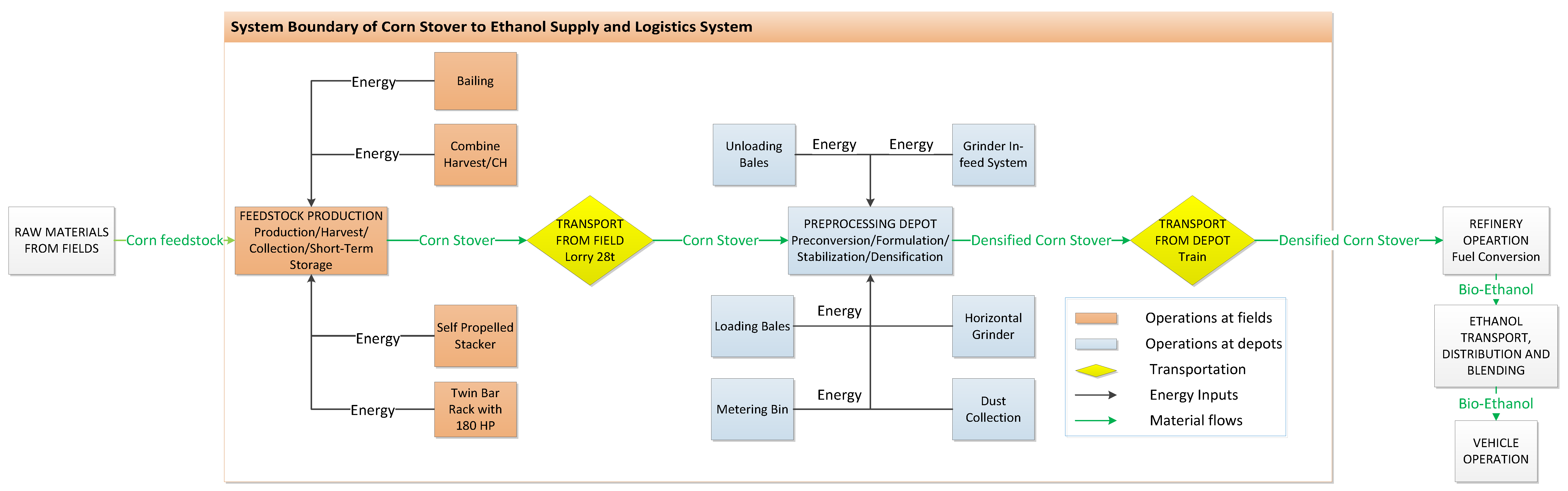
A LCA model was developed to evaluate uncertainties in GHG emissions for a corn stover-to-ethanol commodity system. A gate-to-gate LCI model was developed followed by LCIA evaluation of the 100-year GWP metric for corn stover feedstock logistics. The feedstock logistics we model in this work fits into a gate-to-gate segment of the full lignocellulosic ethanol life cycle (
Figure 1), which refers to the sequence of processes within the life cycle of biomass production, conversion, and in-use consumption. The system boundary for the full life cycle of corn stover-to-ethanol (
Figure 1) consists of: (1) feedstock production (
i.e., crop production including nutrient replacement and soil GHG emissions); (2) feedstock harvest, collection, and storage; (3) feedstock transport from field to biomass preprocessing depot; (4) preprocessing depot operations; (5) commodity transport from biomass preprocessing depot to biorefinery; (6) biofuel conversion at the biorefinery; (7) ethanol transport, distribution, and blending; and (8) vehicle operation. The functional unit of the analysis is 1 MJ of ethanol. We rely on literatures’ estimates for Segments 1, 6, 7, and 8 (see [
36,
40] for development of the biorefinery model and for discussion of biorefinery inputs, respectively). The assumptions from literature [
37] correspond to conventional biomass sourcing with on-site power production and an electricity credit from the Midwest electricity grid mix.
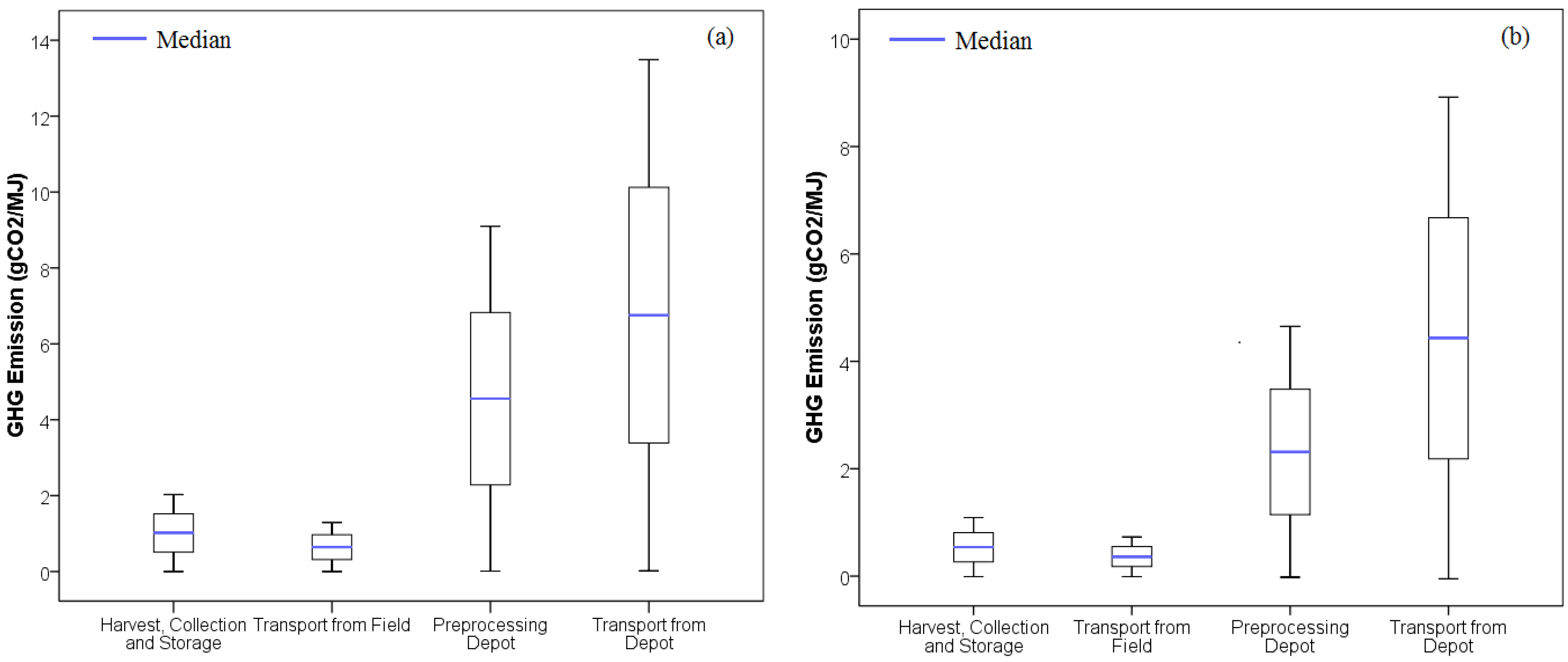
This paper focuses on identifying significant uncertainties in environmental metrics within an advanced logistics configuration of the corn stover-to-ethanol supply chain, which was designed to reduce transportation distance and costs. A single-variable sensitivity analysis was conducted to examine the significance of LCI model parameters for harvesting, transporting from field, preprocessing at the depot and transporting from the depot in the advanced commodity system. Commodity transportation (as baled corn stover or densified biomass) is a function of both transport distance and feedstock density.
Figure 1.
Gate-to-gate system boundary for the corn stover commodity feedstock supply and logistics system within the life cycle of bio-ethanol production.
Figure 1.
Gate-to-gate system boundary for the corn stover commodity feedstock supply and logistics system within the life cycle of bio-ethanol production.
2.2. Data Management and Analysis
ArcGIS tools were used to identify depot and biorefinery locations and to measure the transport distances within the commodity supply chain. The criteria for location selection consisted of the presence of transportation infrastructure (railroads and road systems) and annual biomass availability (
i.e., sustainable harvest yield) in the state of Kansas [
2]. Significant factors such as access to water, and availability of utilities and labor were assumed sufficient for the model scenarios constructed. For this study, factors affecting policy such as political districts, voting locations and school systems were not considered. Transportation data, including road and rail networks, and freight and truck stations, were obtained from the Aerial Photography & GIS Data for the Professional & Novice [
31] and the DASC [
32,
33]. Biomass supply data were assumed to correspond to the marginal access (farm-to-gate) cost, which is proportionally related to biomass demand. The US Department of Energy’s U.S. Billion-Ton Update Report (BT2) [
2] estimates biomass marginal access costs in $5/ton increments. For the counties we consider in Kansas, biomass marginal access costs begin at $40/ton and can be as high as $80/ton depending upon the available supply within each county. Wakeley
et al. [
25] and Argo
et al. [
18] varied biorefinery capacity in their studies in order to examine the range of transportation cost and GHG emissions. In this study, the biorefinery capacity was fixed at 800,000 dry matter tons (DMT)/year. The supply chain was designed to provide 900,000 DMT to account for possible losses due to the converting, handling and transporting processes. We assumed that multiple depots would feed one centralized biorefinery. Given these boundary conditions, a master map was developed joining all transportation and biomass availability data (
Figure S1). A radius of 80-km (50-miles) radius is assumed for feedstock transportation from the corn farms to the preprocessing depots. Several tools within ArcGIS were used to identify the geographic boundary of the LCI model. The centroid of each county was identified by using the Spatial Analysis (Feature to Point) tool. The ArcGIS Find Route tool was used to measure the rail distances between two locations based on the available railroad networks. The biomass supply data for each Kansas County were imported to ArcGIS and converted to raster format. The biomass supply data were presented in the master map in order to demonstrate the biomass density and distribution across Kansas. Two depot configurations were considered: (1) equal spatial distance between depots and infrastructure (rail network) availability; and (2) high biomass density and infrastructure (rail network) availability. The rationale for selecting the two configurations was to test the impact that the number of depots and their relative location within a biorefinery supply radius have on life cycle GHG emissions.
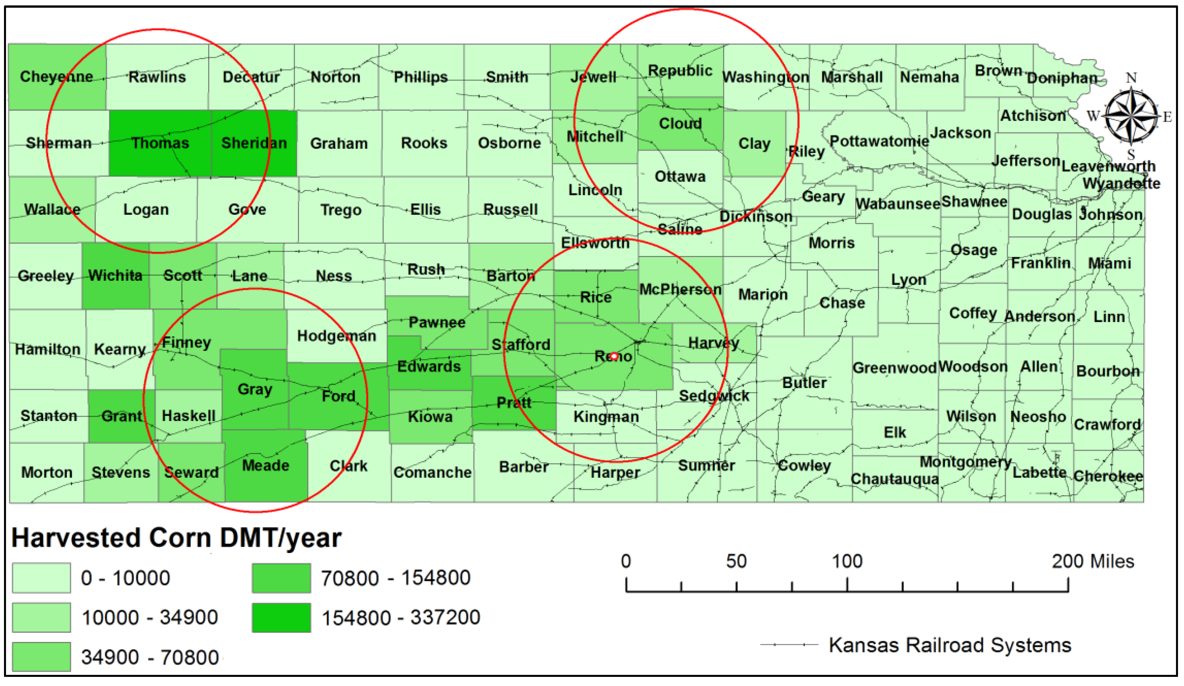
2.2.1. Configuration 1: Equal Spatial Distance between Depots and Infrastructure Availability
The first configuration divides the state of Kansas into six equally spaced primary regions: (1) Northwest; (2) North; (3) Northeast; (4) Southeast; (5) South; and (6) Southwest. However, according to resource assessment data from Oak Ridge National Laboratory (ORNL) [
2], the counties in Regions 3 and 4 would not supply biomass for ethanol production (
Figure S1). Therefore, counties in these regions were eliminated from the scope of analysis. Four depots are located in Regions 1, 2, 5, and 6 within the vicinity of biomass supply of each region. They are also cited close to road and rail transportation infrastructure to take in baled feedstock and export (via long distance) densified biomass (
Figure 2, spatial boundary). Note that the sizing criteria for depots used in this study are different than those used by INL.
Figure 2.
Scenario 1 depot configuration based on equal spatial siting between depots and infrastructure availability. The red circle shows the biomass supply radius. The depots are located at the center of the circle and receive feedstock from counties within an 80-km (50-miles) radius. The red point at the centroid of Reno County corresponds to the location of the biorefinery.
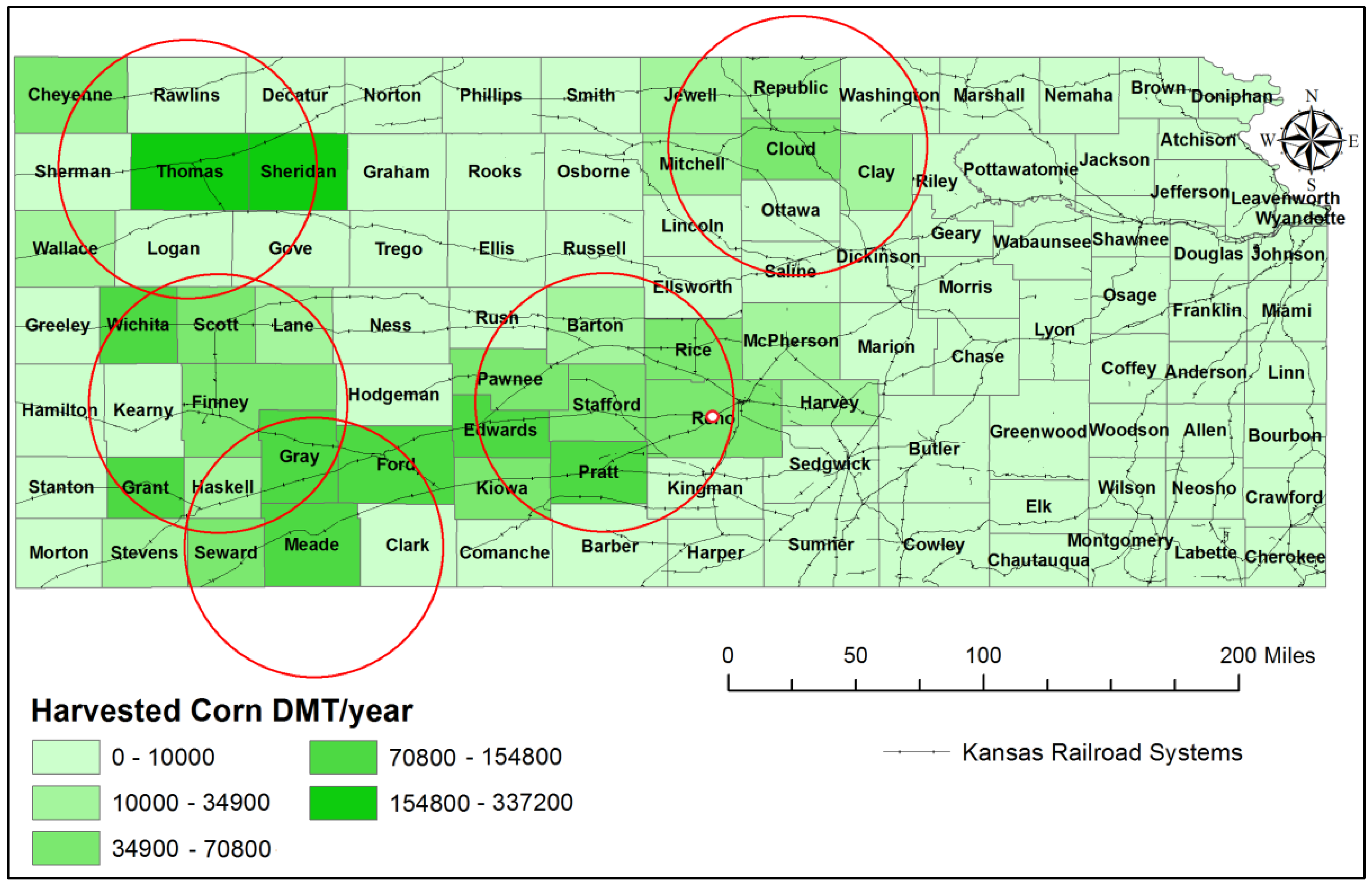
2.2.2. Configuration 2: High Biomass Density and Infrastructure Availability
The second depot configuration places depots according to biomass availability and the shortest railroad distance from the depot to the biorefinery, and is derived from the existing Kansas rail systems (
Figure 3) in the central-to-west range of the state. Argo
et al. [
18] assumed in their model that the feedstock was transported from field to depot by semi-truck and from depot to biorefinery by rail given that railcars are capable of carrying a greater volume of goods with the minimal variable cost per mile. Thus, we assumed that distribution by truck is preferred for transport from field to depot, and rail is preferred for long distance transportation from depot to biorefinery. Based on the distribution of biomass and feedstock transport distance from field to depot, five biomass preprocessing depots were located in the state in counties surrounded by dense feedstock supply.
Figure 3.
Scenario 2 depot configuration based on biomass density and infrastructure availability. The red circle shows the biomass supply radius. The depots are located at the center of the circle and receive the feedstock from counties within an 80-km (50-miles) radius. The red point at the centroid of Reno County corresponds to the location of the biorefinery.
2.2.3. Life Cycle Assessment Modeling Approach
The BLM inventories all equipment and transport modes used to process and move biomass from the field to the biorefinery reactor infeed [
29]. The transport distance, specified using ArcGIS software, and the depot capacity were varied and analyzed by the BLM model in order to generate the relative energy consumption from each field supplying feedstock to depot and densified biomass to biorefinery. The cumulative energy consumption in advanced logistics is the product of the normalized energy consumption from the BLM (in gallons of diesel per DMT), which includes a semi-truck (2.88 L) to transport one DMT of biomass and a baler (1.36 L) to compress one DMT of biomass, and the biomass input, which was scaled according to the depot capacity. Energy consumption data were input into the SimaPro V.7.3.3 LCI [
41] model in order to compute the life cycle GHG emission. The SimaPro model accounts for all upstream cradle-to-gate inputs of process energy (diesel and electricity). In order to expedite the gate-to-gate LCIA computation for the two scenarios, a Matlab script [
42] was written to batch-process the BLM energy and resource data outputs into SimaPro to generate the GHG emissions for the 46 supply counties (See
Section S4 for more detail).
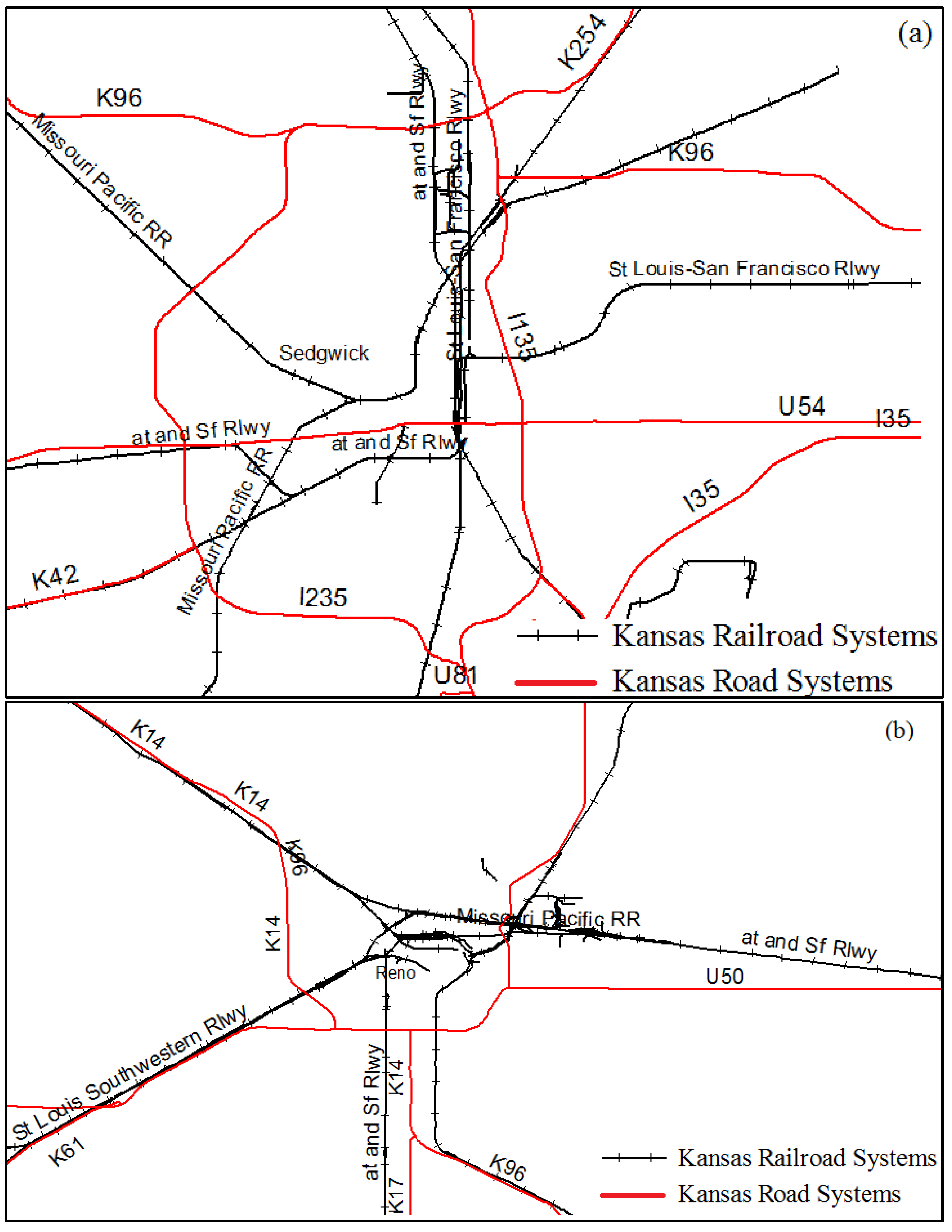
2.3. Biorefinery Location
The biorefinery was located in Reno County based on its proximity to road and railway infrastructure. Two counties were identified originally, Sedgewick (
Figure 4a) and Reno (
Figure 4b), given their location within the state being in areas with high highway and railway access. Reno County was selected based on it having five highways (K14, K17, U50, K61, K96) and four railroads (St. Louis Southwestern, Missouri Pacific and Atchison, Topeka & Santa Fe Railway and Chicago, Rock Island and Pacific Railroad), whereas Sedgewick has nine highways (I235, K96, I135, I35, K15, U54, U81, K42, K254) but a less extensive railway network of three railroads (Missouri Pacific, Chicago Rock Island, Pacific and St. Louis-San Francisco Railway). Thus, the biorefinery was sited in Reno County because of its proximity to the biomass supplying counties and because of its better access to four railroad networks that could facilitate access on energy efficient rail between depots and the biorefinery, thus giving access to all depot locations selected in Scenarios 1 and 2 (
Figure S1).
Figure 4.
Highway (red) and rail systems (black) of (a) Sedgewick County and (b) Reno County.
Figure 4.
Highway (red) and rail systems (black) of (a) Sedgewick County and (b) Reno County.
2.4. The Capacity of the Biomass Preprocessing Depots
The available biomass supply in Kansas exceeds the biorefinery feedstock demand of 900,000 DMT/year. The maximum capacity of each preprocessing depot is assumed to be less than 400,000 DMT/year in order to increase the network of the distribution systems. The depot size limitation allows for more depots to be distributed across the state to supply the annual constant corn stover needed for the centralized biorefinery. To be conservative, we set the size of the pre-processing depots based on the local feedstock density within an 80-km (50-miles) radius. A simple mathematical rule was applied to estimate the depot capacity (
Table S2 and
Table S3, and Equation (S1)) and farm supply (
Table S4 and
Table S5, and Equation (S2)) based on the availability of biomass supply. We assumed that neighboring counties would transport biomass to the nearest depot within an 80-km (50-miles) radius. The distance from the depot to the biorefinery is the distance from the centroid of the county with the depot to the centroid of the county with the biorefinery for Scenario 1 (
Table 1) and Scenario 2 (
Table 2). The sizing criteria for depots used in this study are different than that used by INL.
Table 1.
Preprocessing depot capacities and true rail distance from depots to the single biorefinery in Scenario 1. DMT: dry matter ton.
Table 1.
Preprocessing depot capacities and true rail distance from depots to the single biorefinery in Scenario 1. DMT: dry matter ton.
| Depot locations | Depot capacity (DMT/year) | Transport rail distance |
|---|
| Thomas | 390,000 | 349 |
| Cloud | 50,000 | 160 |
| Gray | 275,000 | 142 |
| Reno | 185,000 | 14 |
| Total | 900,000 | 665 |
Table 2.
Preprocessing depot capacities and true rail distance from depots to the single biorefinery in Scenario 2.
Table 2.
Preprocessing depot capacities and true rail distance from depots to the single biorefinery in Scenario 2.
| Depot locations | Depot capacity (DMT/year) | Transport rail distance |
|---|
| Thomas | 295,000 | 349 |
| Finney | 190,000 | 176 |
| Meade | 150,000 | 136 |
| Stafford | 220,000 | 47 |
| Cloud | 45,000 | 160 |
| Total | 900,000 | 868 |
2.5. Uncertainty Analysis
We use Monte Carlo methods [
43,
44] to project the range of probable life cycle GWPs for the two scenarios. The gate-to-gate LCIA model developed in SimaPro V.7.3.3 estimates the GHG emissions (GWP) based on the energy resource inputs derived from the BLM. SimaPro GWP output data for each process in the supply chain were best fit to probability distributions using Oracle Crystal Ball Statistical Software (Oracle Corporation, Redwood City, CA, USA) [
45] and two distributions for Scenarios 1 and 2, respectively, were aggregated (
Figure S2 and
Figure S3). With the scenario probability distributions, a Monte Carlo Simulation (1000 iterations) was run to generate stochastic GWP estimates (
Table S6, and
Figure S2 and
Figure S3). The statistical mean, range, and probability distributions for the stochastic input processes (feedstock harvest, collection and storage, feedstock transport, preprocessing, and commodity transport) are noted in
Table S7. This uncertainty analysis procedure was adopted from Venkatesh
et al. [
46], who investigated uncertainties in life cycle GWP of U.S. coal; the authors fit probability distributions to coal model parameter inputs and used Monte Carlo simulation to examine the effect of spatial and temporal variability on life cycle GWP. Finally, we used single-variable sensitivity analysis to determine the relative significance of the four logistics gate-to-gate processes with respect to the final GHG emission given the expected low and high ranges in order to understand the variability within the system boundary and thus evaluate and mitigate potential environmental risks as noted by Venkatesh
et al. [
46].
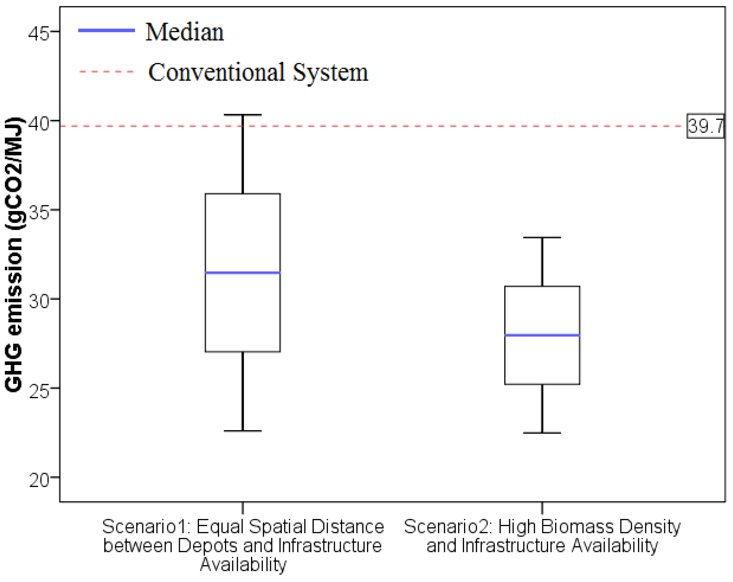
4. Conclusions
This study examines the variability in life cycle GHG emissions of a bio-ethanol feedstock logistics supply chain in Kansas, specifically examining uncertainties in advanced commodity systems that are found to mitigate risks associated with weather, pests, and disease [
18,
27]. In this study, the uncertainty in agricultural residue (corn stover) logistics was examined by testing the location siting and sizing of pre-processing depots in two different but plausible supply chain configurations in the state of Kansas. In Scenario 1, the depots were equally spaced and sited within the vicinity of counties that have high biomass supply density. In Scenario 2, the depot siting was leveraged to consider the shortest rail transport distance to a centralized biorefinery while considering the vicinity of high biomass supply counties. The stochastic results show that the GHG emissions for Scenario 1 have a wider variability and higher mean emissions (See
Table S9) than those of Scenario 2. This result illustrates the benefit of locating preprocessing depots in the vicinity of direct railroad lines to the biorefinery since rail transportation has the least environmental impacts and lowest costs [
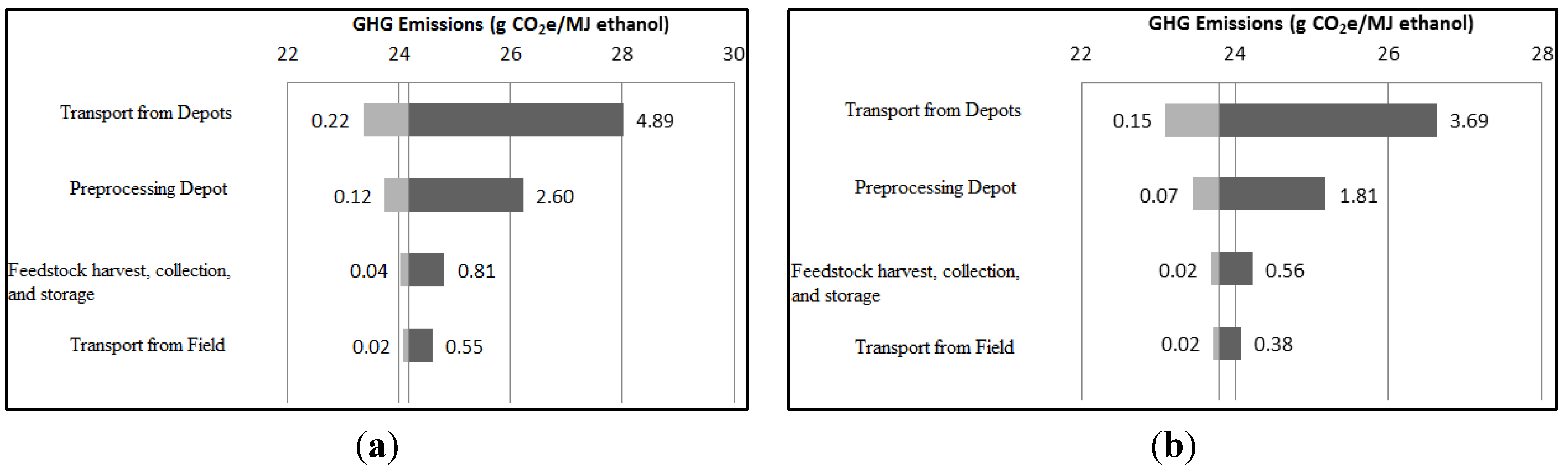
27]. It demonstrates that we expect to find a range of environmental impacts (in this case, GHG emissions) depending upon the quantity of biomass moved and upon the distance from biomass-supplying farms to preprocessing depots and from depots to biorefinery central facilities. Other environmental LCIA metrics that depend on energy consumption are expected to follow the variability trend exhibited by GHG emissions.
The depot-to-biorefinery transportation segment makes the largest contribution to life cycle GHG emissions from logistics and to life cycle GHG uncertainty for both scenarios. This suggests that the transport distance and the volume of transported commodity from depots are the significant parameters for supply regions like Kansas that have sufficient biomass supply in a feedstock commodity supply chain. Results may be quite different in regions that have many stranded biomass resources that need to be transported a long distance and collected at smaller centralized depots, the siting of which could depend on the presence of both road and rail infrastructure. Results also suggest that the uncertainty in GHG emissions of the depot-to-biorefinery and the pre-processing depot processes declines with increasing number of depots in a region. Future uncertainty analysis for feedstock logistics should focus on improving some of the model boundary settings, particularly the feedstock supply radius and the depot sizing method. The variability in the field-to-depot stage is minimized because the feedstock supply is limited to the region within an 80-km (50-miles) radius and thus the transport distance is assumed to be uniform. However, restricting the feedstock collection radius may impose a limitation in meeting biofuels production as noted by Argo
et al. [
18]. Therefore, future work should consider a larger biomass supply radius. In our study, the depot capacity was simply determined based on the feedstock supply ratio; however, a more precise optimizing of depot capacity could be used to test its significance on uncertainty in logistics chains that may require multiple stranded supply locations using a variety of lignocellulosic sources needed to fit a biorefinery’s annual supply wheel.


