Lorenz Wind Disturbance Model Based on Grey Generated Components

Abstract
:
1. Introduction
2. Nonlinear Lorenz Disturbance and Data Preprocessing Forms
2.1. Different Types of Lorenz Disturbance and Normalization Constants
2.1.1. Different Types of Disturbance in a Lorenz System

| Items to be Compared | The Values of r and its Corresponding Fluid Motions | |||
|---|---|---|---|---|
| Rayleigh Number (r) | 0 < r < 1 | 1 < r < 13.97 | 13.97 < r < 24.74 | r > 24.74 |
| Actual fluid motion | Heat conduction | Regular convection | Transient chaos | Chaos |
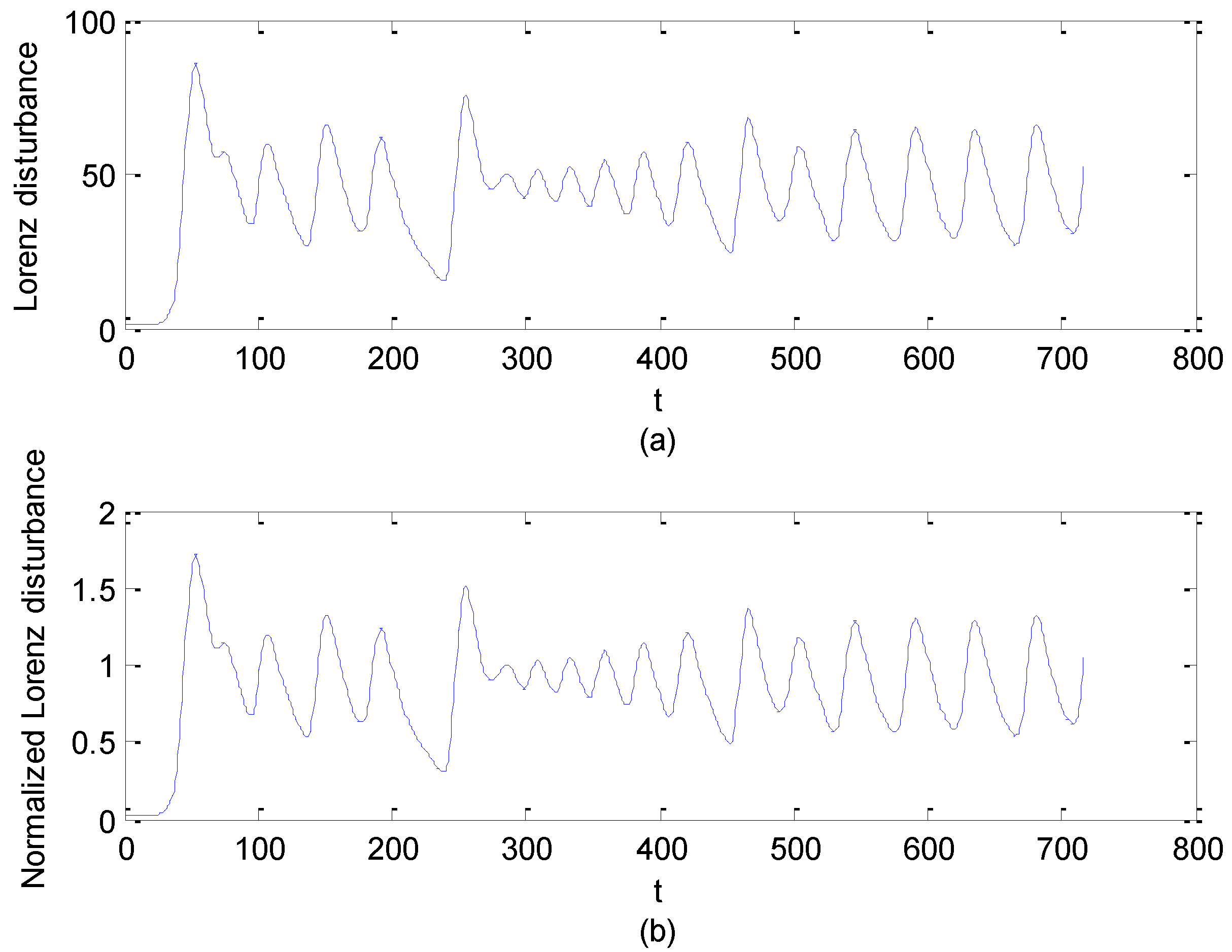
2.1.2. Normalization Constant of Lorenz Disturbance

2.2. Data Preprocessing


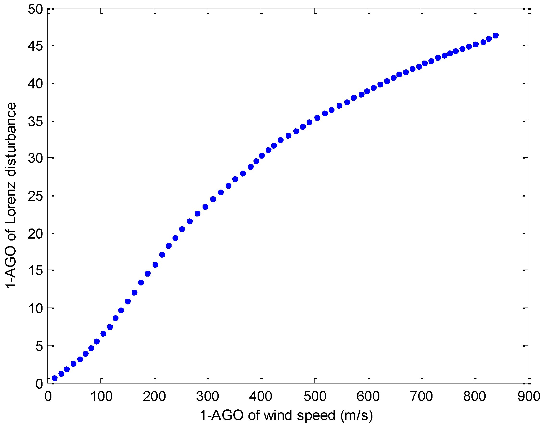
3. Wind Disturbance Model Based on Grey Generation
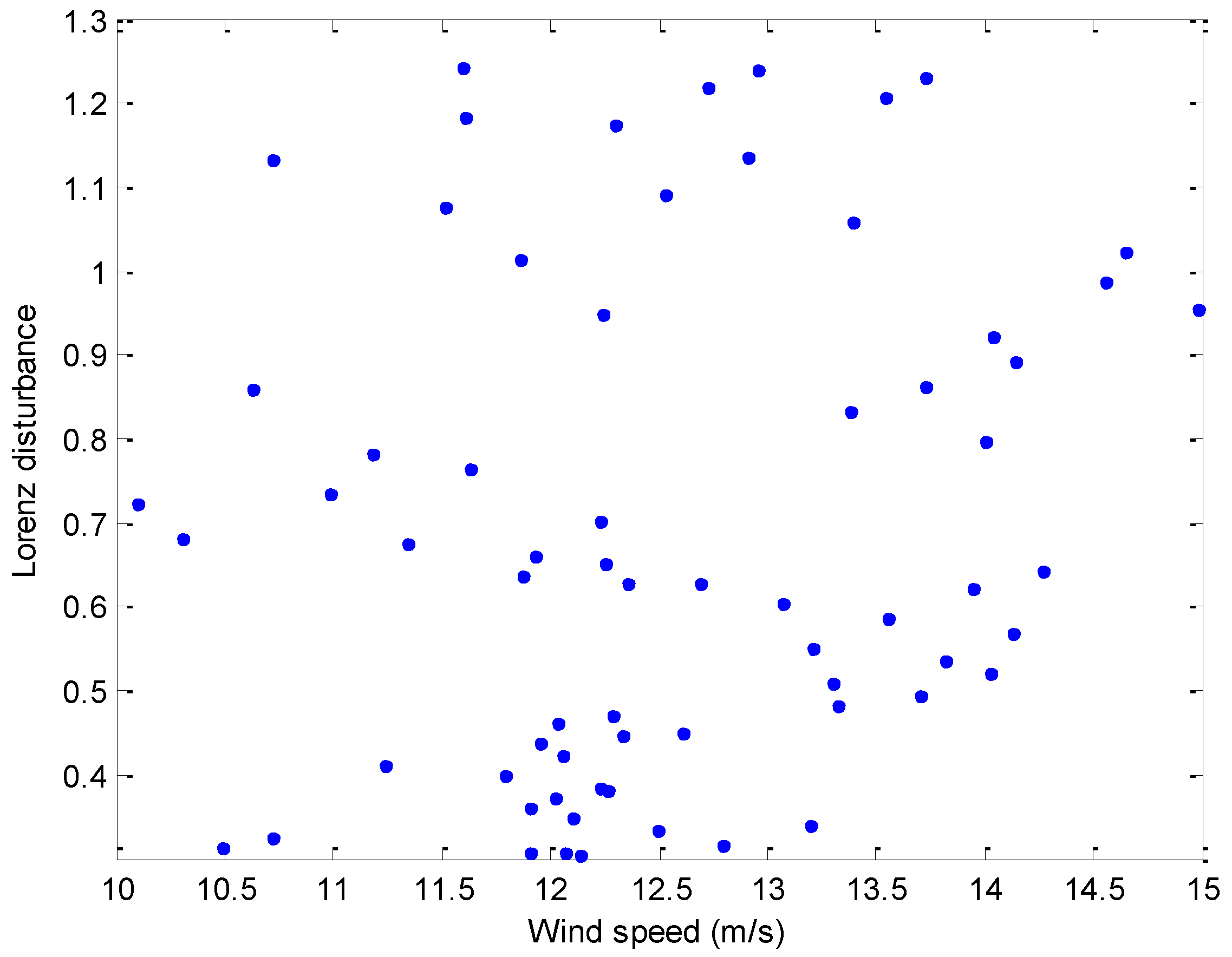
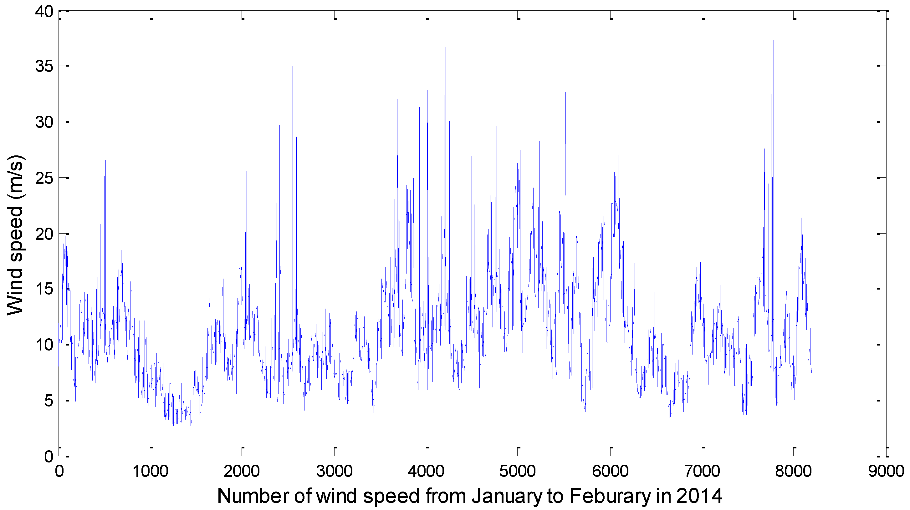
3.1. Data Description

3.2. Error Criteria
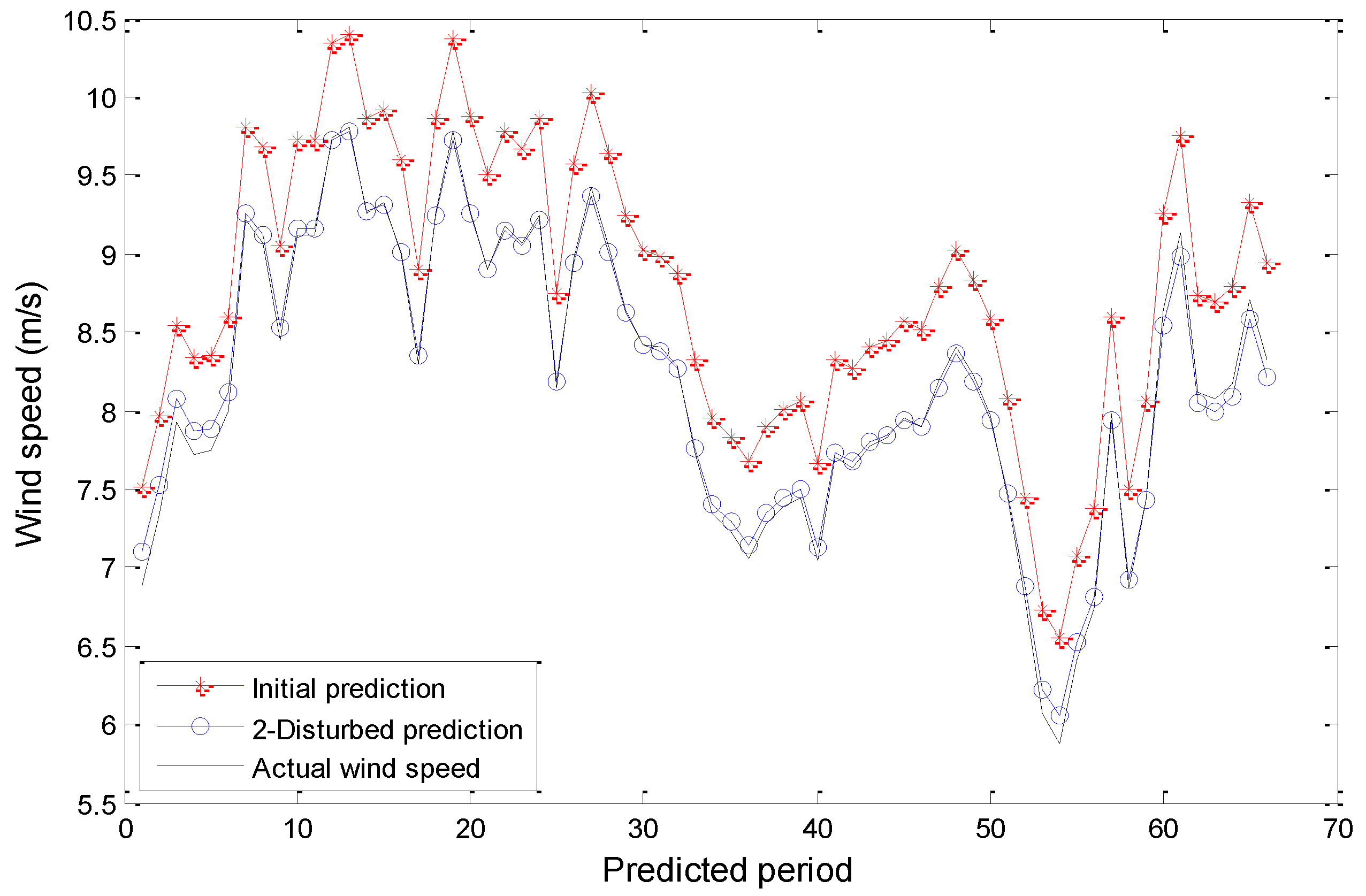
3.3. Wind Disturbance model When Rayleigh Number Equals to 45
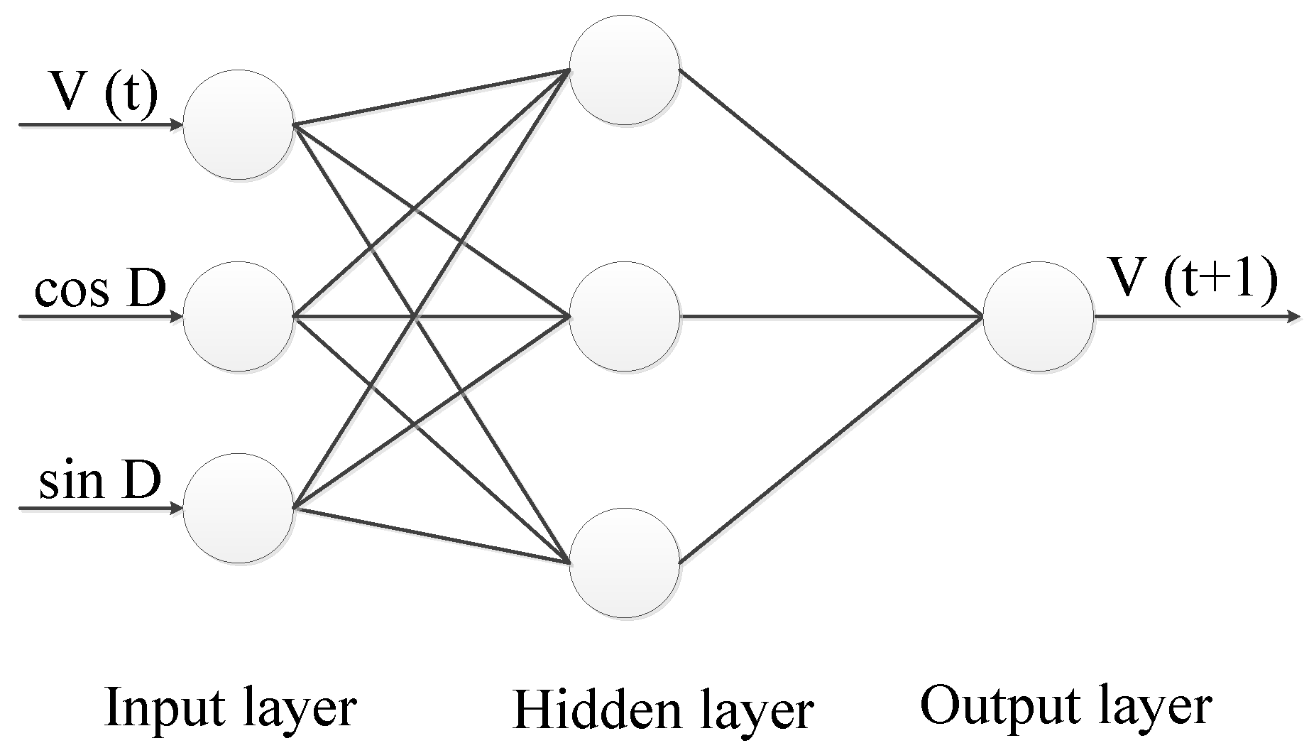
3.3.1. BP Neural Network

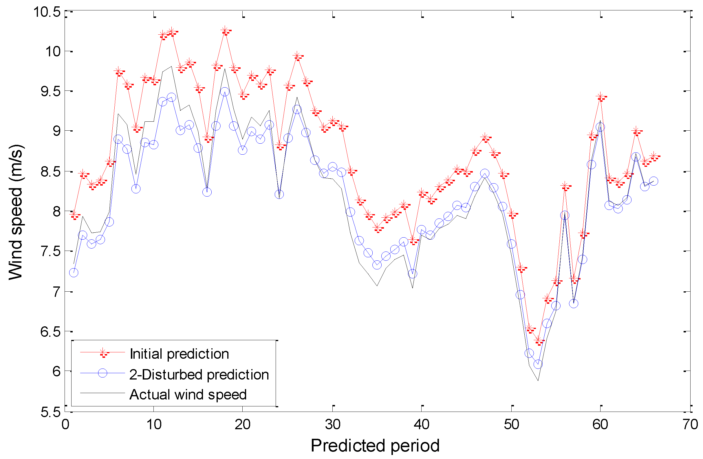
3.3.2. Modeling Process and Discussion
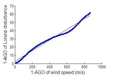
| Polynomial Expression | Accumulated Generating Model | Fitting Error (RMSE) |
|---|---|---|
| f (x) = p1 · x + p2 p1 = 0.0648, p2 = 2.6455 |  | 2.218 |
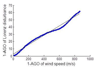
| f (x) = p1 · x2 + p2 · x + p3 p1 = −1.0713 × 10⁻⁶, p2 = 0.0657 p3 = 2.5099 |  | 2.234 |
| f (x) = p1 · x3 + p2 · x2 + p3 · x + p4 p1 = 1.672 × 10⁻⁷, p2 = −0.0002 p3 = 0.1430, p3 = −3.2818 |  | 0.8353 |
| f (x) = p1 · x4 + p2 · x3 + p3 · x2 + p4 · x + p5 p1 = 9.1690 × 10⁻¹¹, p2 = 6.0698 × 10⁻⁹ p3 = −1.2911 × 10⁻⁴, p4 = 0.1248 p5 = −2.4246 |  | 0.8027 |
| f (x) = p1 · x5 + p2 · x4 + p3 · x3 + p4 · x2 + p5 · x + p6 p1 = −1.1187 × 10⁻¹², p2 = 2.5436 × 10⁻⁹ p3 = −1.9104 × 10⁻⁶, p4 = 5.0681 × 10⁻⁴ p5 = 0.0429, p6 = 0.2498 |  | 0.4496 |
| Degree of Polynomial | Wind Forecasting Error | |||
|---|---|---|---|---|
| MAE (I) (m/s) | MAE (m/s) | RMSE (I) (m/s) | RMSE (m/s) | |
| 1 | 0.5772 | 0.0729 | 0.5870 | 0.0979 |
| 2 | 0.5935 | 0.0535 | 0.5989 | 0.0789 |
| 3 | 0.6632 | 0.2230 | 0.6720 | 0.2672 |
| 4 | 0.6248 | 0.1897 | 0.6365 | 0.2267 |
| 5 | 0.4377 | 0.1643 | 0.4683 | 0.2268 |
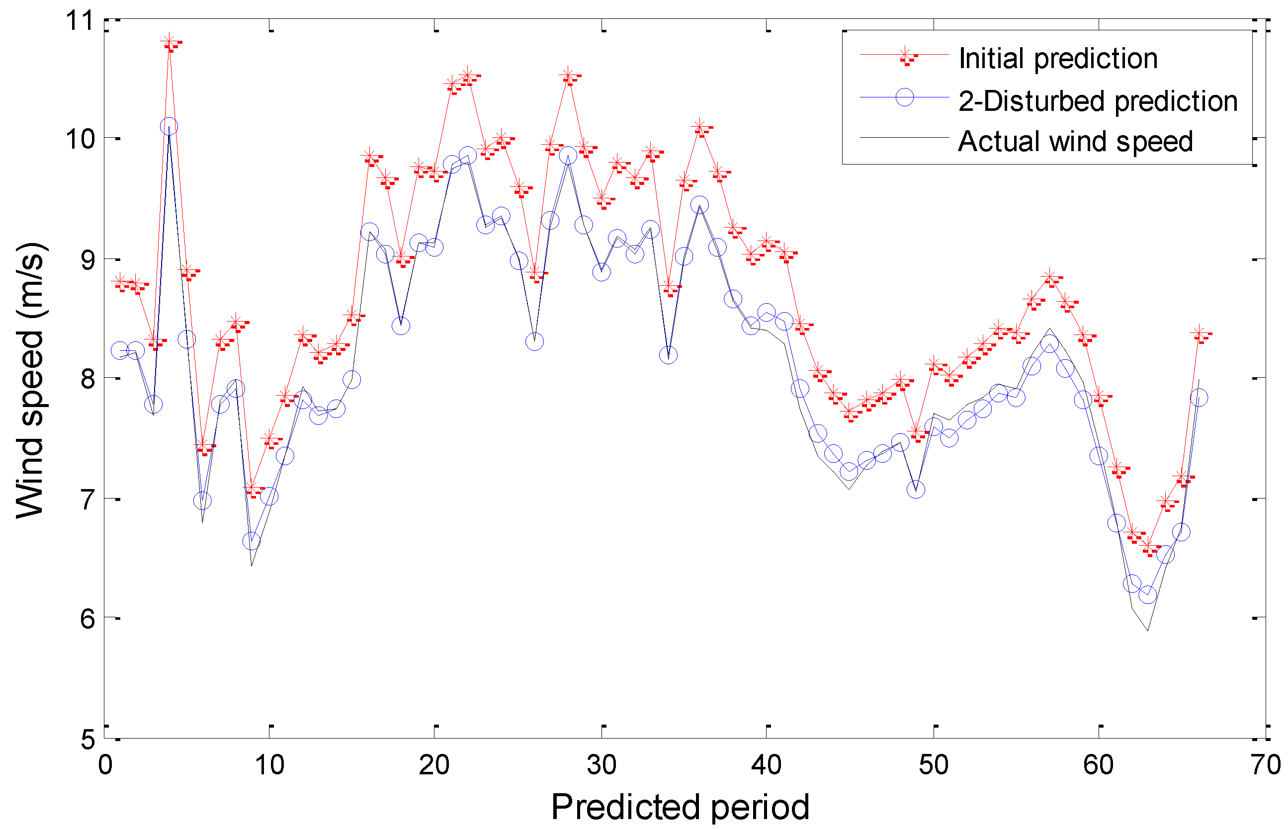
3.4. Wind Disturbance Models When Rayleigh Numbers are Equal to 0.7, 12, and 16, Respectively
| Rayleigh Number | Polynomial Expression | Accumulated Generating Model | Error (RMSE) |
|---|---|---|---|
| 0.7 | f (x) = p1 · x2 + p2 · x + p3 p1 = −4.8249 × 10⁻⁵, p2 = 0.0919 p3 = 2.3845 |  | 0.7586 |
| 12 | f (x) = p1 · x + p2 p1 = 0.0888, p2 = 5.1913 |  | 4.125 |
| 16 | f (x) = p1 · x2 + p2 · x + p3 p1 = 2.2630 × 10⁻⁵, p2 = 0.0542 p3 = 7.8821 |  | 2.746 |
| 45 | f (x) = p1 · x2 + p2 · x + p3 p1 = −1.0713 × 10⁻⁶, p2 = 0.0657 p3 = 2.5099 |  | 2.234 |
| Rayleigh Number | Wind Forecasting Error | |||||
|---|---|---|---|---|---|---|
| MAE (I) (m/s) | MAE (m/s) | MAE (P) (m/s) | RMSE (I) (m/s) | RMSE (m/s) | RMSE (P) (m/s) | |
| 0.7 | 0.5278 | 0.1447 | 0.4047 | 0.5429 | 0.1720 | 0.5201 |
| 12 | 0.7690 | 0.1397 | 0.7185 | 0.8035 | 0.1903 | 0.9870 |
| 16 | 0.6137 | 0.0581 | 0.4108 | 0.6139 | 0.0769 | 0.5230 |
| 45 | 0.5935 | 0.0535 | 0.4650 | 0.5989 | 0.0789 | 0.6486 |


4. Conclusions
Acknowledgments
Author Contributions
Conflicts of Interest
References
- Cheng, M.; Zhu, Y. The state of the art of wind energy conversion systems and technologies: A review. Energy Convers. Manag. 2014, 88, 332–347. [Google Scholar] [CrossRef]
- Irwanto, M.; Gomesh, N.; Mamat, M.R.; Yusoff, Y.M. Assessment of wind power generation potential in Perlis, Malaysia. Renew. Sustain. Energy Rev. 2014, 38, 296–308. [Google Scholar] [CrossRef]
- Global Wind Energy Council (GWEC). Available online: http://www.gwec.net/global-figures/graphs/ (accessed on 12 June 2014).
- Jung, J.; Broadwater, R.P. Current status and future advances for wind speed and power forecasting. Renew. Sustain. Energy Rev. 2014, 31, 762–777. [Google Scholar] [CrossRef]
- Fan, C.; Liu, S. Wind speed forecasting method: Grey related weighted combination with revised parameter. Energy Proced. 2011, 5, 550–554. [Google Scholar] [CrossRef]
- Chandel, S.S.; Ramasamy, P.; Murthy, K.S.R. Wind power potential assessment of 12 locations in western Himalayan region of India. Renew. Sustain. Energy Rev. 2014, 39, 530–545. [Google Scholar] [CrossRef]
- Rasheed, A.; Kristoffer Suld, J.; Kvamsdal, T. A multiscale wind and power forecast system for wind farms. Energy Proced. 2014, 53, 290–299. [Google Scholar] [CrossRef]
- Peng, H.; Liu, F.; Yang, X. A hybrid strategy of short term wind power prediction. Renew. Energy 2013, 50, 590–595. [Google Scholar] [CrossRef]
- Yesilbudaka, M.; Sagiroglub, S.; Colakc, I. A new approach to very short term wind speed prediction using k-nearest neighbor classification. Energy Convers. Manag. 2013, 69, 77–86. [Google Scholar] [CrossRef]
- Sfetsos, A. A comparison of various forecasting techniques applied to mean hourly wind speed time series. Renew. Energy 2000, 21, 23–35. [Google Scholar] [CrossRef]
- Jin, X.; Zhang, Z.; Shi, X.; Ju, W. A review on wind power industry and corresponding insurance market in China: Current status and challenges. Renew. Sustain. Energy Rev. 2014, 38, 1069–1082. [Google Scholar] [CrossRef]
- Su, Z.; Wang, J.; Lu, H.; Zhao, G. A new hybrid model optimized by an intelligent optimization algorithm for wind speed forecasting. Energy Convers. Manag. 2014, 85, 443–452. [Google Scholar] [CrossRef]
- Wang, J.; Zhang, W.; Li, Y.; Wang, J.; Dang, Z. Forecasting wind speed using empirical mode decomposition and Elman neural network. Appl. Soft Comput. 2014, 23, 452–459. [Google Scholar] [CrossRef]
- An, S.; Shi, H.; Hu, Q.; Li, X.; Dang, J. Fuzzy rough regression with application to wind speed prediction. Inf. Sci. 2014, 282, 388–400. [Google Scholar] [CrossRef]
- Sheela, K.G.; Deepa, S.N. Neural network based hybrid computing model for wind speed prediction. Neurocomputing 2013, 122, 425–429. [Google Scholar] [CrossRef]
- Liu, B.Z.; Peng, J.H. Nonlinear Dynamics, 1st ed.; Higher Education Press: Beijing, China, 2007; pp. 120–143. [Google Scholar]
- Saltzman, B. Finite amplitude free convection as an initial value problem-I. J. Atmos. Sci. 1962, 19, 329–341. [Google Scholar] [CrossRef]
- Lorenz, E.N. Deterministic nonperiodic flow. J. Atmos. Sci. 1963, 20, 130–141. [Google Scholar] [CrossRef]
- Lorenz, E.N. The Essence of Chaos, 1st ed.; China Meteorological Press: Beijing, China, 1997; pp. 127–137. [Google Scholar]
- Wang, Q.; Huang, W.; Feng, J. Multiple limit cycles and centers on center manifolds for Lorenz system. Appl. Math. Comput. 2014, 238, 281–288. [Google Scholar] [CrossRef]
- Algaba, A.; Fernández-Sánchez, F.; Merino, M.; Rodríguez-Luis, A.J. Centers on center manifolds in the Lorenz, Chen and Lü systems. Commun. Nonlinear Sci. Numer. Simul. 2014, 19, 772–775. [Google Scholar] [CrossRef]
- Rayleigh, L. On convective currents in a horizontal layer of fluid, when the higher temperature is on the underside. Philos. Mag. Ser. 1916, 32, 529–546. [Google Scholar] [CrossRef]
- Deng, J.L. The primary Methods of Grey System Theory, 2nd ed.; Huazhong University of Science and Technology Press: Wuhan, China, 2005; pp. 27–55. [Google Scholar]
- Deng, J.L. Grey Prediction and Grey Decision Making, 1st ed.; Huazhong University of Science and Technology Press: Wuhan, China, 2002; pp. 45–71. [Google Scholar]
- Wang, X.; Qi, L.; Chen, C.; Tang, J.; Jiang, M. Grey system theory based prediction for topic trend on Internet. Eng. Appl. Artif. Intell. 2014, 29, 191–200. [Google Scholar] [CrossRef]
- Bahrami, S.; Hooshmand, R.-A.; Parastegari, M. Short term electric load forecasting by wavelet transform and grey model improved by PSO (particle swarm optimization) algorithm. Energy 2014, 72, 434–442. [Google Scholar] [CrossRef]
- Wang, X.; Li, H. Multiscale prediction of wind speed and output power for the wind farm. J. Control Theory Appl. 2012, 10, 251–258. [Google Scholar] [CrossRef]
- Hu, J.; Wang, J.; Zeng, G. A hybrid forecasting approach applied to wind speed time series. Renew. Energy 2013, 60, 185–194. [Google Scholar] [CrossRef]
- Shi, J.; Guo, J.; Zheng, S. Evaluation of hybrid forecasting approaches for wind speed and power generation time series. Renew. Sustain. Energy Rev. 2012, 16, 3471–3480. [Google Scholar] [CrossRef]
- Zhao, X.; Wang, S.; Li, T. Review of evaluation criteria and main methods of wind power forecasting. Energy Proced. 2011, 12, 761–769. [Google Scholar] [CrossRef]
- Wang, J.; Sheng, Z.; Zhou, B.; Zhou, S. Lightning potential forecast over Nanjing with denoised sounding-derived indices based on SSA and CS-BP neural network. Atmos. Res. 2014, 137, 245–256. [Google Scholar] [CrossRef]
- Ren, C.; An, N.; Wang, J.; Li, L.; Hu, B.; Shang, D. Optimal parameters selection for BP neural network based on particle swarm optimization: A case study of wind speed forecasting. Knowl.-Based Syst. 2014, 56, 226–239. [Google Scholar] [CrossRef]
- Yu, F.; Xu, X. A short-term load forecasting model of natural gas based on optimized genetic algorithm and improved BP neural network. Appl. Energy 2014, 134, 102–113. [Google Scholar] [CrossRef]
- Palomares-Salas, J.C.; Agüera-Pérez, A.; González de la Rosa, J.J.; Moreno-Muñoz, A. A novel neural network method for wind speed forecasting using exogenous measurements from agriculture stations. Measurement 2014, 55, 295–304. [Google Scholar] [CrossRef]
- Wu, W.-Y.; Chen, S.-P. A prediction method using the grey model GMC(1,n) combined with the grey relational analysis: A case study on Internet access population forecast. Appl. Math. Comput. 2005, 169, 198–217. [Google Scholar] [CrossRef]
- Hamzacebi, C.; Es, H.A. Forecasting the annual electricity consumption of Turkey using an optimized grey model. Energy 2014, 70, 165–171. [Google Scholar] [CrossRef]
© 2014 by the authors; licensee MDPI, Basel, Switzerland. This article is an open access article distributed under the terms and conditions of the Creative Commons Attribution license (http://creativecommons.org/licenses/by/4.0/).
Share and Cite
Zhang, Y.; Yang, J.; Wang, K.; Wang, Y. Lorenz Wind Disturbance Model Based on Grey Generated Components. Energies 2014, 7, 7178-7193. https://doi.org/10.3390/en7117178
Zhang Y, Yang J, Wang K, Wang Y. Lorenz Wind Disturbance Model Based on Grey Generated Components. Energies. 2014; 7(11):7178-7193. https://doi.org/10.3390/en7117178
Chicago/Turabian StyleZhang, Yagang, Jingyun Yang, Kangcheng Wang, and Yinding Wang. 2014. "Lorenz Wind Disturbance Model Based on Grey Generated Components" Energies 7, no. 11: 7178-7193. https://doi.org/10.3390/en7117178