High Performance Reduced Order Models for Wind Turbines with Full-Scale Converters Applied on Grid Interconnection Studies


Abstract
: Wind power has achieved technological evolution, and Grid Code (GC) requirements forced wind industry consolidation in the last three decades. However, more studies are necessary to understand how the dynamics inherent in this energy source interact with the power system. Traditional energy production usually contains few high power unit generators; however, Wind Power Plants (WPPs) consist of dozens or hundreds of low-power units. Time domain simulations of WPPs may take too much time if detailed models are considered in such studies. This work discusses reduced order models used in interconnection studies of synchronous machines with full converter technology. The performance of all models is evaluated based on time domain simulations in the Simulink/MATLAB environment. A detailed model is described, and four reduced order models are compared using the performance index, Normalized Integral of Absolute Error (NIAE). Models are analyzed during wind speed variations and balanced voltage dip. During faults, WPPs must be able to supply reactive power to the grid, and this characteristic is analyzed. Using the proposed performance index, it is possible to conclude if a reduced order model is suitable to represent the WPPs dynamics on grid studies.1. Introduction
Various topologies of Wind Turbine Generators (WTGs) have come up during the last three decades, and different solutions for grid interconnection have been presented in the market. Connection of a new Wind Power Plant (WPP) to a power system needs to be approved by the Transmission System Operator (TSO), and preliminary studies are performed with a focus on the WPP’s impact on the grid. These studies are supported by mathematical models, which need to reproduce with accuracy the WTG behavior during some regular power system phenomena.
Nowadays, WPP modeling for grid interconnection studies is an important issue, owing to the significant increase in grid-connected wind power capacity around the world [1,2]. WPPs can have tens to hundreds of WTGs, which is a large number when compared to conventional generation plants. Modeling each of these WTGs separately increases the complexity and compromises simulation processing time significantly [1]. Moreover, there are fundamental differences between conventional plants and WPPs in terms of prime mover control, generator size and the power electronics used in some WTG topologies [3].
WTG dynamic models have been developed to study the WPP impacts on the power system. These models have been applied for transient stability studies in wind speed variations [3–6], voltage ride-through capability [1,3,5,7,8], reactive power compensation [7], frequency support capability [9–11] and for steady-state studies in harmonic propagation [12,13] and load flow analysis [14].
Customized models used to integration studies need to be able to reduce the processing time [2,15], keeping the main WPP dynamic behavior. Thus, the impact of a power system transient on the WPP and that of the WPP on the power system can be evaluated [16,17].
Many Grid Codes (GCs) require dynamic models able to represent with accuracy the dynamic behavior of a WTG when connected to a power system. These GC requirements have led to the development of many dynamic models by wind turbine manufacturers [2]. The first generation of generic models developed for use in grid interconnection studies had detailed models [7].
The second generation of models must be able to simulate new GCs requirements. Voltage ride-through capability is the phenomenon most studied by manufacturers and in academia, because GC specifications require WTGs to be able to ride through grid disturbances, which bring down voltages to very low levels [1]. Other requirements, such as reactive power control and frequency support, have a longer duration than voltage ride through, and models need to be adapted to long-time simulation with slow dynamics.
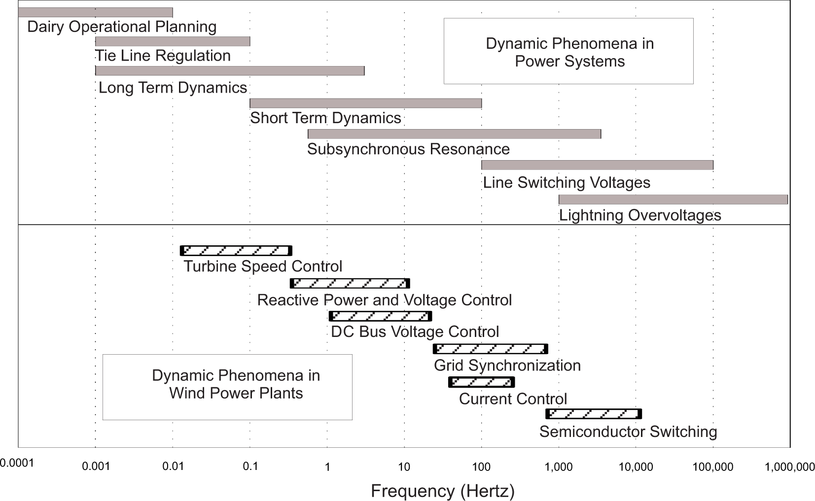
Figure 1 shows the most regular power system dynamic phenomena in terms of frequency range. Some power system dynamics are correlated with WTG controllers, i.e., in a subsynchronous resonance study, the reactive power control has a large influence, while the semiconductor switching dynamic does not affect this type of study and can be neglected from the model. The computer simulations should be defined properly to guarantee sufficient model accuracy for the studied phenomena and ensure that simulations provide adequate results [18].
The paper is subdivided into the following sections. Section 2 presents a general discussion about mathematical models and presents the methodology used to develop the detailed and reduced order models in the time domain. Section 3 introduces the performance index used to compare the models. Section 4 shows case studies and a comparison between the detailed and reduced order models. Conclusions are stated in Section 5.
2. Synchronous Generator with Full-Scale Converter Models
Mathematical models of WTGs are required for power system studies by utilities and system operators [14], and they can be developed in the time domain or the frequency domain. Time domain simulations are normally processed in commercial software packages. However, with an increasing number of buses and generators, time domain simulations may take too much processing time. As simulation results are presented in the time domain, mathematical techniques for harmonic analysis are necessary. Frequency domain analysis is a fast tool that takes almost the same time to process, independent of the number of WTGs considered. Its fast performance is due to the computation through matrices [13].
A Real-Time Discrete Simulator (RTDS) is a device that is used to reduce simulation time considerably. While in commercial software packages, such as MATLAB (MathWorks, Natick, MA, USA), Power Factory (DigSilent, Gomaringen, Germany), Electromagnetic Transients Program (EMTP) and others, a simulation of a WPP with 50 generators during 10 s can demand many hours of computer processing, the same simulation on an RTDS will take only 10 s. Another advantage of real-time simulators is their capability to communicate with hardware, allowing design, testing and validation under operational conditions before being placed in the field [19]. The main drawback of RTDS devices is their cost, which is much higher than personal computers.
WPPs using synchronous generators operating at variable speed came on the market as an attractive alternative to eliminate the mechanical gearbox. Connected to the grid by means of frequency converters, these machines can operate at low rotational speed due to a large amount of magnetic poles in the generator. The highlights of this technology are fault ride-through capability during network disturbances and the ability to extract maximum power from wind due to its variable speed operation [8,13]. In addition, new GC requirements aid the increased use of this topology as the most interesting solution.
2.1. Detailed Model
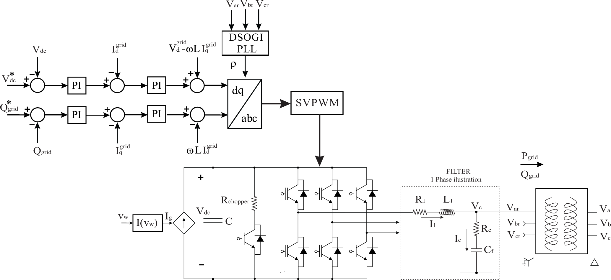
In this work, a detailed model is considered as the base case. Based on this detailed model, four reduced order models are developed and compared with it. The main parts of the detailed model are shown in Figure 2 and are detailed in the next sections.
2.1.1. Wind Energy Extraction
Wind energy extraction is possible using blades connected to the nacelle. In the last three decades, the design of blades has been developing quickly, mainly with the use of new materials, which allow constructing blades of tens of meters and with low solidity. Blades turn a shaft, which is connected to the generator directly or through a gearbox. WTGs with full-scale converters and a high number of poles have removed the gearbox to reduce maintenance costs, which is an important factor in offshore applications.
According to WTG characteristics, a mechanical power analytic function can be defined as Equation (1). Cp is a nonlinear performance coefficient and depends on the turbine characteristics [4,20,21]. In this work, Equations (2)–(4) are adopted.
A wind turbine swept area;
R turbine radius;
Vw wind speed;
ωt turbine rotational speed;
ρ air density;
λ tip speed ratio;
β blade pitch angle.
2.1.2. Synchronous Generator Model
In this work, a wound rotor synchronous machine model is used. Other generator types, such as permanent magnet synchronous generators or squirrel-cage asynchronous generators, can be easily used with the methodology introduced in this work, since the stator windings are connected to the grid through a full-scale power converter.
The wound rotor synchronous machine model used is modeled in the d-q (direct-quadrature) rotor reference frame, as given in [22]. Two damping windings and one field winding are considered, representing sub-transient and transient phenomena, respectively. The damping windings are not considered in some works, because a synchronous machine is current-controlled [5,23], but these windings are considered in this work in order to compare reduced order models with a detailed model.
In synchronous machine topologies with a diode rectifier, the DC (Direct Current) bus voltage can be controlled by the machine field excitation system. The modeling of this control considers the delay caused by the thyristors, the field and damping winding time constants. Two Proportional-Integral (PI) controllers can be used, where the outer DC voltage loop gives a reference to an inner current loop that controls the voltage applied in the field winding [24]. In this work, the field voltage is assumed to be constant, because during voltage dip, the machine is decoupled from the grid and, also, wind speed is considered with slow variations.
2.1.3. Machine-Side Control (MSC) and Grid-Side Control (GSC)
Machine-Side Control (MSC) is designed with the objective of maximizing power extraction and limiting WTG braking power [25]. In this work, the power injection into the DC bus is optimized based on wind speed. Grid-Side Control (GSC) is designed to keep the DC bus voltage constant and to control reactive power injection into the grid. Both MSC and GSC have inner loops with current controllers. Proportional-Integral (PI) controllers, as given in Equation (5), are used in all inner and outer control loops.
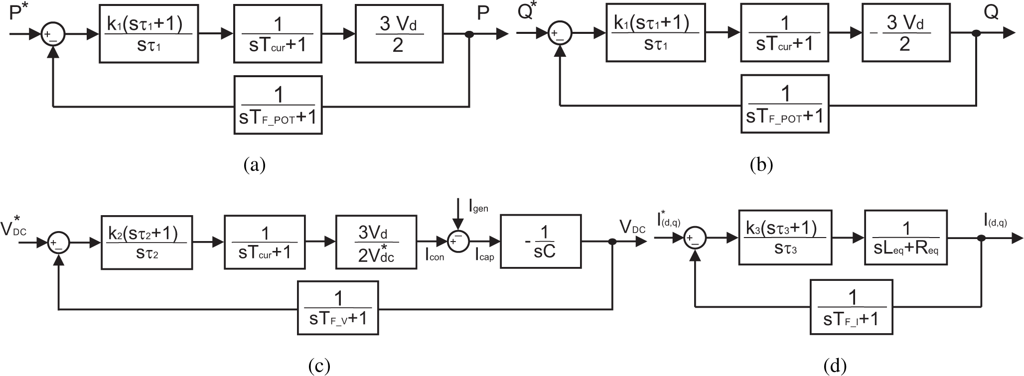
The methodology for tuning the controllers gains for the detailed model is the same used in the reduced order models. In outer loop design, the inner loop was considered ideal (Tcur = 0). The design of active and reactive power control is based on the opened-loop transfer function, as shown in Figure 3a,b, respectively. Canceling the pole from the opened-loop transfer function with τ1 = TFPOT and using the closed-loop transfer function, a pole is allocated in a frequency fC, smaller than the inner loop frequency (generally between five- and ten-times smaller), using gains calculated by Equation (6).
The voltage control loop gains, as shown in Figure 3c, are more complex due to a pole at the origin. Considering the closed-loop transfer function without the measurement filter effect (TFV = 0), two frequencies (ωC1 and ωC2) are defined, where gains can be calculated by Equations (7) and (8).
Gains of all inner loops are designed based on Figure 3d. Using the opened-loop transfer function, the plant pole can be canceled when τ3 = Leq/Req. The closed-loop transfer function can be written in canonical form. Thus, using the damping factor equal to to provide good dynamic performance [26], the current loop PI gains can be calculated by Equation (9).
2.1.4. Phase-Locked Loop
An important issue in the connection of WPPs to the grid is the synchronization system, since the control of the power factor is done in these systems and requires accurate phase information of utility voltages [26]. Phase-locked loop (PLL) is the most common structure used to calculate grid phase. The designed PLL should be robust enough to reject disturbances, such as voltage dips, unbalances and harmonics [27].
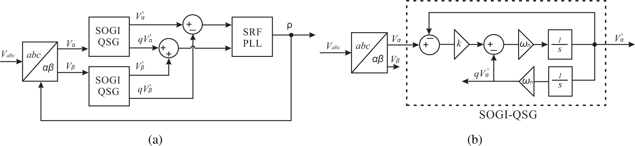
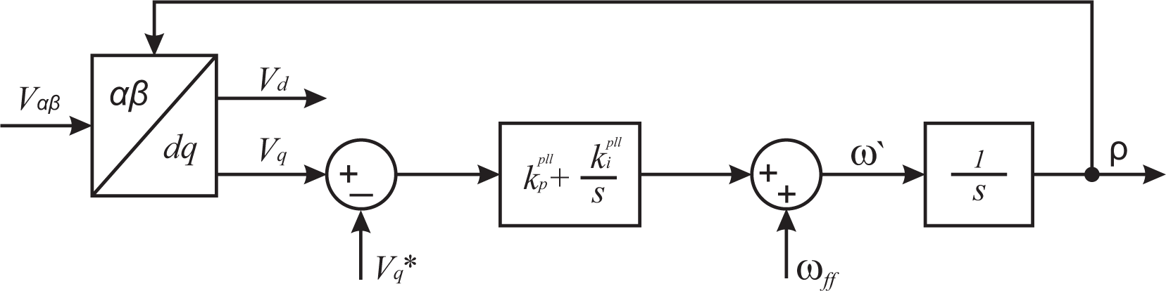
This work uses Dual Second Order Generalized Integrator PLL (DSOGI-PLL), which has two Second Order Generalized Integrators (SOGIs) with a Quadrature Signal Generator (QSG) to separate the positive and negative sequence of the grid voltage and a Synchronous Reference Frame (SRF) structure to estimate angular position, as shown in Figure 4a.
The SOGI structure has a filter characteristic, and it generates signals in quadrature, as shown in Figure 4b. These signals are used in a stationary αβ positive sequence detector.
The transfer functions of an SOGI are given by Equation (10).
ωn rated grid frequency;
k SOGI gain.
A critically damped response is achieved when [28]. This gain value results in an interesting selection in terms of good dynamic response and limiting overshoot.
The SRF-PLL configuration is shown in Figure 5. Grid voltages in the αβ reference frame are transformed to the d-q synchronous reference frame using Park’s transformation. The angular position of this d-q reference frame is controlled by a feedback loop, which regulates the q-component of the voltage to zero [29]. For a balanced system, grid voltages in the direct and quadrature axis can be written as Equation (11).
voltage peak;
ρ angle of synchronous system calculated by PLL.
θ0 phase angle of the fundamental component of grid voltage.
Note that and vq = 0 when ρ = ωt + θ0. The controller is thus designed to have vq equal zero in steady state. Analyzing Figure 5, it is possible to write Equation (12).
ωff grid frequency feedforward.
Replacing Equation (11) into Equation (12), disregarding the feedforward effect ωff, results in Equation (14), which is a synchronization structure with a non-linear dynamic.
This equation can be linearized considering ρ(t) ≈ ωt + θ0 and sin(γ) ≈ γ for γ ≈ 0. Thus, a closed-loop system, with transfer function H(s), is given by Equation (15).
Substituting Equation (13) into Equation (15), Equation (16) is obtained.
The values of damping ξ and frequency ωm are adjusted in a PLL tuning process. A good compromise between dynamic performance and filtering are obtained with and ωm = 100 rad/s, and these values were used in this work.
2.1.5. LCL Filter
The LCL filter is used to reduce harmonics generated due to inverter switching [30]. The inductance L1, as shown in Figure 2, is calculated according to the maximum current ripple iripple and can be obtained by Equation (18) [31].
The capacitor value is limited by the decrease of the power factor at rated power (generally less than 5%). After this, the filter resonance frequency needs to be analyzed and should lie in a range between ten-times the line frequency and one-half of the switching frequency (10fn ≤ fres ≤ 0.5fs). In this work, the transformer linkage inductance forms the second filter inductance Lf. To reduce the resonant peak, a resistor is connected in series with the capacitor, whose value is chosen as one-third of the capacitor impedance at the resonant frequency [30].
2.1.6. DC Bus Protection
During voltage dips, the generated power injection into the grid is limited by inverter capacity. For this reason, the difference between produced and injected power charges the DC bus capacitor; thus, many topologies use a protection chopper that dissipates this energy in the DC bus [1]. In this work, the chopper is activated when the DC voltage is higher than 5% of the nominal value.
2.2. First Reduced Order Model: DC Current Source Model
This model is based on the idea that from the Point of Common Coupling (PCC), the machine performance is not relevant, because it is decoupled from the grid by a power converter [7]. Therefore, the drive train model, synchronous machine and machine-side converter can be omitted. A DC current source, controlled by wind speed, is used to represent the generator current injection [1], as shown in Figure 6. From the grid side, all components and controllers are the same as those used in the detailed model.
2.3. Second Reduced Order Model: Average Value Model
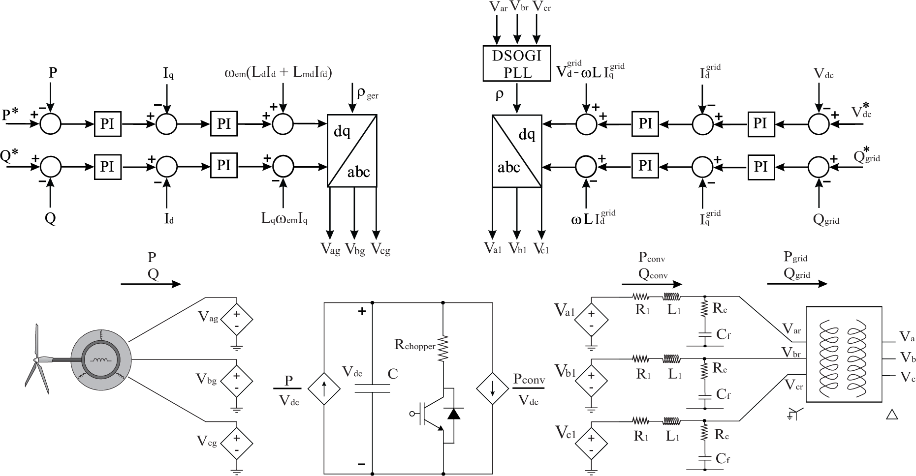
The main limitation in increasing the simulation step size is the converter switching frequency, generally in the order of kilohertz (1–5 kHz), requiring a simulation step size of microseconds (10–50 μs). Thus, in WPP interconnection studies, which require only the fundamental frequency, an average value model can be used. This model is shown in Figure 7, where three phase converters are substituted by ideal voltage sources. In this structure, the calculated controller voltage is applied directly in voltage sources, without a Pulse Width Modulation (PWM) structure. The average model can be simulated using a simulation step size ten-times bigger than the detailed model, significantly decreasing the simulation processing time.
2.4. Third Reduced Order Model: Alternating Current (AC) Ideal Voltage Source Model
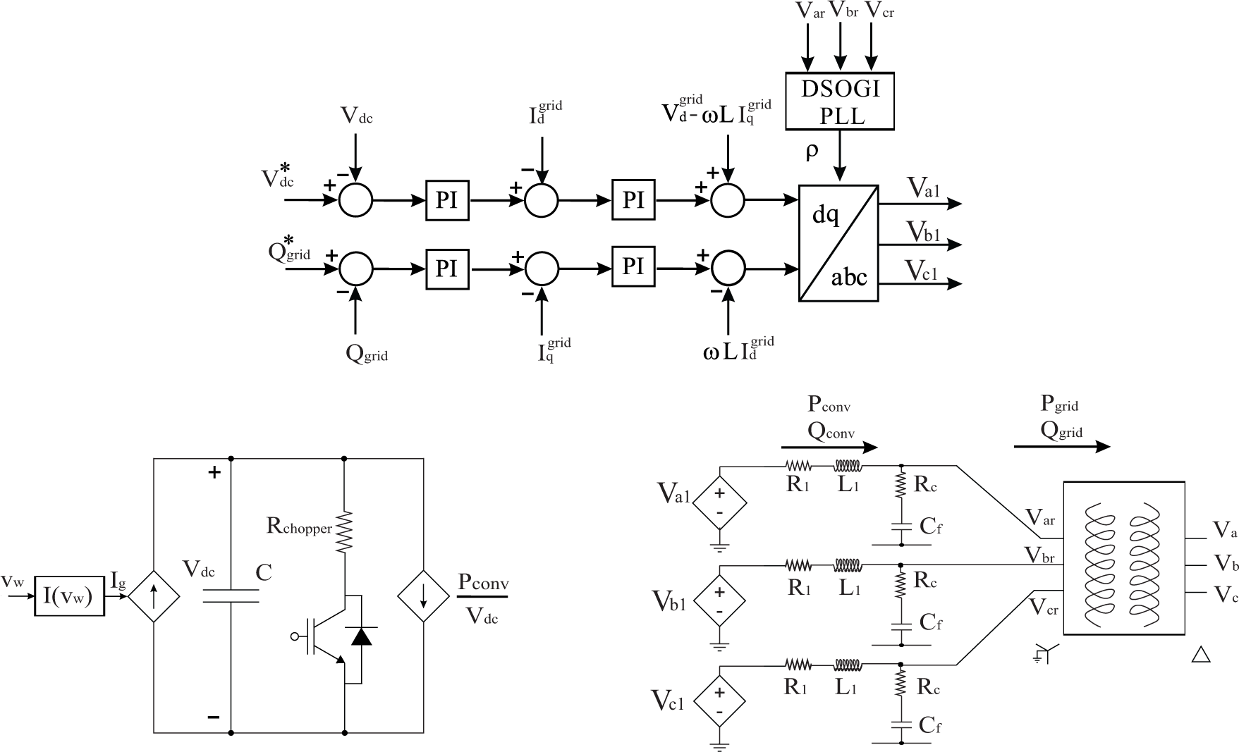
The Alternating Current (AC) Voltage Source Model is based on the average model and the DC current source model introduced previously, where the first one omits the generator and rectifier converter and the second one considers only fundamental frequency. With these characteristics, a model is designed as shown in Figure 8. The simulation step size has the same order as that of the average value model, but with a reduced number of components, thereby reducing the processing time.
2.5. Fourth Reduced Order Model: AC Ideal Current Source Model
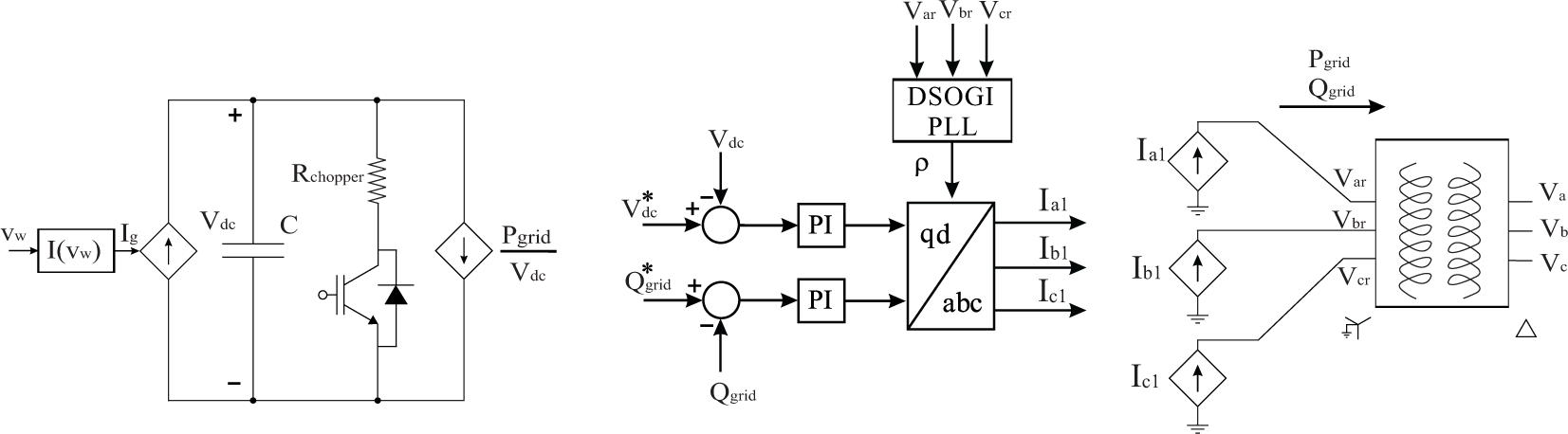
The AC Current Source has a similar model simplification as presented in the AC voltage source model, but eliminating the inner loop control (current loop). In some WPP interconnection studies, the dynamics involved in the inner loop can be disregarded. This way, outer loop controllers are responsible for calculating the current injection into the grid through current sources. In this model, the LCL filter is eliminated, because the currents calculated by the controllers are grid currents, as shown in Figure 9. In this model, it is possible to perform simulation with a step size one hundred-times greater than the detailed model, considerably reducing the simulation processing time.
3. Performance Index
A simplified model that replaces a more detailed model presents good accuracy in the simulation results, preserving the relevant WPP dynamics. A successful simplified model will reduce the simulation time without significantly compromising on the accuracy of the results in comparison to the detailed model [1,19].
The way of determining the accuracy of a model is an important topic that needs to be explored more. Many works conclude that a model is adequate using qualitative analysis, such as:
A good match between the wind turbine vendor model and the adjusted generic model [7];
Only relatively small discrepancies between simulated and measured behavior [18];
The response of the models to a measured wind-speed sequence is compared with measurements, and an acceptable degree of correspondence can be observed [20];
The model developed performs satisfactorily for slow dynamics when compared with the results obtained from simulation, considering the detailed model [6].
This work proposes the use of a performance index to ensure that a model provides a realistic and robust assessment of the studied phenomena. This is a quantitative way of standardizing the model accuracy, avoiding mismatches between analysis, helping in the identification of model limitations and realizing implementation improvements.
Several performance indexes have been proposed for use in connection with the design and optimization of linear automatic control systems [32]. The Integral of Squared Error (ISE), Equation (19), and the Integral of Absolute Error (IAE), Equation (20), are two performance indexes used in control parameter tuning. ISE penalizes large differences between models. On the other hand, IAE does not add weight to any of the differences, and it measures the area between two curves.
VRef variable from the reference model;
VRed variable from the reduced order model.
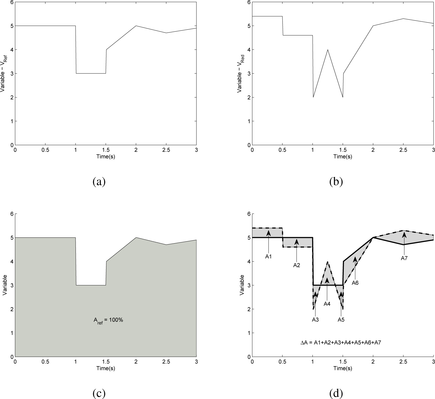
In fact, the area between curves is directly related to the difference between them. Assume a reference model, defined as Model 1, having a variable VRef, with dynamic characteristics, as shown in Figure 10a, and a reduced order model, defined as Model 2, which has a variable VRed, with different dynamic characteristic, as shown in Figure 10b. The area from the VRef curve is defined as 100%, as shown in Figure 10c, and differences between the VRef area and VRed area are represented by the sum of areas, as shown in Figure 10d.
Defining the performance index to compare models as the sum of areas between curves (∆A) divided by the area from Model 1 (Aref) is the same as IAE normalized. Thus, the Normalized Integral of Absolute Error (NIAE), as given by Equation (21), can be used to calculate the similarity between the detailed model and the reduced order model.
The process of defining a value for NIAE, where one model can be considered adequate to represent the dynamic plant response, will depend on some criteria. The best model can be defined as being able to reproduce the same result as measured in a WTG and have NIAE equal two one. However, there are many inherent errors associated with a measurement system, such as [7]:
Current and potential transformers tolerance;
Components have associated design tolerances;
Magnetic saturation and hysteresis;
Bandwidth limitations in transducers and measurement equipment.
These mismatches in the validation process permit a model to be considered adequate even with differences from the reference model. Thus, the following range of values are proposed for NIAE:
Adequate models, NIAE ≥ 0.95;
Inadequate models, NIAE < 0.95.
4. Case Studies and Simulation Results
One detailed model and four reduced order models of WTG with full-scale converters were developed in the Simulink/MATLAB environment. The simulated system consists of a transformer of 45 MVA that connects a WPP to the grid and one transformer of 2.2 MVA connected to the WTG, as shown in Figure 11. Based on the generator parameters shown in Table 1, two cases are studied to illustrate the comparison between reduced order models and the detailed model.
In what follows, the focus is on the active and reactive power at the PCC upon application of wind speed variations, as shown in Figure 12a, and balanced voltage dip, as shown in Figure 12b.
4.1. DC Current Source Model
Figure 13a shows the response of the DC current source and the detailed model when active power is injected into the grid.
The response of the first model is faster than the second, because the variation in wind speed is transmitted immediately to the DC bus. Reactive power injected into the grid is not affected by wind speed variations, as shown in Figure 13b.
The balanced voltage dip applied on the PCC causes a reduction of the active power injected into the grid, as shown in Figure 13c, and requires reactive power injection, as shown in Figure 13d. In the steady state, the active power injected by the detailed model is smaller than in the case of the reduced order model, because the generator and rectifier losses are neglected in the reduced order model. The DC current source model has NIAE for active power equal to 0.9577 during wind speed variations and NIAE equal to 0.9771 for the balanced voltage dip, as shown in Table 3, as well as a reduction of 18.71% in simulation processing time, as shown in Table 4. Thus, this model is considered adequate to represent the phenomena studied in this work and can be used in other studies with slower dynamics.
4.2. Average Value Model
The average value model presents dynamics similar to the detailed model during wind speed variations, but in the steady state, this model injects more active power than the detailed model, as shown in Figure 14a. In the reactive power, small oscillations can be observed when the wind speed changes, as shown in Figure 14b. During balanced voltage dips, the active power injected into the PCC by the average model has ripples bigger than the detailed model, as shown in Figure 14c, and the reactive power has similar dynamics, as shown in Figure 14d.
The average value model has NIAE for active power equal to 0.9758 during wind speed variations and NIAE equal to 0.9809 when the balanced voltage dip is analyzed, as shown in Table 3; thus, the average value model has a better performance than the DC Bus Current Source Model. Besides, it reduces the simulation processing time by 49.68%, as shown in Table 4.
4.3. AC Ideal Voltage Source Model
The active power injected into the grid using the AC ideal voltage source model has dynamics faster than the detailed model, as shown in Figure 15a, and a bigger value in the steady state, because the generator and converters losses are not considered. Oscillations in the reactive power during wind speed variations are not relevant, as shown in Figure 15b. During balanced voltage dips, the dynamic behavior is similar to other reduced order models with small ripples in the active power, as shown in Figure 15c, as well as the same dynamic behavior in the reactive power, as shown in Figure 15d.
The AC ideal voltage source model has NIAE for active power equal to 0.9555 during wind speed variations and NIAE equal to 0.9708 when the balanced voltage dip is analyzed, as shown in Table 3; thus, the AC ideal voltage source model has a performance similar to the DC current source model, but with the advantage of a reduction in the simulation processing time by 91.29%, as shown in Table 4.
4.4. AC Ideal Current Source Model
The AC ideal current source model is the reduced order model with the worst dynamic response. During wind speed variations, the active power injected into the grid is shown in Figure 16a, and the reactive power presents some oscillations during wind speed variations, as shown in Figure 16b. This reduced order model presents oscillations in the active power injected into the grid during balanced voltage dips, as shown in Figure 16c, and the reactive power does not have the same dynamics as the detailed model, as shown in Figure 16d.
The AC ideal current source model has NIAE for active power equal to 0.9504 during wind speed variations and NIAE equal to 0.9268 when the balanced voltage dip is analyzed, as shown in Table 3. This reduced order model can decrease the simulation processing time by 99.03%, as shown in Table 4. Based on the NIAE index, this model is considered inadequate to represent the phenomena with accuracy, such as balanced voltage dip, but it is considered adequate in wind speed variation studies or other phenomena with slower dynamics.
Table 3 consolidates the model performances based on the NIAE index. All models are considered adequate to represent transient behavior during wind speed variations. In the case of symmetrical voltage dip, the NIAE index shows a reduction in the model performance when the AC current source model was used. Thus, this model needs to be improved before it can be used.
The processing time advantages of the reduced models compared to the detailed model are shown in Table 4. Two main characteristics that help in the processing time reduction are the elimination of semiconductor switching dynamics and the elimination of a synchronous machine. The elimination of semiconductor switches permits an increase in the simulation step size, which is directly related to the processing time reduction.
5. Conclusions
This paper has analyzed WTG models and proposes a performance index to measure the accuracy of reduced order models when compared with the detailed model. The same performance index can be used in comparisons between measurement data and simulation results. All models simulated in this work had same parameters calculated by the methodologies presented. Individual improvements can be made in the models to achieve better performance, but this was not the focus of this work. Furthermore, other phenomena, such as unbalanced voltage dips and frequency support, can be studied applying the proposed methodology.
In a case study, the dynamics involved must be defined, and later, it should be verified if the model used is able to represent these dynamics. When fast dynamics are not required, simpler models can be used, improving the simulation time without compromising the accuracy of results. In cases with a large number of WTGs, the processing time is an important issue, which needs to be considered, and models with high accuracy and small time consumption become attractive.
Acknowledgments
The authors would like to thank CNPq (Conselho Nacional de Desenvolvimento Científico e Tecnológico), FAPEMIG (Fundação de Amparo á Pesquisa do estado de Minas Gerais) and CAPES (Coordenação de Aperfeiçoamento de Pessoal de Nível Superior) for their assistance and financial support.
Author Contributions
Heverton Augusto Pereira is the main author of this work. This paper provides a further elaboration of some of the results associated with his Ph.D. thesis. Selênio Rocha Silva and Remus Teodorescu have supervised the Ph.D. work. Allan Fagner Cupertino participated in the designing of the PLL, MSC, GSC and LCL filter. All authors have been involved in the manuscript preparation.
Conflicts of Interest
The authors declare no conflict of interest.
References
- Conroy, J.; Watson, R. Aggregate modelling of wind farms containing full-converter wind turbine generators with permanent magnet synchronous machines: Transient stability studies. IET Renew. Power Gener. 2009, 3, 39–52. [Google Scholar]
- Coughlan, Y.; Smith, P.; Mullane, A. Wind turbine modelling for power system stability analysis: A system operator perspective. IEEE Trans. Power Syst. 2007, 22, 929–936. [Google Scholar]
- Slootweg, J.G.; Kling, W.L. Modelling wind turbines for power system dynamics simulations: An overview. Wind Eng. 2004, 28, 7–25. [Google Scholar]
- Xia, Y.; Ahmed, K.H.; Williams, B.W. Wind turbine power coefficient analysis of a new maximum power point tracking technique. IEEE Trans. Ind. Electron. 2013, 60, 1122–1132. [Google Scholar]
- Yazdani, A.; Iravani, R. A neutral-point clamped converter system for direct-drive variable-speed wind power unit. IEEE Trans. Energy Convers. 2006, 21, 596–607. [Google Scholar]
- Gonzalez-Longatt, F.M.; Wall, P.; Terzija, V. A simplified model for dynamic behavior of permanent magnet synchronous generator for direct drive wind turbines, Proceedings of the IEEE Trondheim PowerTech, Trondheim, Norway, 19–23 June 2011; pp. 1–7.
- Asmine, M.; Brochu, J.; Fortmann, J.; Gagnon, R.; Kazachkov, Y.; Langlois, C.-E.; Larose, C.; Muljadi, E.; MacDowell, J.; Pourbeik, P. et al. Model validation for wind turbine generator models. IEEE Trans. Power Syst. 2011, 26, 1769–1782. [Google Scholar]
- Muyeen, S.M.; Takahashi, R.; Murata, T.; Tamura, J. A variable speed wind turbine control strategy to meet wind farm grid code requirements. IEEE Trans. Power Syst. 2010, 25, 331–340. [Google Scholar]
- Conroy, J.F.; Watson, R. Frequency response capability of full converter wind turbine generators in comparison to conventional generation. IEEE Trans. Power Syst. 2008, 23, 649–656. [Google Scholar]
- Teninge, A.; Jecu, C.; Roye, D.; Bacha, S.; Duval, J.; Belhomme, R. Contribution to frequency control through wind turbine inertial energy storage. IET Renew. Power Gener. 2009, 3, 358–370. [Google Scholar]
- Yuan, X.; Li, Y. Control of variable pitch and variable speed direct-drive wind turbines in weak grid systems with active power balance. IET Renew. Power Gener. 2014, 8, 119–131. [Google Scholar]
- Mendonça, G.A.; Pereira, H.A.; Silva, S.R. Wind farm and system modelling evaluation in harmonic propagation studies, Proceedings of the International Conference on Renewable Energies and Power Quality (ICREPQ’12), Santiago de Compostela, Spain, 28–30 March 2012; pp. 1–6.
- Pereira, H.A.; Liu, S.Y.; Pimenta, C.M.; Ribeiro, P.F.; Silva, S.R. Harmonic propagation study in wind farm through time and frequency domain analysis, Proceedings of the 10th International Conference on Industry Applications, Fortaleza, Brazil, 5–7 November 2012; pp. 1–8.
- Brochu, J.; Larose, C.; Gagnon, R. Validation of single- and multiple-machine equivalents for modeling wind power plants. IEEE Trans. Energy Convers. 2011, 26, 532–541. [Google Scholar]
- Chiniforoosh, S.; Jatskevich, J.; Yazdani, A.; Sood, V.; Dinavahi, V.; Martinez, J.A.; Ramirez, A. Definitions and applications of dynamic average models for analysis of power systems. IEEE Trans. Power Deliv. 2010, 25, 2655–2669. [Google Scholar]
- Soens, J.; Driesen, J.; Belmans, R. Equivalent transfer function for a variable-speed wind turbine in power system dynamic simulations. Int. J. Distrib. Energy Resour. 2005, 1, 111–131. [Google Scholar]
- Elizondo, M.A.; Lu, S.; Zhou, N.; Samaan, N. Model reduction, validation, and calibration of wind power plants for dynamic studies, Proceedings of the 2011 IEEE Power and Energy Society General Meeting, San Diego, CA, USA, 24–29 July 2011; pp. 1–8.
- Knudsen, H.; Nielsen, J.N. The modelling of wind turbines. In Wind Power in Power Systems; Ackermann, T., Ed.; John Wiley: Chichester, UK, 2005; pp. 525–554. [Google Scholar]
- Jalili-Marandi, V.; Lok-Fu, P.; Dinavahi, V. Real-time simulation of grid-connected wind farms using physical aggregation. IEEE Trans. Ind. Electron. 2010, 57, 3010–3021. [Google Scholar]
- Slootweg, J.G.; Polinder, H.; Kling, W.L. Representing wind turbine electrical generating systems in fundamental frequency simulations. IEEE Trans. Energy Convers. 2003, 18, 516–524. [Google Scholar]
- Heier, S. Grid Integration of Wind Energy Conversion Systems; John Wiley: Chichester, UK, 1998. [Google Scholar]
- Krause, P.C.; Wasynczuk, O.; Sudhoff, S.D. Analysis of Electric Machinery and Drive Systems; IEEE Press: Piscataway, NJ, USA, 2002. [Google Scholar]
- Novotny, D.W.; Lipo, T.A. Vector Control and Dynamics of AC Drives; Oxford University Press: London, UK, 1996. [Google Scholar]
- Mbayed, R.; Salloum, G.; Vido, L.; Monmasson, E.; Gabsi, M. Control of a hybrid excitation synchronous generator connected to a diode bridge rectifier supplying a DC bus in embedded applications. IET Electr. Power Appl. 2013, 7, 68–76. [Google Scholar]
- Teodorescu, R.; Liserre, M.; Rodríguez, P. Grid Converters for Photovoltaic and Wind Power Systems; Wiley: Chichester, UK, 2011. [Google Scholar]
- Chung, S.K. A phase tracking system for three phase utility interface inverters. IEEE Trans. Power Electron. 2000, 15, 431–438. [Google Scholar]
- Limongi, L.R.; Bojoi, R.; Pica, C.; Profumo, F.; Tenconi, A. Analysis and comparison of phase locked loop techniques for grid utility applications, Proceedings of the Power Conversion Conference (PCC’07), Nagoya, Japan, 2–5 April 2007; pp. 674–681.
- Rodriguez, P.; Teodorescu, R.; Candela, I.; Timbus, A.V.; Liserre, M.; Blaabjerg, F. New positive-sequence voltage detector for grid synchronization of power converters under faulty grid conditions, Proceedings of the 2006 PESC’06. 37th IEEE Power Electronics Specialists Conference, Jeju, Korea, 18–22 June 2006; pp. 1–7.
- Kaura, V.; Blasko, V. Operation of a phase locked loop system under distorted utility conditions. IEEE Trans. Ind. Appl. 1997, 33, 58–63. [Google Scholar]
- Liserre, M.; Blaabjerg, F.; Hansen, S. Design and control of an LCL-filter-based three-phase active rectifier. IEEE Trans. Ind. Appl. 2005, 41, 1281–1291. [Google Scholar]
- Ponnaluri, S.; Brickwedde, A. Generalized system design of active filters, Proceedings of the 2001 IEEE 32nd Annual Power Electronics Specialists Conference (PESC), Vancouver, BC, Canada, 17–21 June 2001; 3, pp. 1414–1419.
- Rekasius, Z.V. A general performance index for analytical design of control systems. IRE Trans. Autom. Control. 1961, 6, 217–222. [Google Scholar]


| Parameter | Unit | Symbol | Value |
|---|---|---|---|
| Rated power | S | MV A | 2 |
| Line voltage - Stator | V | Vl | 690 |
| Nominal frequency | Hz | f | 15 |
| Stator resistance | Ω | Rs | 0.00326 |
| Field resistance * | Ω | 0.0015 | |
| Rotor d-axis damping resistance * | Ω | 0.0009 | |
| Rotor q-axis damping resistance * | Ω | 0.0002 | |
| Stator d-axis leakage inductance | mH | Lls | 0.326 |
| Rotor field leakage inductance * | mH | 0.6222 | |
| Rotor d-axis leakage inductance * | mH | 0.0463 | |
| Rotor q-axis leakage inductance * | mH | 0.0442 | |
| Magnetization d-axis inductance | mH | Lmd | 1.304 |
| Magnetization q-axis inductance | mH | Lmd | 1.116 |
| Number of poles | – | 2P | 84 |
| Inertia constant | kgm2 | J | 197,000 |
*Referring to the stator side.
| Controller | MSC
| GSC
| PLL | ||
|---|---|---|---|---|---|
| Inner loop | Outer Loop | Inner Loop | Outer Loop | ||
| Proportional gain: d-axis | 10.053 | 1.314 × 10⁻⁴ | 0.278 | 5.531 | – |
| Integral gain: d-axis | 20.734 | 0.165 | 1.5006 | 86.88 | – |
| Proportional gain: q-axis | 10.053 | 1.314 × 10⁻⁴ | 0.278 | 6.5846 × 10⁻⁴ | 92 |
| Integral gain: q-axis | 20.734 | 0.165 | 1.5006 | 0.041 | 0.106 |
| Model | NIAE
| |
|---|---|---|
| Active Power Curve
| ||
| Wind Speed Variation | Voltage Dip | |
| DC Current Source | 0.9577 | 0.9771 |
| Average | 0.9758 | 0.9809 |
| AC Voltage Source | 0.9555 | 0.9708 |
| AC Current Source | 0.9504 | 0.9268 |
| Model | Step Size (μs) | PC Processing Time (s) | Time Reduction (%) |
|---|---|---|---|
| Detailed | 10 | 310 | – |
| DC Voltage Source | 10 | 252 | 18.71 |
| Average | 100 | 156 | 49.68 |
| AC Voltage Source | 100 | 27 | 91.29 |
| AC Current Source | 1000 | 3 | 99.03 |
© 2014 by the authors; licensee MDPI, Basel, Switzerland This article is an open access article distributed under the terms and conditions of the Creative Commons Attribution license (http://creativecommons.org/licenses/by/4.0/).
Share and Cite
Pereira, H.A.; Cupertino, A.F.; Teodorescu, R.; Silva, S.R. High Performance Reduced Order Models for Wind Turbines with Full-Scale Converters Applied on Grid Interconnection Studies. Energies 2014, 7, 7694-7716. https://doi.org/10.3390/en7117694
Pereira HA, Cupertino AF, Teodorescu R, Silva SR. High Performance Reduced Order Models for Wind Turbines with Full-Scale Converters Applied on Grid Interconnection Studies. Energies. 2014; 7(11):7694-7716. https://doi.org/10.3390/en7117694
Chicago/Turabian StylePereira, Heverton A., Allan F. Cupertino, Remus Teodorescu, and Selênio R. Silva. 2014. "High Performance Reduced Order Models for Wind Turbines with Full-Scale Converters Applied on Grid Interconnection Studies" Energies 7, no. 11: 7694-7716. https://doi.org/10.3390/en7117694