Fatigue Load Estimation through a Simple Stochastic Model

Abstract

We propose a procedure to estimate the fatigue loads on wind turbines, based on a recent framework used for reconstructing data series of stochastic properties measured at wind turbines. Through a standard fatigue analysis, we show that it is possible to accurately estimate fatigue loads in any wind turbine within one wind park, using only the load measurements at one single turbine and the set of wind speed measurements. Our framework consists of deriving a stochastic differential equation that describes the evolution of the torque at one wind turbine driven by the wind speed. The stochastic equation is derived directly from the measurements and is afterwards used for predicting the fatigue loads for neighboring turbines. Such a framework could be used to mitigate the financial efforts usually necessary for placing measurement devices in all wind turbines within one wind farm. Finally, we also discuss the limitations and possible improvements of the proposed procedure.

1. From the Load at One Single Turbine to the Fatigue of an Entire Wind Farm

Wind energy has become one of the most promising answers to the world-wide energy problem [1], profiting from the recent developments and research activities in engineering, meteorology and physical sciences. However, important challenges still remain to be solved, particularly on two fronts.

The first concerns the predictability and optimization of power production when the wind is itself turbulent and intermittent [2], i.e., large fluctuations occur with a non-negligible probability [3].

Second, the costs implied in the construction of wind turbines together with the proper devices for controlling and monitoring them are typically high [4]. Alternative methods to indirectly estimate the necessary quantities for control and monitoring could help to mitigate these costs.

Both of these two different types of challenges in wind energy research are, in fact, related with each other. An important example is that devices for measuring certain types of loads are considerably expensive, and due to the unpredictable and intermittent nature of the wind, one typically places one or more devices at each turbine, for preventing the loss of accuracy in cumulative loads [5,6]. The loads applied on one wind turbine are important to estimate, within some accuracy, the life expectancy of a turbine or the maximal time span between two inspections of its operating features. Moreover, knowing how the applied loads evolve in time helps to understand the fatigue behavior and critical situations that compromise the functionality of the turbine [7]. Therefore, establishing models for the intermittency of the loads in single wind turbines would not only contribute to better understanding of the energy production and the monitoring of wind turbines, but would also open the possibility for mitigating expensive procedures.

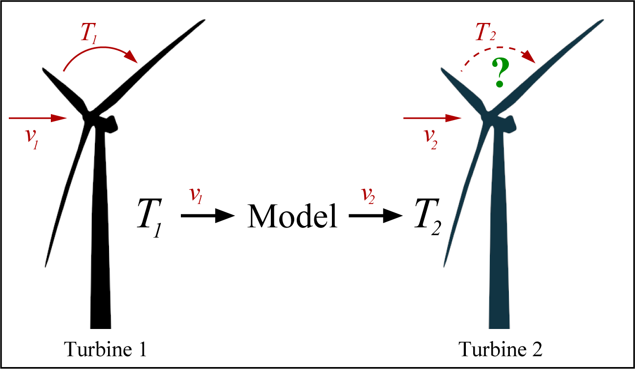
In this paper, we propose a recent model for reconstructing the increment statistics of the torque in single wind turbines as a tool for estimating fatigue loads, not only of that wind turbine, but also of its neighboring ones. As sketched in Figure 1, we use the wind speed and torque data series of one wind turbine (Turbine 1) to derive our stochastic model, which describes statistically the evolution of the torque subject to the observed wind speed. We assume that the response of similar wind turbines to the wind speed shall yield similar values of their properties, such as the power, the blade bending moments or the torque on the main shaft. Therefore, we apply the derived stochastic model to another wind turbine (Turbine 2), where only the wind speed is measured on the nacelle. The outcome yields a series of torque estimates used for a fatigue analysis, including Markov matrices, rain flow counting statistics and the load duration distribution, which are then compared with the fatigue analysis of the respective torque measurements. The overall result is that our stochastic model retrieves accurate estimates of fatigue loads in any wind turbine within the same wind farm.

We start in Section 2.1 by describing the data analyzed, and in Section 2.2, the method is described in further detail. Our results for extracting the stochastic model are described in Section 3.1, and the fatigue analysis and fatigue estimate are presented and discussed in Section 3.2. Section 4 concludes the paper.

2. Data and Methodology

2.1. Wind Speed and Torque at Alpha Ventus

We analyze the set of measurements of the wind speed and torque taken at two different wind turbines in Senvion in the Alpha Ventus wind farm, namely Turbines AV4 and AV5, during the full month of January 2013.

In principle, our analysis could also be done for other types of loads instead of the drive torque. However, in this article, we focus on the fatigue on the drive train, since some of its components are known to be prone to failure. In the future, we aim at extending our analysis to other turbine components.

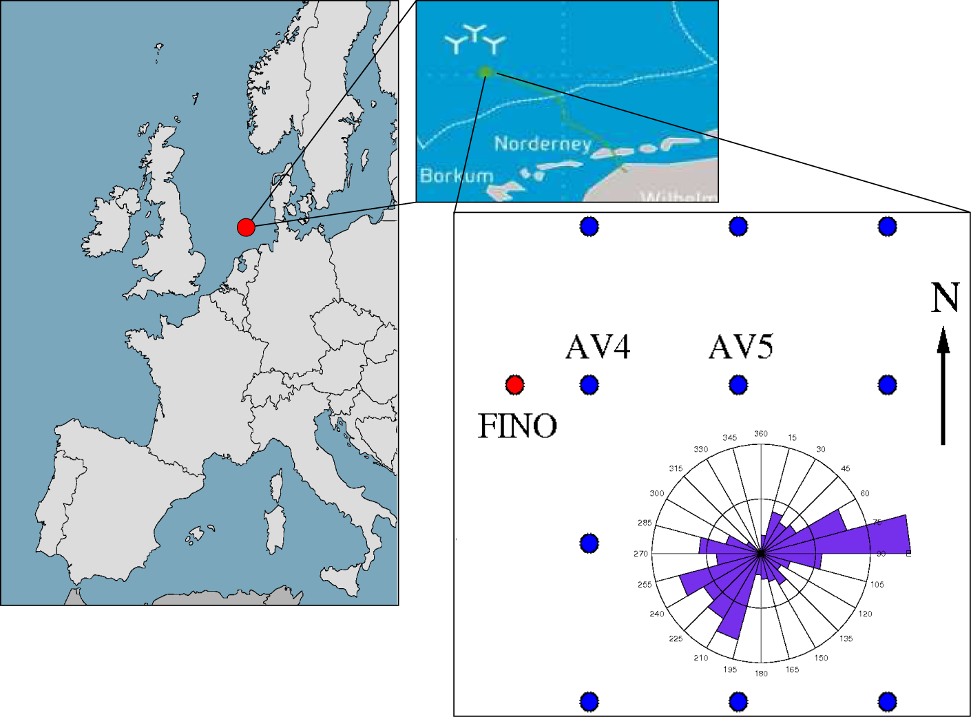
Figure 2 shows a sketch of the Alpha Ventus wind farm, the first off-shore wind farm in Germany, located at Borkum West in the North Sea, 54.3°N–6.5°W. As shown in the wind rose, during January 2013, the main wind direction lies between northeast and east.

The torque on the main shaft T is computed from the measurements of the power output P and the rotor rotational speed n, assuming neither mechanical nor electrical losses:

$$T=\frac{30}{\pi }\frac{P}{n}$$

(1)

with n in r.p.m., P in W and T in Nm. The sampling rate of the power output, rotational speed and, consequently, the torque is 50 Hz, and the sampling rate of the wind speed is 1 Hz. Since we need to use the same sampling rate for all data series, we only consider torque measurements each second, at instants for which a wind speed measurement also exists. In total, for Turbine AV4, we have 826,745 data points.

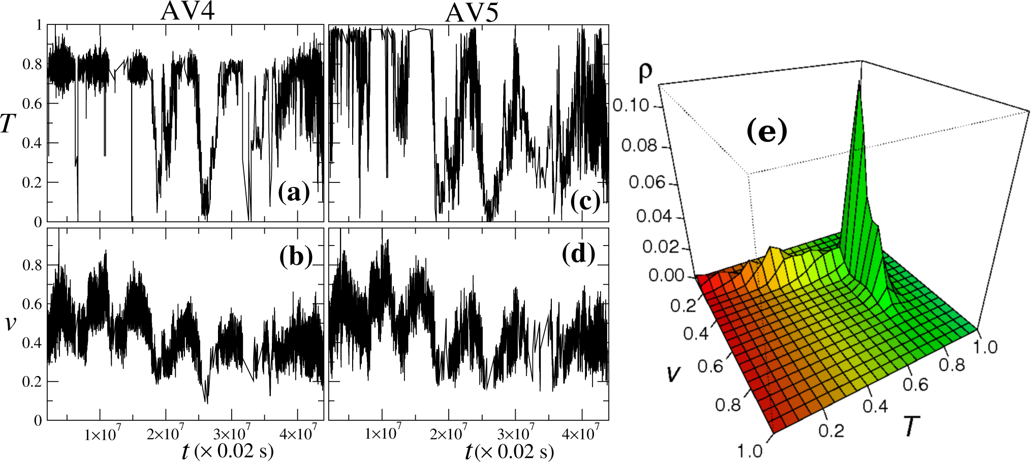
Both the wind speed and torque measurements are shown in Figure 3 and are according to the torque-speed curve known in the literature [4,8,9]. As one sees, the torque at both wind turbines, in Figure 3a,c, shows periods of high power production (large values), alternating with pronounced decreases and subsequent increase, during which large fluctuations occur. The largest values of the torque observed for Turbine AV4 (Figure 3a) are not so close to the maximum observed value as the values observed in the torque for AV5 (Figure 3c). As for the wind speed observed for both turbines (Figure 3b,d), this increases and decreases in an oscillating manner and simultaneously in both turbines, but showing no clear periodic pattern. In Figure 3e, one also plots the joint probability density function (PDF) for both the wind velocity and the torque, a plot that will be of importance when interpreting the stochastic model introduced below.

All data series were analyzed according to all confidential protocols and were properly masked through normalization by their highest value, being here published with Senvion’s permission. Scientific conclusions are not affected by such data protection requirements.

Together with most of the properties measured at wind turbines, wind speed and torque have typically fluctuations occurring at different time spans, defining the series of increments, whose statistics describe the intermittency observed in the wind energy production [10]. In the particular case of the torque, the succession of torque increments is related to the so-called random load cycles, which are of importance for estimating fatigue loads.

From the physical point of view, the fatigue load at one wind turbine is roughly the time integral of load increments, or of some proper positive and monotonic function of the increments. Therefore, we consider the increments ΔT_τ(t)=T(t+τ)−T(t), taken with a fixed time gap τ. As reported in [9], for up to one hour or more, the torque increment distributions are clearly non-Gaussian. In Section 2.2, we will describe a framework that yields an evolution equation for the torque constrained to the wind speed observed at the same turbine. With such a framework, we reconstruct not only the torque observed at that same wind turbine, but also the torque observed at neighboring wind turbines, which we assume to respond similarly to the wind speed.

2.2. The Conditional Langevin Model for Turbine Loads

The Langevin approach is a framework developed from the pioneer work by Peinke and Friedrich in 1997 [11], which consists of a direct method for extracting the evolution equation of a stochastic series of measurements. Several applications were proposed and developed, e.g., in turbulence modeling, in medical Electroencephalographic monitoring and in stock markets. See [12] for a review. In the context of wind energy, this framework has shown the ability to predict power curves of single wind turbines [10,13,14], as well as of equivalent power curves for entire wind farms [15] and, also, to properly reproduce the increment statistics of power and torque in single wind turbines [9,10].

One considers a set of measurements X(t) in time t of one particular property x evolving according to the so-called Langevin equation defined by:

$$\frac{dx}{dt}=D^{(1)}(x)+\sqrt{D^{(2)}(x)}{\mathrm{\Gamma }}_t,$$

(2)

where Γ_t is a Gaussian δ-correlated white noise, i.e., 〈Γ(t)〉=0 and 〈Γ(t)Γ(t′)〉=2δ_ijδ(t−t′).

The first term in the right hand-side incorporates the deterministic contributions in the process, yielding the drift function D⁽¹⁾, while the second terms models the diffusion, i.e., the total stochastic contributions accounting for the stochastic fluctuations, which are incorporated by function D⁽²⁾. The factor of 2 in the δ-correlation and the square root in the Langevin equation are usually chosen for convenience. Details can be found in [12].

Since the drift and diffusion function have a physical interpretation, one could apply the model in Equation (2) to a particular system and define ad hoc the functional shape of both functions from physical reasoning. In several cases, however, such an approach is not convenient; for instance, when considering properties that result from the interaction between a turbulent system, such as the atmosphere, and a complex technical device, such as the drive train in a wind turbine. In those cases, it is hard to derive drift and diffusion from first principles, and the one natural alternative to get information about their functional form is data analysis. In this work, we deal, therefore, with the inverse problem: having a set of measurements, is it possible to derive the drift and diffusion functions in order to reproduce the statistics of that set of measurements from the simple integration of Equation (2)?

The short answer is, yes, it is possible. The long answer has two main steps.

In the first step, one needs to test the data to ascertain if it can be taken as a Markovian series, i.e., if there is a time interval t_ℓ, the so-called Markov–Einstein length, for which, in the succession of measurements, the next value only depends on the present one and is independent of the values previous to it. In other words, one must test if:

$$\rho \left(X\left(t+t_{\ell }\right)|X(t),X\left(t-t_{\ell }\right),X\left(t-2t_{\ell }\right),\dots \right)=\rho \left(X\left(t+t_{\ell }\right)|X\left(t\right)\right)$$

(3)

holds, with ρ(x|y) representing the conditional probability density function (PDF) for observing x having observed y. This PDF can be extracted from the histograms of the dataset.

There are simple standard ways to perform this test [12], which typically compare three-point statistics, such as ρ(X(t+t_ℓ)|X(t),X(t−t_ℓ)) conditioned to a fixed value X(t−t_ℓ)=X^*, with the corresponding two-point statistics ρ(X(t+t_ℓ)|X(t)) and ascertaining which t_ℓ one obtains the best overlap, between both PDFs.

Though, when the measurements obey this Markov condition, the next step can be carried out, one advantage of this Langevin framework is that it also works in some cases where the Markov test fails. One such case is the presence of measurement noise [16,17], which opens a broad panoply of different practical situations where this framework is applicable. In the present case, though no measurement noise seems to be present, as reported below, the Markov condition is not perfectly fulfilled, as shown in Figure 4a. Still, it is important to stress here that it is possible to accurately estimate fatigue loads using such a framework.

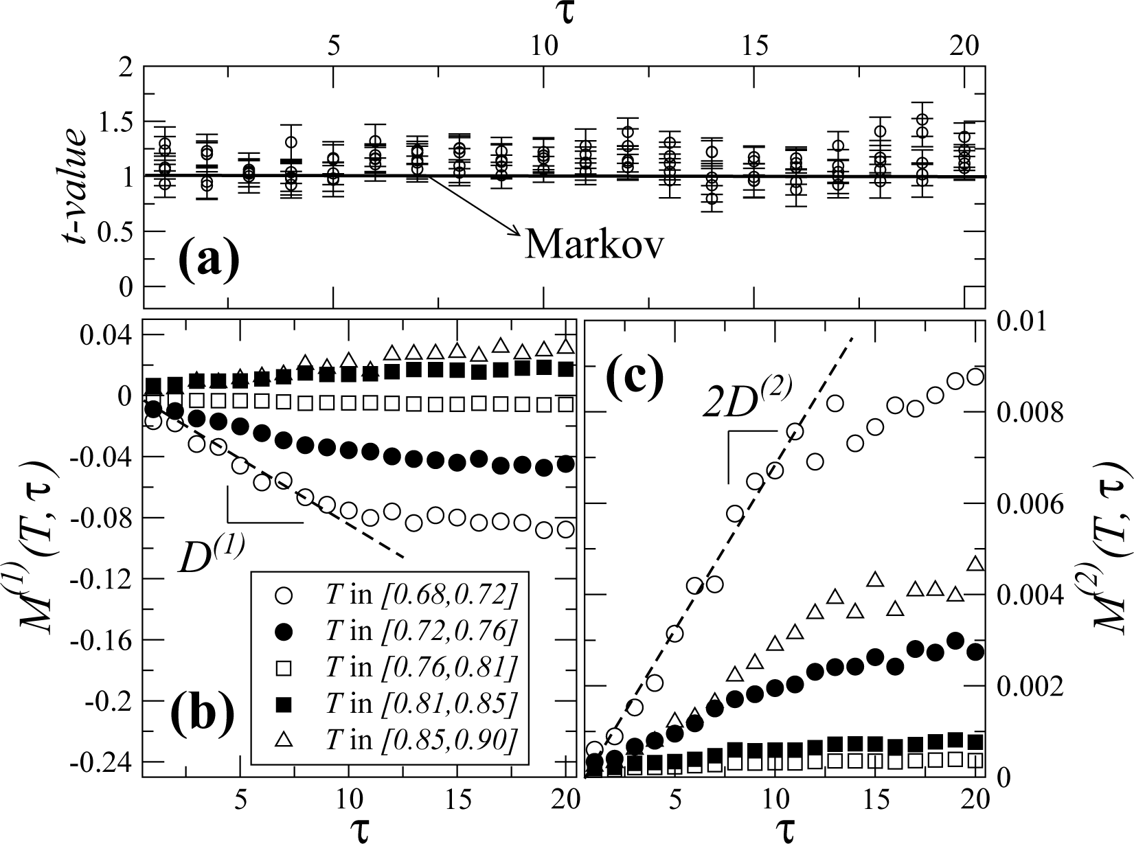
To test the Markov condition, we compute a t-value, as shown in Figure 4a. The Wilcoxon test is a statistical test used to test if Equation (3) holds. One assumes having two different series of values from independent random variables and tests whether the variables are identically distributed or not. The model retrieves a t-value, which when equal to the unit indicates perfect matching between both distributions in Equation (3). As we see from Figure 4a, though the observed t-values lie near the perfect fit value, they cannot always be taken as being one within numerical precision. While the Markov property is fulfilled only approximately, we show in this paper that load time series can be accurately reconstructed and fatigue loads accurately estimated.

For the second step, one needs to derive both functions, D⁽¹⁾ and D⁽²⁾, that fully define Equation (2). The derivation is performed through the computation of the corresponding first and second conditional moments [9], respectively:

$$M^{(1)}(x,\tau )=\langle X(t+\tau )-X(t)\rangle |{}_{X(t)=x}$$

(4a)

$$M^{(2)}(x,\tau )=\langle X(t+\tau )-X{(t)}^2\rangle |{}_{X(t)=x}$$

(4b)

where 〈 〉|_X(t)=x indicates the average over the full time series, whenever X(t) takes the value x.

Figure 4b,c shows the first and second conditional moments for five different values of the torque at AV4. Taking the slope of the linear regression for each conditional moment yields the corresponding coefficients D⁽¹⁾ and D⁽²⁾. Indeed, it can be shown [18] that drift and diffusion functions in Equation (2) are, apart from a multiplicative constant (1/k!), the derivative with respect to the time gap τ of the first and second conditional moments, respectively, which, for arbitrary order k, is defined as:

$$D^{(k)}(x)=\underset{\tau \to 0}{\lim }\frac{1}{k!}\frac{M^{(k)}\left(x,\tau \right)}{\tau }.$$

(5)

Therefore, drift (k = 1) and diffusion (k = 2) can be directly extracted from the datasets. For accuracy purposes, a correction is introduced for the diffusion function [19], where instead of the second condition moment M⁽²⁾(x, τ), one considers:

$$M_{cor}^{(2)}\left(x,\tau \right)=M^{(2)}\left(x,\tau \right)-{[M^{(1)}\left(x,\tau \right)]}^2.$$

(6)

Within a sufficiently low range of τ values, typically between five and ten time steps of the set of measurements, the conditional moments depend linearly on τ. Thus, for each value x, both D⁽¹⁾(x) and D⁽¹⁾(x) are given by the slope of the linear interpolation of the corresponding conditional moments.

It is worth mentioning that, as known in previous studies [16,17], the existence of an offset in the conditional moments indicates the presence of measurement noise in the data. As shown in Figure 4b,c, the linear interpolations cross the origin, and no offset seems to exist. Therefore, one can say that measurement noise is not significant in the datasets analyzed in this paper.

On top of these two steps, one important assumption must be added: the set of measurements must be stationary. This is of course not the case for torque series at one wind turbine. To overcome this shortcoming, it was recently proposed that [9,20] one should consider the succession of measurements of the torque corresponding to a sufficiently narrow range of speed values. Considering only this subset of torque values governed by what we named the conditioned Langevin equation [9], one observes that the statistical moments of the torque value distribution are approximately constant, depending only on the wind speed (not shown). The conditioned Langevin equation used here as the model is defined as:

$$\frac{dT}{dt}=D^{(1)}\left(T,v\right)+\sqrt{D^{(2)}\left(T,v\right)}{\mathrm{\Gamma }}_t,$$

(7)

where, for our purposes, T represents the torque at the wind turbine and v is the wind speed.

For such an extension of the Langevin approach, now conditioned to the values the wind velocity, all of the procedures described above are applied separately for the value of the wind velocity. This means that, having the full series of the torque at AV4, one now filters out all values, except those observed, together with a given wind velocity v = v^*, and computes, one for each, the conditional moments:

$$M_{v^{\ast }}^{{}^{(1)}}\left(T,\tau \right)=\langle T(t+\tau )-T(t)\rangle |{}_{T(t)=T,v(t)=v^{\ast }},$$

(8a)

$$M_{v^{\ast }}^{{}^{(2)}}\left(T,\tau \right)=\langle T(t+\tau )-T{(t)}^2\rangle |{}_{T(t)=T,v(t)=v^{\ast }}.$$

(8b)

Similarly, the Markov test was also performed for each wind velocity separately, as described above.

Having derived both drift and diffusion functions, a final test must be performed. Generically, one can compute from Equation (5) the coefficients D^(k)(x) of an arbitrary order k. However, according to Pawula’s theorem [18], in the case that D⁽⁴⁾ is zero or, for practical purposes, it is negligible in comparison with the drift and the diffusion, all coefficients of order k ≥ 3 are also negligible.

Figure 5a,b shows the drift and diffusion, respectively, as a function of both the torque and the wind velocity. The projection along the velocity is shown in Figure 5c,d, where one identifies a transition approximately at T = 0.75 (in units of T_max) where the drift depends linearly on the torque, while the diffusion depends quadratically on the torque. Here, only the range [0, 0.85] is plotted; as shown in Figure 3e, beyond this range, no significant statistics is observed. Both D⁽¹⁾ and D⁽²⁾ were computed for 21 bins in the torque, covering only the observed range of values at each particular velocity bin (21 bins). Since, for each velocity bin, this range of values is different and covers solely and partially the full range T ∈ [0,1], Figure 5c,d shows a number of T-values larger than 21.

From the plots, Figure 5a,b, one sees that the value T = 0.75 is first attained for wind velocities around v = 0.4 (in units of v_max). These two values also separate two different regions when observing the joint pdf (see Figure 3e). Above this value, the controller at a wind turbine starts operating. Below that velocity, the drift is almost absent, and diffusion decays with the magnitude of the velocity. Considering Equation (7), a closer look into the plots in Figure 5 enables one to physically interpret D⁽¹⁾ and D⁽²⁾ in a stochastic model for the torque conditioned to the wind velocity.

In general [18], the drift measures the force driving a specific property to increase or decrease in time, while the amplitude in the diffusion coefficient measures the amplitude of a fluctuation around that driven motion. Having such a physical interpretation in mind and looking again at the plots in Figure 5, one can conclude that the controller starts operating around v = 0.4. Indeed, for this value, the drift coefficient D⁽¹⁾ shows a linear dependence on the torque with a negative slope: when the torque increases, the controller acts in order to decrease it, and vice versa. Simultaneously, diffusion depends quadratically on T. Moreover, below the velocity threshold for controller operation, the drift almost vanishes with a diffusion that decreases with the magnitude of the wind velocity: no force is driving the torque for this range of wind velocities, and the magnitude of torque fluctuations increases with the wind velocity.

3. The Stochastic Model for Fatigue Loads

Using the Langevin framework described in the previous section, we next apply it to Wind Turbine AV4 in order to extract a stochastic model for the torque, which is assumed to hold for any Alpha Ventus turbine of the same model. Then, we use the set of wind speed measurements at a different wind turbine, namely AV5, for generating the increments of the torque at this second turbine and compare it with the torque measurements. Finally, we show that the estimate of the fatigue loads at Wind Turbine AV5 are statistically the same for the empirical torque measurements and for the reconstructed series.

3.1. Reconstruction of Non-Stationary Time Series

In a previous paper [9], we have shown that the anomalous wind statistics are responsible for the intermittent time evolution of the load in single wind turbines, promoting additional fatigue of the turbine itself. The approach used there follows from the method proposed in [3,10] for the power output of singl turbines.

We now use the model introduced in our previous work, with the drift and diffusion functions, D⁽¹⁾ and D⁽²⁾, in Figure 5, extracted according to the framework described above for Turbine AV4, and apply it to generate the torque in a neighboring wind turbine, namely AV5. For reconstructing the torque at AV5, one integrates the stochastic Equation (7) in time, using the usual schemes for the integration of stochastic equations [12,18]. Concerning one important aspect, if the number of simulations is an advantage for our work, we have simulated our results several times independently and obtained no new insights. When integrating our model, it is the running time, i.e., the time span over which we simulate, that increases the statistics and consequently the precision of the reconstructed increment statistics.

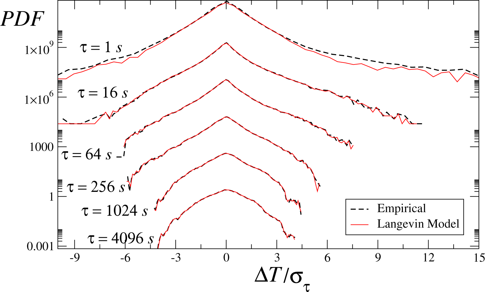
The wind speed measurements taken at AV5 are used as input data and initialize the differential evolution equation, Equation (7), with the first measurement of the torque at this same wind turbine. The reconstruction of the increment statistics is plotted in Figure 6, with solid lines, together with the empirical distributions in dashed lines. While for low values of the time span τ, the extreme fluctuations are not completely well reproduced, above a time window larger than a few seconds, the fit between the measurements and the model is very good.

In the inset of Figure 5b, one sees that the typical values of D⁽⁴⁾ are of the order of 1% to 2% of the D⁽²⁾ values. As explained above, such low values corroborate the applicability of the method to these datasets.

For practical purposes, one should briefly stress that the model described here is suitable for cases where the sampling frequency of the wind speed and torque data are high enough. A sparse sampling of the wind speeds leads to a poor increment statistic and, consequently, is not accurate enough for estimating fatigue loads.

Having a proper way for reconstructing the increment statistics, one is now in a position to use the reconstructed series of loads for estimating the fatigue at AV5 and compare it with the empirical fatigue analysis.

3.2. Fatigue Analysis and Estimate

To test the capability of the Langevin framework to predict fatigue loads in a wind farm, we next present a comparative fatigue analysis between both the empirical datasets at AV4 and AV5 and the reconstructed dataset for AV5 only. This comparative analysis is based on three standard tools, namely Markov matrices of the number of cycles, the rain flow counting procedure and the load duration distribution. All of these tools are based on the concept of load cycle, which is the observed load fluctuation between two successive local minima or maxima of the load.

The rain flow counting method was proposed in the late nineteen sixties by Endo and Matsuishi [21] and became the most standard algorithm for cycle-counting during the last few decades, due to its ability for accurately predicting the fatigue loads in a sequence of non-constant cycles. It has been defined in a mathematically rigorous way by Rychlik in [22].

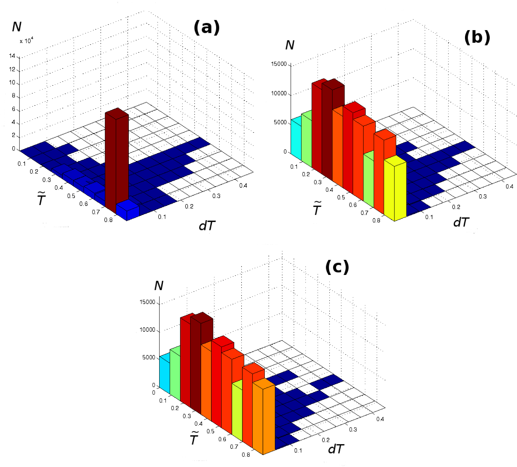
In the context of fatigue analysis, the so-called Markov matrix retrieves the number of load cycles of a given amplitude ΔT as a function of the mean value of the observed load during each load cycle $\tilde{T}$. The term “Markov matrix” is used here for the plots shown in Figure 7 and is standard in the context of engineering for fatigue analysis. It should not be confused with the terms “Markov process” and “Markov condition”, used in previous sections, standard in the field of statistical physics, with which other different matrices, e.g., transition matrices, may be associated. In Figure 7a,b, we plot the Markov matrix of the observed load for AV4 and AV5, respectively. In both cases, most of the cycles have an amplitude smaller than 0.5, in units of the maximum value of the load. While at AV4, such amplitudes are observed for large loads, around 0.7, at AV5, such amplitudes are also observed in the remaining range of values, being predominant in the lower load region, around 0.3. The reconstructed load series for AV5, shown in Figure 7c, however, retrieves a good estimate of the full range of values, still with the same deviation for the highest load values.

The difference between the observed Markov matrices for AV4 and AV5, with AV5 showing a broader range of torque strengths, can be explained by considering the location of each turbine with respect to the main wind directions. As sketched in Figure 2, AV4 lies westerly from AV5, which lies in the middle of four neighboring wind turbines. Further, the main wind directions are southwest and east-northeast. Thus, the wake effects on AV5 should be stronger than on AV4, and consequently, the optimal operation is not as frequent.

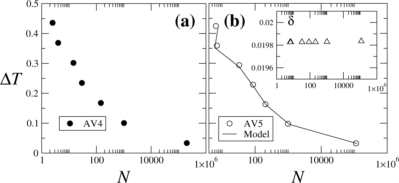
Similarly to what we did with Markov matrices, we compute the rain flow counting (RFC) for AV4 (bullets in Figure 8a) and AV5 (circles in Figure 8b). While the RFC spectra of AV4 and AV5 are qualitatively different, the Langevin model applied to AV5 retrieves a correct estimation of the rain flow spectra. In the inset of Figure 8b, one sees the relative error:

$$\eta =\frac{A_r-A_e}{A_r},$$

(9)

where A_r and A_e are the amplitudes observed for the real and estimated values. The relative error of the rain flow counting for the estimates is less than 2%.

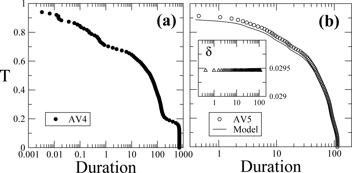
Finally, the load duration distribution (LDD) shows the amount of time a load with a given amplitude is observed, retrieving the energy consumed by the system, which is no more than the integral of the load duration distribution. As shown in Figure 9, similarly to what is observed for the RFC, the LDD is also properly reproduced for sufficiently sampled loads (the largest values).

Our approach is not based on a specific wake model. From our analysis, we see that the measured wind speed at the hub seems to contain sufficient information about the wake, so that the loads, including the extra load due to the wake, can be grasped by our approach.

4. Conclusions

In this paper, we applied a framework to one single turbine of the Alpha Ventus wind farm for reproducing the loads observed in other similar wind turbines of the same wind farm. The framework consists of the derivation of a stochastic evolution equation for the loads constrained to the wind speed observed at each wind turbine. Using rain flow counting methods and load duration distributions for empirical and modeled data, we show that our framework is able to accurately estimate fatigue loads. In a more general context, this procedure can be applied to other properties one wants to access for monitoring and controlling wind turbines.

We stress that the coefficients used to reconstruct the torque at the second turbine are obtained only from the torque and wind velocity at the first turbine. The torque reconstruction is then performed by taking the wind velocity at the second turbine as the input parameter. Notice that the coefficients are taken directly from the numerical derivation (Figure 5) in only one realization. This is possible due to the coupling between v and T, which is assumed to be the same for both turbines.

Two points should be stressed for future work. First, the conditional Langevin model here presented and applied has some limitations. Since it is based on the integration of a stochastic differential equation of the load, using empirical input (the wind velocity) in time periods during which no measurements are available, additional assumptions would have to be made for reconstructing the torque during that period. Moreover, our analysis assumes that the wind velocity field to which the turbine reacts can be completely described by the single anemometer measurements; though such an assumption can be taken as a first approximation to the wind velocity field, some properly-defined, rotor-effective velocity may improve the reconstruction in our model.

Second, having shown the ability of our method to predict one particular load type, namely the one on the drive train, a systematic study of how it works for the rest of the loads on a wind turbine shall proceed. These points will be addressed in future work.

References

- Johnson, G.L. Wind Energy Systems; Kansas State University: Manhattan, KS, USA, 2006. [Google Scholar]
- Mücke, T.; Kleinhans, D.; Peinke, J. Atmospheric turbulence and its influence on the alternating loads on wind turbines. Wind Energy 2011, 14, 301–316. [Google Scholar]
- Milan, P.; Wächter, M.; Peinke, J. Turbulent Character of Wind Energy. Phys. Rev. Lett. 2013, 110. [Google Scholar] [CrossRef]
- Burton, T.; Sharpe, D.; Jenkins, N.; Bossanyi, E. Wind Energy Handbook; Wiley: Hoboken, NJ, USA, 2001. [Google Scholar]
- Moriarty, P. Database for validation of design load extrapolation techniques. Wind Energy 2008, 11, 559–576. [Google Scholar]
- Freundenreich, K.; Argyriadis, K. Wind turbine load level based on extrapolation and simplified methods. Wind Energy 2008, 11, 589–600. [Google Scholar]
- Ragan, P.; Manuel, L. Comparing Estimates of Wind Turbine Fatigue Loads using Time-Domain and spectral Methods. Wind Eng 2007, 31, 83–99. [Google Scholar]
- Rinn, P.; Wächter, M.; Peinke, J. Carl von Ossietzky University of Oldenburg, Oldenburg, Germany, Private communication. 2014.
- Lind, P.G.; Wächter, M.; Peinke, J. Reconstructing the intermittent dynamics of the torque in wind turbines. ArXiv E-Prints 2014, arXiv, 1404.2063. [Google Scholar]
- Mücke, T.A.; Wächter, M.; Milan, P.; Peinke, J. Langevin power curve analysis for numerical wind energy converter models with new insights on high frequency power performance. Wind Energy. [CrossRef]
- Friedrich, R.; Peinke, J. Description of a turbulent cascade by a Fokker-Planck equation. Phys. Rev. Lett. 1997, 78. [Google Scholar] [CrossRef]
- Friedrich, R.; Peinke, J.; Sahimi, M.; Tabar, M. Approaching complexity by stochastic methods: From biological systems to turbulence. Phys. Rep. 2011, 506, 87–162. [Google Scholar]
- Anahua, E.; Barth, S.; Peinke, J. Markovian Power Curves for Wind Turbines. Wind Energy 2008, 11, 219–232. [Google Scholar]
- Raischel, F.; Scholz, T.; Lopes, V.V.; Lind, P.G. Uncovering wind turbine properties through two-dimensional stochastic modeling of wind dynamics. Phys. Rev. E. 2013, 88. [Google Scholar] [CrossRef]
- Milan, P.; Wächter, M.; Peinke, J. Stochastic modeling and performance monitoring of wind farm power production. J. Renew. Sustain. Energy. 2014, 6. [Google Scholar] [CrossRef]
- Boettcher, F.; Peinke, J.; Kleinhans, D.; Friedrich, R.; Lind, P.G.; Haase, M. Reconstruction of complex dynamical systems affected by strong measurement noise. Phys. Rev. Lett. 2006, 97. [Google Scholar] [CrossRef]
- Lind, P.G.; Haase, M.; Boettcher, F.; Peinke, J.; Kleinhans, D.; Friedrich, R. Extracting strong measurement noise from stochastic time series: Applications to empirical data. Phys. Rev. E. 2010, 81. [Google Scholar] [CrossRef]
- Risken, H. The Fokker-Planck Equation; Springer: Berlin, Germany, 1984. [Google Scholar]
- Gottschall, J.; Peinke, J. On the definition and handling of different drift and diffusion estimates. New J. Phys. 2008, 10. [Google Scholar] [CrossRef]
- Milan, P.; Wächter, M.; Peinke, J. Wind Energy: A Turbulent, Intermittent Resource; Private Communication; Springer: Berlin, Germany, 2013. [Google Scholar]
- Matsuishi, M.; Endo, T. Fatigue of Metals Subjected to Varying Stress; Japan Society of Mechanical Engineers: Fukuoka, Japan, 1968; pp. 37–40. [Google Scholar]
- Rychlik, I. A new definition of the rainflow cycle counting method. Int. J. Fatigue. 1987, 9, 119–121. [Google Scholar]
© 2014 by the authors; licensee MDPI, Basel, Switzerland This article is an open access article distributed under the terms and conditions of the Creative Commons Attribution license (http://creativecommons.org/licenses/by/4.0/).
Share and Cite
Lind, P.G.; Herráez, I.; Wächter, M.; Peinke, J. Fatigue Load Estimation through a Simple Stochastic Model. Energies 2014, 7, 8279-8293. https://doi.org/10.3390/en7128279
Lind PG, Herráez I, Wächter M, Peinke J. Fatigue Load Estimation through a Simple Stochastic Model. Energies. 2014; 7(12):8279-8293. https://doi.org/10.3390/en7128279
Chicago/Turabian StyleLind, Pedro G., Iván Herráez, Matthias Wächter, and Joachim Peinke. 2014. "Fatigue Load Estimation through a Simple Stochastic Model" Energies 7, no. 12: 8279-8293. https://doi.org/10.3390/en7128279