Anticipating and Coordinating Voltage Control for Interconnected Power Systems


Abstract
: This paper deals with the application of an anticipating and coordinating feedback control scheme in order to mitigate the long-term voltage instability of multi-area power systems. Each local area is uniquely controlled by a control agent (CA) selecting control values based on model predictive control (MPC) and is possibly operated by an independent transmission system operator (TSO). Each MPC-based CA only knows a detailed local hybrid system model of its own area, employing reduced-order quasi steady-state (QSS) hybrid models of its neighboring areas and even simpler PV models for remote areas, to anticipate (and then optimize) the future behavior of its own area. Moreover, the neighboring CAs agree on communicating their planned future control input sequence in order to coordinate their own control actions. The feasibility of the proposed method for real-time applications is explained, and some practical implementation issues are also discussed. The performance of the method, using time-domain simulation of the Nordic32 test system, is compared with the uncoordinated decentralized MPC (no information exchange among CAs), demonstrating the improved behavior achieved by combining anticipation and coordination. The robustness of the control scheme against modeling uncertainties is also illustrated.1. Introduction
The introduction of the competitive market into the electricity industry, due to the deregulation and liberalization of electrical power systems, has created economic incentives for power systems to operate closer and closer to their safety and stability limits [1]. This, together with the larger and less predictable power flows, due to the increased use of renewable energy resources, leads to the formation of multi-area power systems. Each area is controlled by its corresponding control agent (CA) operated by an independent transmission system operator (TSO) [2]. Note that although CAs are not necessarily the same as TSOs and several CAs may be operated by a single TSO, throughout this article, we use TSO and CA as interchangeable terms.
The areas are typically interconnected through power transmission corridors that may carry heavy power flows in order to economically establish a common open electricity market and, technically, hopefully, to ensure a greater security margin, through the sharing of active/reactive power reserves. This interconnectedness, on the other hand, makes the large-scale power systems even more complex and harder to control by increasing the probability of creating more complicated loops that may destabilize the system, making it more vulnerable to global collapse, initiated by a local fault [3]. In this paper, we will deal with a given power system, and the decomposition will be based on the electrical distance of buses from each other.
Voltage collapse, as a calamitous result of unmitigated local voltage instability, can often lead to a blackout in the system [2]. In the context of large-scale multi-area power systems, it happens frequently that a local initiating disturbance in one area triggers some local control actions in its own area, which, in turn, triggers further disturbances in the neighboring areas, causing some undesirable control actions by their neighbors, and eventually, a cascade of possibly wrong control actions leads the overall system to a final collapse. An example is the notable incident that Europe's interconnected power grid experienced in November, 2006. The final report released by UCTE, recently renamed ENTSO-E, the coordinator of 41 TSOs in 34 European countries, identifies three main causes for this incident. One of these main causes was poor inter-TSO coordination, as the other European TSOs did not receive information on the control actions taken by German TSO E.ONNetz [4].
Our earlier work [5] proposes an effective anticipation and coordination paradigm, a so-called distributed communication-based model predictive control (DCMPC) approach, for properly coordinating the local control actions of load tap changing transformers [load tap changing transformers (LTCs)] taken by many communicating CAs, in order to maintain multi-area power system voltages within acceptable bounds in the time scale of typically one second to several minutes. This work clearly complements our previous work [5] by way of considering several issues that were deemed to be necessary to tackle in the current article. The main contribution of this paper is highlighted below:
The DCMPC scheme enjoys the joint contribution of anticipation and coordination. In order to identify the sole contribution of coordination in the improved performance of the DCMPC and to justify that the added complexity (by requiring communication between areas) is indeed needed to stabilize the system, the DCMPC-based results are compared with an uncoordinated decentralized MPC approach;
The robustness of the DCMPC against modeling uncertainties is assessed. This is very important, as the DCMPC is a model-based scheme;
The DCMPC scheme complements (and does not replace) the existing secondary control layer of a generic voltage control hierarchy. Thus, the feasibility of practical implementation of the DCMPC in the current existing voltage control schemes is also briefly discussed.
The remainder of this paper is organized as follows. The need for anticipation and coordination of local control actions in multi-area power systems for an effective voltage control is illustrated in Section 2. A further elaboration of the DCMPC scheme is given in Section 3. Next, Section 4 presents simulation results with the uncoordinated decentralized MPC obtained from time-domain simulation of the realistic well-known Nordic32 test system. The robustness of the DCMPC is illustrated in Section 5. The practical implementation issues are discussed in Section 6. Possible extensions of the DCMPC are described in Section 7. Finally, conclusions are drawn in Section 8.
2. The Need for Anticipation and Coordination
The anticipation and (more importantly) coordination of the effect of control actions in a network of many interacting components, in which each component is controlled by an independent CA, is a very challenging problem. The nonlinearity, especially arising from saturation, makes this even more important. Indeed, anticipation and coordination seems to be necessary in any network of interacting components in which a local perturbation can lead to global performance degradation. Some examples are:
voltage control in multi-area power systems;
control of traffic lights in an urban traffic network;
on-ramp metering to control freeway traffic, taking overflow into neighboring roads into account;
flood/irrigation control, where controllable gates can regulate the flow of water.
The DCMPC approach in this article is applied, as a case study, to the voltage control problem of electrical power systems. However, the DCMPC is generally applicable to many large networks of interacting dynamic components. It is useful whenever both anticipation (implemented via the model-based prediction of the effects of a local control action over a sufficiently long window of time) and coordination (avoiding the overall system being destabilized by unintended interactions between local control actions) are needed.
2.1. The Need for Anticipation
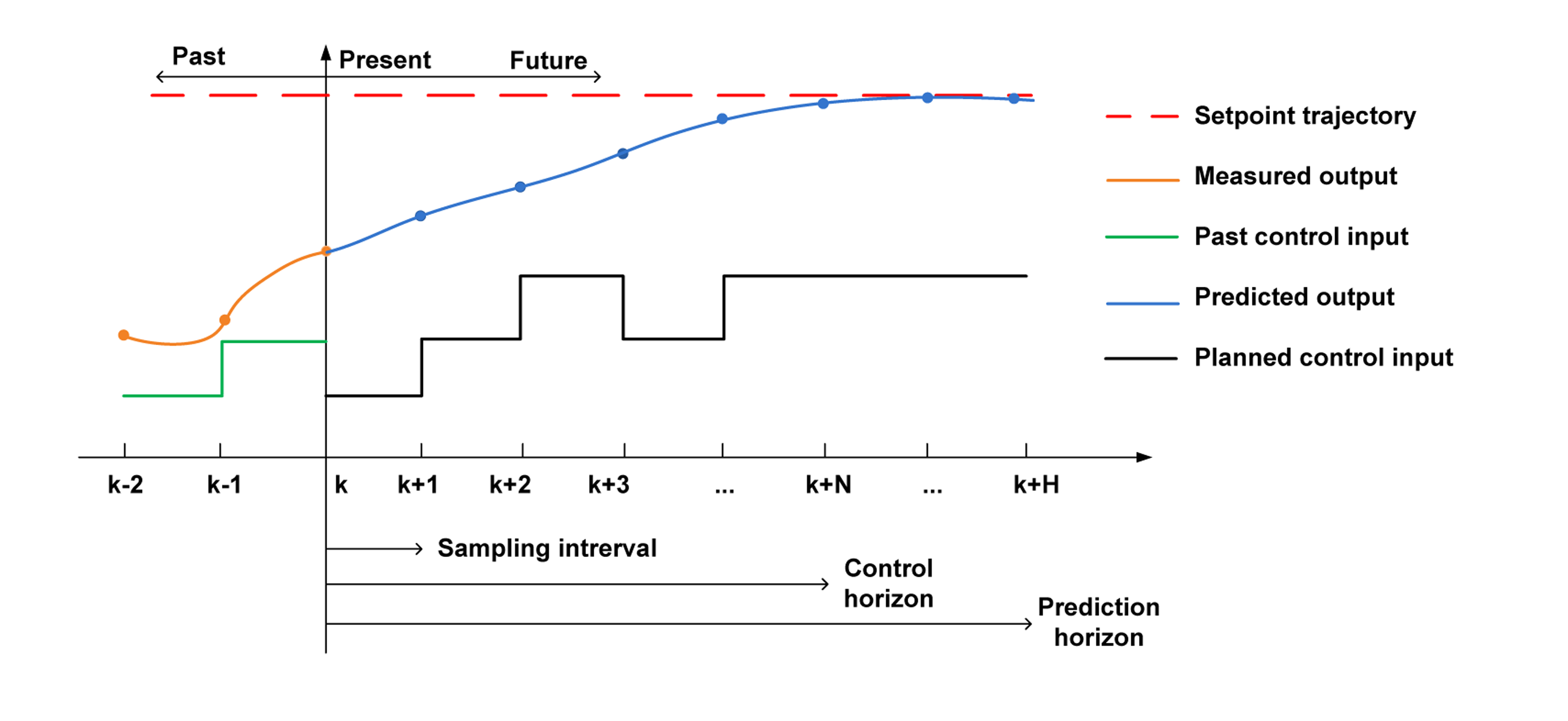
One of the most successful classes of closed-loop model-based anticipating schemes is the model predictive control (MPC) paradigm, also called receding/moving horizon control. MPC relies on an estimate of the current system states at discrete time instant tk = k × Tc and an explicit model of the system in order to predict the future output behavior via simulation over a finite window [tk,…, tk+H], for a set,
 , of allowable control sequences u = {u(tk), u(tk+1),…, u(tk+N−1)}, where u ∈
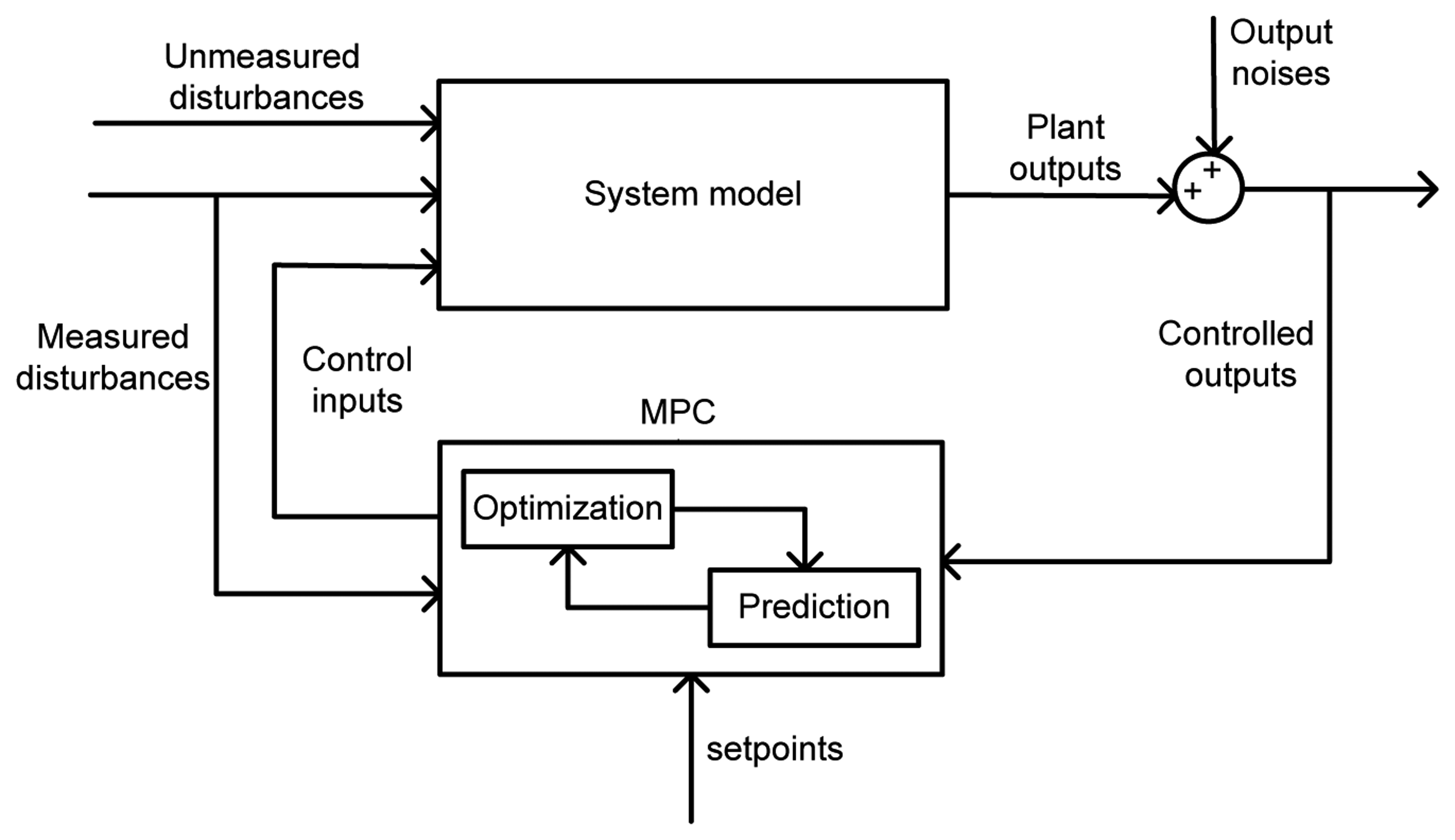
, 0 < N ≤ H, calculating the corresponding performance criterion. Then, only the first element, u*(tk), of the selected best sequence, u*, at time tk is implemented at the present time instant, tk. All these calculations are repeated, using new observations at the next time instant, tk+1, each time predicting performance over a shifted window with the size of H × Tc [5]. A schematic representation of MPC is shown in Figure 1. Figure 2 shows the inherent feedback nature of the MPC and illustrates that in order to find the k–th control action, u(tk), MPC operates in successive estimation and optimization steps.
, of allowable control sequences u = {u(tk), u(tk+1),…, u(tk+N−1)}, where u ∈
, 0 < N ≤ H, calculating the corresponding performance criterion. Then, only the first element, u*(tk), of the selected best sequence, u*, at time tk is implemented at the present time instant, tk. All these calculations are repeated, using new observations at the next time instant, tk+1, each time predicting performance over a shifted window with the size of H × Tc [5]. A schematic representation of MPC is shown in Figure 1. Figure 2 shows the inherent feedback nature of the MPC and illustrates that in order to find the k–th control action, u(tk), MPC operates in successive estimation and optimization steps.
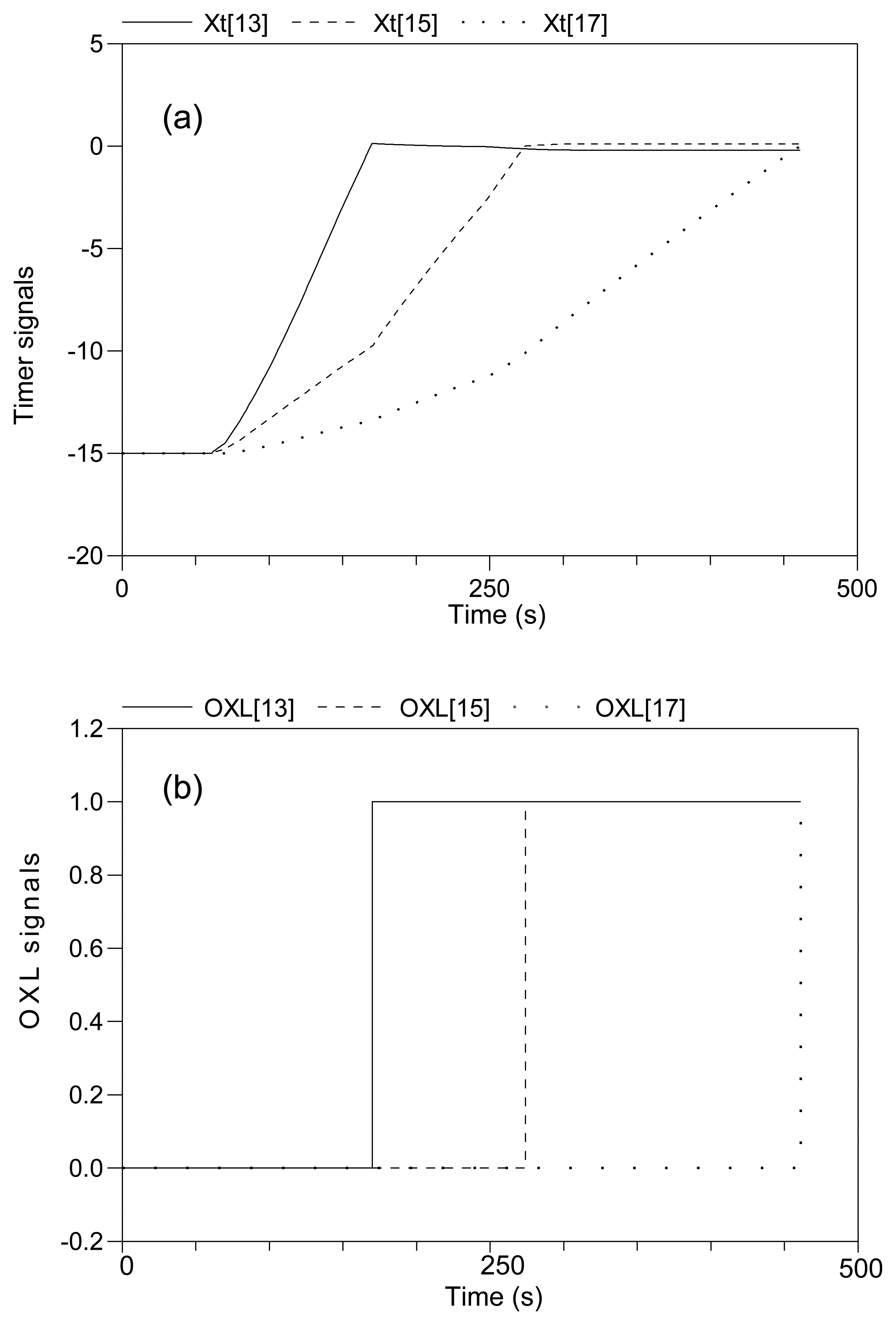
Anticipation/prediction is a very useful means for designing an on-line, well-performing, long-term voltage controller. The anticipating voltage controller can anticipate, within a prediction window [tk, …, tk+H), for example, the activation of over excitation limiter of synchronous generators [over excitation limiters (OXLs)], moving towards reaching the maximum physical tap limits for LTCs, and deviating too much from the prescribed voltage bounds for buses. The controller will then effectively use this anticipation, to compare several possible actions in order to select the optimal control sequence that, whenever possible, does not violate any of the operational and security constraints.
The model-based simulations for the local anticipating controllers must be fast enough in order to be applicable for real-time applications, such as on-line voltage control. We have developed, in [6], a sufficiently fast simulator, based on a hybrid system model paradigm to formulate the long-term voltage control problem in an MPC framework. The requirement of MPC-based schemes that a dynamical model must be known is certainly a limitation, especially for electrical power systems, where the local loads are not known accurately and where frequent changes of the generation and transmission resources can be expected. However, the inherent feedback of an MPC provides enough robustness against modeling errors. Moreover, the DCMPC design requires, for each local CA, a reduced-order dynamic model of the immediate neighbors only, and not of the distant areas.
2.2. The Need for Coordination
The case study of voltage control in large-scale multi-area power systems is an interesting application for coordinated control, as the poorly coordinated (or uncoordinated) operation of the areas may increase the risk of blackouts. In other words, in highly-coupled multi-area power systems, the creation of destabilizing loops as a reaction to a local disturbance, due to the complicated interaction among CAs, can eventually lead to a voltage collapse. Thus, the control actions taken by (at least) neighboring CAs must be coordinated. It is noteworthy that the voltage in electrical power systems is, by nature, a “local” variable, unlike frequency, which is a “global” variable. This means that, in multi-area power systems, only electrically close areas interact for voltage control, and thus, there is no need to involve distant areas with negligible common interest in solving a local optimization problem. The latter makes possible a decomposition approach for voltage control, where the voltage control still remains a prerogative of the local utilities.
In the case of a simple and small interconnected power system, e.g., power systems consisting of, at most, two areas, or in the conventional radial distribution networks with the integration of distributed generation units, the voltage coordination may be obtained by heuristic ad hoc schemes based on off-line assessment of utilities [7,8]. As the size and heterogeneity of the network increases or in the case of a complex meshed structure, coordination can become a very challenging or even infeasible problem.
Designing a possible coordination strategy is a major challenge involving many issues, such as what information to communicate, how to avoid the need that each area knows the global model and, last, but not least, the choice of abstraction level of the models.
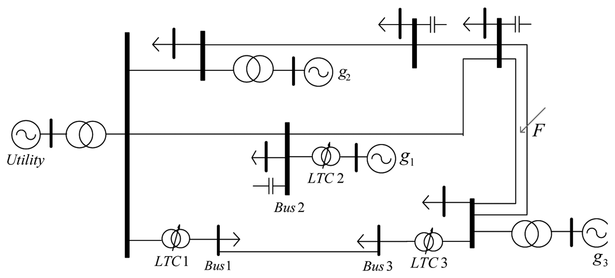
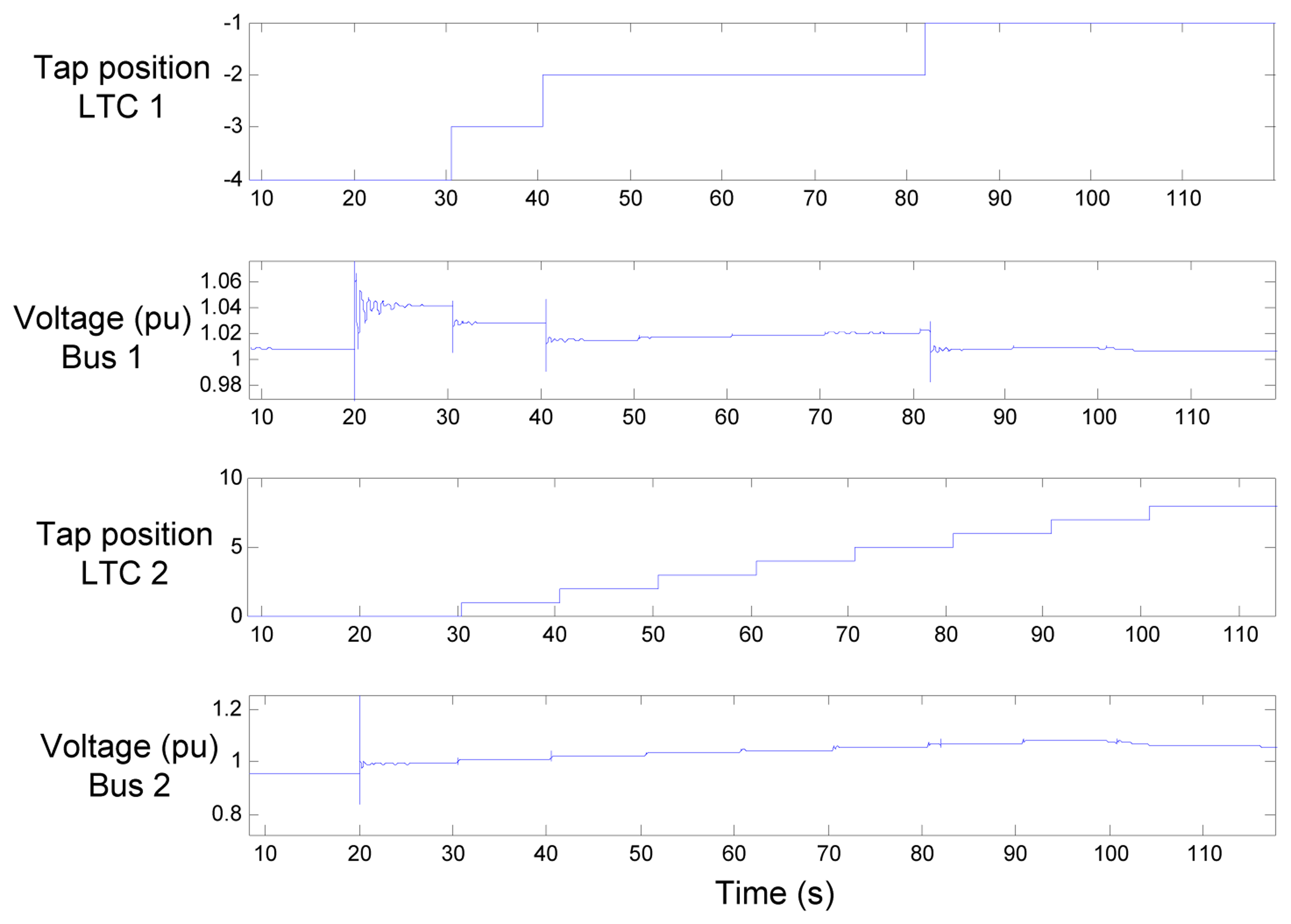
The following example of the 12-bus meshed test system, shown in Figure 3, is adopted from [9] to illustrate why coordination is necessary for voltage control in power systems and how different local control actions can trigger each other. The three identified local control agents CAi, i = 1, 2, 3 try to use LTCs 1, 2 and 3 to locally maintain the voltage of Buses 1, 2 and 3 within an upper and a lower bound [0.98, 1.02] p.u. by using a standard deadband strategy. Two pairs of “LTC moves-bus voltage”, namely (LTC 1, Bus 1) and (LTC 2, Bus 2), are shown in Figure 4, following the outage of one of the parallel lines in the location, F, at t = 20 s. Following the fault, both LTCs, after a delay of 10 s, try to restore the corresponding local voltages. As one can see, the voltage of Bus 1 is already within its safety limit around t = 40 s, but still, one extra move around t = 82 s is observed. The reason is that LTC 2 causes the voltage at Bus 1 to drop below its threshold, again causing LTC 1 to activate its local deadband strategy. Thus, this extra move is indeed attributed to the interaction between LTC 2 and Bus 1 (via LTC 3 and Bus 3). A possible coordination scheme should aim, at least, at avoiding these kinds of interactions among local controllers (if more is not necessary).
3. Highlights of the DCMPC
The general characteristics of the DCMPC have been previously reported in [5,10]. The DCMPC is an effective anticipation and coordination paradigm for properly anticipating and coordinating the tap position changes of the local LTCs located in neighboring areas. The future behavior of the areas are effectively anticipated by assigning a local MPC to each area, and an additional active communication architecture on the planned control actions among neighboring CAs is established in order to avoid instability in the overall system. We employ (besides the detailed local model of each area) the reduced-order quasi steady-state (QSS) models [7] for the immediate neighboring areas. This is a reasonable assumption, since we deal in this paper with the long-term voltage instability—a relatively slow phenomenon ranging from several seconds to a few minutes—and thus, only the long-term dynamics are of primary interest. The well-known QSS approximation assumes that short-term, fast dynamics are infinitely fast and can be represented by their algebraic equilibrium equations instead of by their full dynamics. QSS simulation allows the obtaining of very much faster-than-real-time simulators for reasonably sized networks [7,10].
However, a simple PV approximation [11] is used to represent the distant areas as buses with constant voltage magnitudes and constant active power consumptions over the prediction horizon, H. Note that the reduced-order models for the immediate neighboring areas and the PV models for the distant areas are assumed to be given in the simulations, as we do not deal in this article with their identification/estimation. The local optimizations are done through exhaustive enumeration of all possible LTC future tap sequences (over a finite control horizon, N) and calculating the corresponding costs to identify the optimal LTC sequence at each discrete time tk. Thus, there is no iteration involved in the sense of reaching an optimal value. In this paper, we assume N = 3. ui ∈
i denote a candidate control sequence of LTC tap position changes and
i = {0, +1, −1}N × {0}H−N+1 the corresponding finite set of all admissible control sequences, the size of
i will be |
i| = 3N = 27. Note that 0, +1 and −1 refer resp.to having no tap movement, an upward tap movement and a downward tap movement, and no tap movement is considered in the interval [tk+N,…, tk+H].
The set of possible sequences of control values grows exponentially with the size of the network. Dealing with a very large-scale multi-area power system, such as the European interconnected network, some heuristics based on physical intuition would be needed in order to reduce the number of possible input sequences to be considered as possible MPC control, thus eliminating those that the designer knows in advance will almost certainly not be optimal. This paper serves as a proof-of-concept, and illustrates that for reasonably sized networks, as considered in this paper, the DCMPC is feasible for being applied in real time.
3.1. Decomposition Criterion
We decompose the overall power system into M interacting areas Ai, i ∈
 = {1,…, M}, each controlled by a local control agent CAi, i ∈
 = {1,…, M}. This decomposition, from a power system point of view, may be realized in several ways. In the most common practice, also adopted here, depending on the geographical structure of the system, a set of buses located at a relatively short electrical distance from each other are considered as one particular area. The advantage is that, because the electrical distances are proportional to the physical lengths of the interconnecting transmission lines, the voltage control areas (zones), as a result, are identified in advance and are assumed to remain unchanged during the real-time dynamic operation of the system. In other words, the areas are not affected by, for example, loading/generation conditions and/or faults and need not be re-identified after possible changes in the system operating conditions. However, areas may also be adequately determined by sensitivity analysis of the overall system with respect to the influence of the available controls. In this case, the boundaries of areas change dynamically during real-time system operation, and areas must be redefined periodically in order to better reflect the system topology and dynamic changes in the operating conditions [12].
This decomposition creates a very important “scalability” feature for the DCMPC scheme, which makes it suitable for dealing with large-scale multi-area power systems containing many distinct voltage control areas. This is thanks to the fact that each CA, in order to perform the local optimization, requires (in addition to the detailed local model) the QSS reduced-order models only of its few immediate neighboring areas (as well as limited information exchange only with them) and replaces the remaining distant areas by much simpler PV models without any information exchange. Thus, no matter how large the power system is, the computational complexity of the local calculations at each CA remains the same. Note that the decomposition criterion described above is applied to a given/existing power system with components already being physically in place, and the design of the system in order to best allocate the LTCs is out of the scope of this paper.
3.2. Hybrid System Models
In order to develop a sufficiently fast simulator to cope with the hybrid dynamic nature of the power systems' behavior, we adopted a hybrid system model to formulate the long-term voltage control problem to be controlled by MPC-based controllers [6]. A power system is advantageously considered as a composition (or network) of interacting hybrid dynamical system components. The formal hybrid automaton (HA) modeling paradigm is then employed to model the underlying mixed continuous and discrete-event dynamics of the physical components. More specifically, every individual component is represented by an HA (or parallel composition of several HAs), where the piecewise continuous dynamics are expressed by differential-algebraic equations (DAEs) and discrete events are represented by the set of events, E, of that HA, using Modelica® [13]. Note that the discrete-event dynamics are typically induced by local discrete control logics, such as LTCs, switched capacitor banks (CBs) and disturbances and/or by thresholds reached when some devices saturate, e.g., OXLs of synchronous generators.
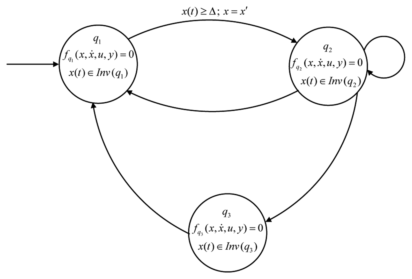
An HA is a dynamical system describing the time evolution of a system involving the interaction of both continuous and discrete state variables. For example, the HA of Figure 5 operates as follows, defining the possible evolutions for its hybrid states, (q, x) ∈ (Q, X). It starts in the initial state, (q1, x0) ∈ Init, where the corresponding dynamics represented by the DAE fq1 (x, ẋ, u, y; x(0) = x0) = 0 is followed, as long as x ∈ Inv(q1). As soon as the guard condition, Δ ∈ G(q1, q2), is fulfilled, the event e = (q1, q2) ∈ E occurs. This resets x to x′ ∈ R(e, x, ẋ, u, y), making a transition to state (q2, x) where the corresponding dynamics fq2 (x, ẋ, u, y) = 0 is followed, as long as x ∈ Inv(q2), and so on. Note that Inv(q) denotes the invariant set in mode, q ∈ Q, Init the set of initial hybrid states, E the set of events, e, G the set of guard conditions and R the reset map [14].
3.3. Available Controls
We focus on the long-term voltage instability in the time scale of 1 s to several minutes after a major disturbance. The long-term dynamics is typically driven by LTCs trying to locally restore the distribution side voltages of the connected buses and, hence, the corresponding voltage-dependent active/reactive powers of the dynamical recovery loads, while the OXL of synchronous generators may be activated, restricting their maximum reactive power generation capability [7]. Thus, we consider the changes of LTC tap positions as the only available control action. These long-term dynamics of interest are advantageously captured by the well-known QSS approximation. The LTCs traditionally operate on the basis of a deadband approach to locally control the voltage of the connected load bus. In addition to the standard deadband logic for the operation of LTCs in the normal control mode, some other control logics are often added, so as to enable LTCs to more effectively contribute to the long-term voltage control in the emergency control mode. Most existing emergency/modified LTC control strategies are implemented in the following ways [15], where only local voltage measurements determine the actions, without coordination with other LTCs and without explicit the anticipation of the saturation of OXLs:
blocking: fixing tap positions at their current positions;
locking: moving to a specific tap position and then blocking at this tap position;
reversing: changing the control logic to control the transmission side voltage instead of the distribution side [16];
voltage setpoint reduction: lowering the reference voltage.
The common drawback of all these rule-based logics is that they all first require identifying on which LTCs to act. This identification is not a trivial task, as it can be realized in many different ways. Furthermore, blocking and locking logics “kill” the tap-changing functionality of LTCs (by simply changing them to fixed transformers), ignoring all the voltage support contribution they can provide for voltage control. Moreover, on the other hand, these local heuristic rules may not suffice to face all possible scenarios in a large and complex power system. Thus, there is an essential need for a truly automatic model-based anticipation and coordination of LTCs' operation. To this end, the DCMPC approach, presented in this article and in our earlier work [5], develops a model-based coordinating controller for LTCs in order to mitigate the long-term voltage instability. The DCMPC always acts on the real-time voltage deviations, regardless of when and where exactly a disturbance occurs. Thus, it does not generally require one to distinguish between normal and emergency operating modes, covering both normal and emergency state voltage control. This simplification is important, as most existing feedback voltage controllers require accurate mode detectors to identify the operating state of the system in order to take the appropriate control actions accordingly.
3.4. Measurements and Communication
Given the slow control action for the long-term voltage control of interest in this article, the PMUupdates every 1 s would be still satisfactory for the practical implementation of the DCMPC scheme for collecting the local area measurements. For example, the (initial) tap positions of the LTCs and states of OXLs located within the area can be provided (say, every 1 s) by a local PMU. This local information collection might be even done via SCADA/EMSsystem in a lower time resolution.
Each CA, besides collecting the local information, is assumed to communicate, every Tc = 10 s in this article, only its local control sequence (and no other data) over a prediction horizon to its immediate CAs. Each area needs to communicate only three bits of information only every 10 s and only with its immediate neighbors. Thus, this communication can be effectively done via existing SCADA/EMS system, requiring a rather small communication bandwidth. This guarantees that the bandwidth will certainly not be a limitation. It is noteworthy to mention that the DCMPC is formulated in this article in a synchronous fashion, where all CAs start acting at the same time instant and update their control actions after every fixed control interval (Tc), taking into account the exchanged information from immediate neighboring CA,s which becomes available after a one-step communication delay. However, a more realistic operation of CAs might be achieved by asynchronous implementation of the local MPCs, where the CAs (in general) can update their control actions whenever they want to. Since the control update interval of 10 s was selected, taking the mechanical time delay of LTCs into account, the CAs would then still use the same control interval, but could start reacting at different times within each 10-s interval. It can, therefore, happen that two neighboring controllers act subsequently within, say, 1–2 s. The PMU would then be needed to effectively capture these quick control updates.
3.5. On the Choice of Signal to Communicate
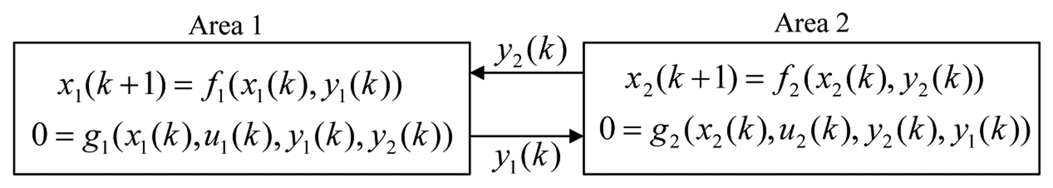
Figure 6 shows a simple, but prototypical, multi-area power network composed of only two interacting areas. The behavior of each area is effectively represented by the difference-algebraic equations, ignoring the discrete-event state variables, for simplicity. The areas physically interact via infinitely fast-changing algebraic state variables, i.e., y1 and y2 (voltage/current or active/reactive powers over the tie-lines).
Considering Area 1 as an example and assuming that the Jacobian of g1 with respect to is non-singular, one can obtain the control action, u1, at time tk as a function of the other variables:
Equation (1) shows the effect of interaction variable from Area 2 (y2) on the control action of Area 1 (u1). Similarly, for y2:
Substituting Equation (2) in Equation (1) clearly shows how u2 can affect u1.
In the current implementation of the DCMPC approach in this article, we have taken this effect into account by providing to CA1 (corresponding to Area 1) the optimal control sequence of CA2 (corresponding to Area 2), , over a prediction horizon, H, i.e.,
This seems to be an effective signal to be communicated, as the simulation results show that the uncoordinated local control actions can lead to voltage collapse. The exchange of the information of the planned control sequences allows each CA to “actively/directly” take its own coordinated local control actions, knowing what the neighbors are planning to do.
Another possible signal to be exchanged, instead of exchanging the planned control sequences, might be the exchange of the planned output trajectories of interacting variables directly (e.g., the expected values of future voltages over the tie-lines), i.e.,
However, this seems to be much too complex, as the neighbors will “passively/indirectly” coordinate. Each CA is then expected to try to take into account the voltage profile of its neighbors by taking some local control actions and without knowing what the neighbors themselves will do in the future in order to correct their (potential) voltage violation. This might mislead the neighbors and stop them from reacting. This, in turn, can at least lead to a slower correction of a low voltage condition, assuming that the potential misunderstandings among neighbors can be resolved after some iteration of information exchange.
3.6. Computational Burden
One should clearly distinguish between the local control models and the physical model of the overall system. There exist several local discrete time control models, one for each area, in order to enable the local MPC of each CA to perform its iterative finite-horizon optimization at each discrete time instant. These local control models obviously differ from one CA to another. However, on top of this, there also exists one continuous model for the overall physical power system (with information available from all areas) in order to simulate the dynamic response of the physical power system after applying the control actions calculated by the local MPCs. In other words, the DCMPC requires all local MPCs to concurrently calculate the local control actions for each time instant, say tk, by using the distinct discrete time local control models of their own area, reduced-order models of their immediate neighbors and for the distant areas. It then applies all these calculated control actions to the physical system in continuous real time, and lets the overall system evolve until the next time instant, in this case, tk+1. At tk+1, all the state variables will be collected by performing new (noisy) measurements in the real physical power system, which will indeed be used as initial conditions for solving the local optimization problems by the local MPCs at tk+1. This procedure is identically repeated for all following time instants. Thus, the CPU time required to complete a simulation experiment consists of two distinct terms: the time that the local MPCs take to calculate their optimal control actions at each discrete time instant, plus the time needed to simulate the physical system after applying these calculated control actions in order to obtain the state variables at the end of that control interval. In order to determine whether or not the DCMPC algorithm is suitable for real-time applications, what matters is the time needed for computing the local control actions for each CA (and not for all CAs) and, obviously, not for the simulation of the physical system. The DCMPC requires each CA to perform a number of simulation runs, i.e., one simulation run per each possible control sequence, in order to select the best local sequence in a reasonably short CPU time.
For the Nordic32 test system, the slowest agent-wise simulator time for solving the local optimization problem, using a variable step size solver, when running on a Windows PC with 3.154 GHz Intel Core 2 Duo CPU and 4 GB of RAM, was less than 3 s. Taking into account that each CA makes decisions at every 10 s, this ensures that the approach can meet the requirement for on-line voltage control.
Regarding why simulation stops and cannot proceed at the time of voltage collapse, first of all, due to step size reduction limitations, the simulation stops when the trajectory of the system variables changes too fast, as occurs during a voltage collapse. Moreover, the solver may not be able to find a solution to algebraic equations at the time of voltage collapse.
Recall that the hybrid nonlinear dynamic behavior of power systems involves an intrinsic strong coupling between continuous dynamics and discrete events. This occurs, for example, during voltage collapse phenomena, when several discrete devices (either discrete controllers, like LTCs or capacitor banks, or thresholds influencing continuous dynamics, like OXL) switch on and off as a reaction to local measurements of currents and voltages that are influenced by local and global continuous dynamics of the network.
To deal with this, as explained in Section 3.2., we have intentionally employed a hybrid modeling framework to formulate the long-term voltage coordination problem in Modelica (an object-oriented equation-based language to model complex physical systems), using Dymola (a tool for modeling and simulation of integrated and complex systems). Our hybrid Modelica models are described by a set of DAEs and discrete events. This hybrid nature leads to a mixed continuous/discrete system of equations at event instants that have to be solved by appropriate algorithms. Furthermore, different solvers may be used to determine the next simulation time (current simulation time plus step size) at which the set of DAEs, represented by the mathematical model of the system, should be solved. The difference between the true analytical solution and the computed approximated solution by numerical integration is defined as the local error. Generally, decreasing the step size increases accuracy, as well as simulation time, and vice versa.
We have employed the variable-step solver of Dymola, which dynamically adjusts the step size during the simulation depending on the model dynamics and provides error control. Thus, by using local error, the solver reduces the step size to increase accuracy when a model's states are changing rapidly and increases the step size to avoid taking unnecessary steps when the model's states are changing slowly. The general effect will be that, for a given level of accuracy, the total number of steps will be reduced and, thus, overall simulation time, required to maintain a specified level of accuracy for models with rapidly changing or piecewise continuous states, will also be significantly reduced.
This indeed explains the behavior of the system when simulation stops and cannot proceed. When fast changes in voltage occur during collapse (which is the ultimate result of the activation of some OXLs, LTCs and their interactions), the solver tries to reduce the step size in order to maintain the required accuracy. However, since fast changes are so big that the required accuracy cannot be maintained, the solver fails to find a set of solutions and expectedly stops.
4. Results with the Uncoordinated Decentralized MPC
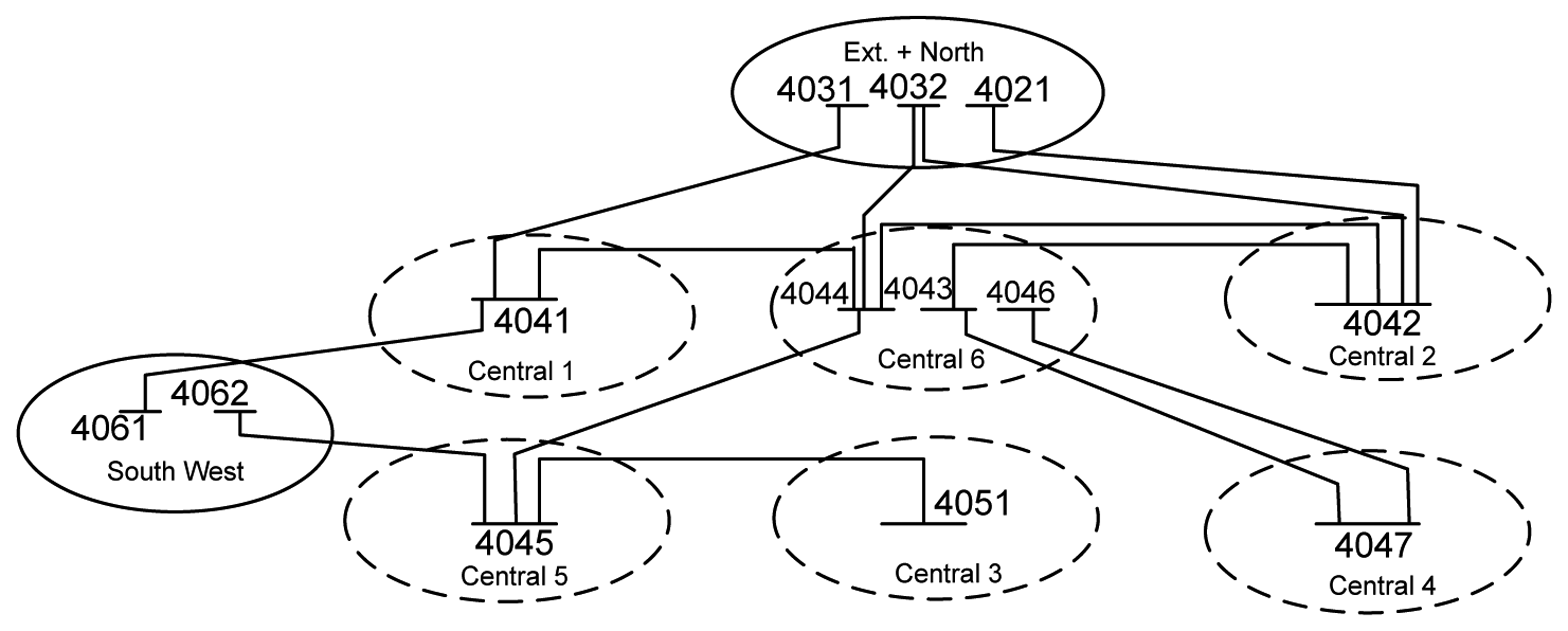
It is of interest in this article to find out what is the contribution of combining anticipation and coordination to improved performance of the DCMPC. The authors of [5] compare the good performance of the DCMPC approach with the uncoordinated decentralized deadband control of LTCs, illustrating the joint contribution of the anticipation and coordination feature of the DCMPC. This article, in order to find out the sole contribution of coordination, compares the results presented in [5] with the uncoordinated decentralized MPC approach, under identical disturbances. We consider two disturbances, on a slightly modified version of the CIGRENordic32 test system [17]. A one-line diagram of the decomposed Nordic32 is shown in Figure 7.
Note that the control objective of each CA is two-fold. The main objective of CAi, i ∈ {1,…, M} is to maintain at time t its Bi voltage magnitudes at buses B ∈ {1,…, Bi} within prescribed bounds close to the nominal bus voltages. In this paper, we consider puand pu for all CAs. A simple quadratic cost is employed to penalize the voltage deviations for the buses. The secondary objective is to minimize the number of changes of tap positions in its Li LTCs L ∈ {1,…, Li}, as they cause transients on the system voltages, as well as mechanical wear on the LTCs themselves.
4.1. Case 1: Outage of Lines 4032–4044
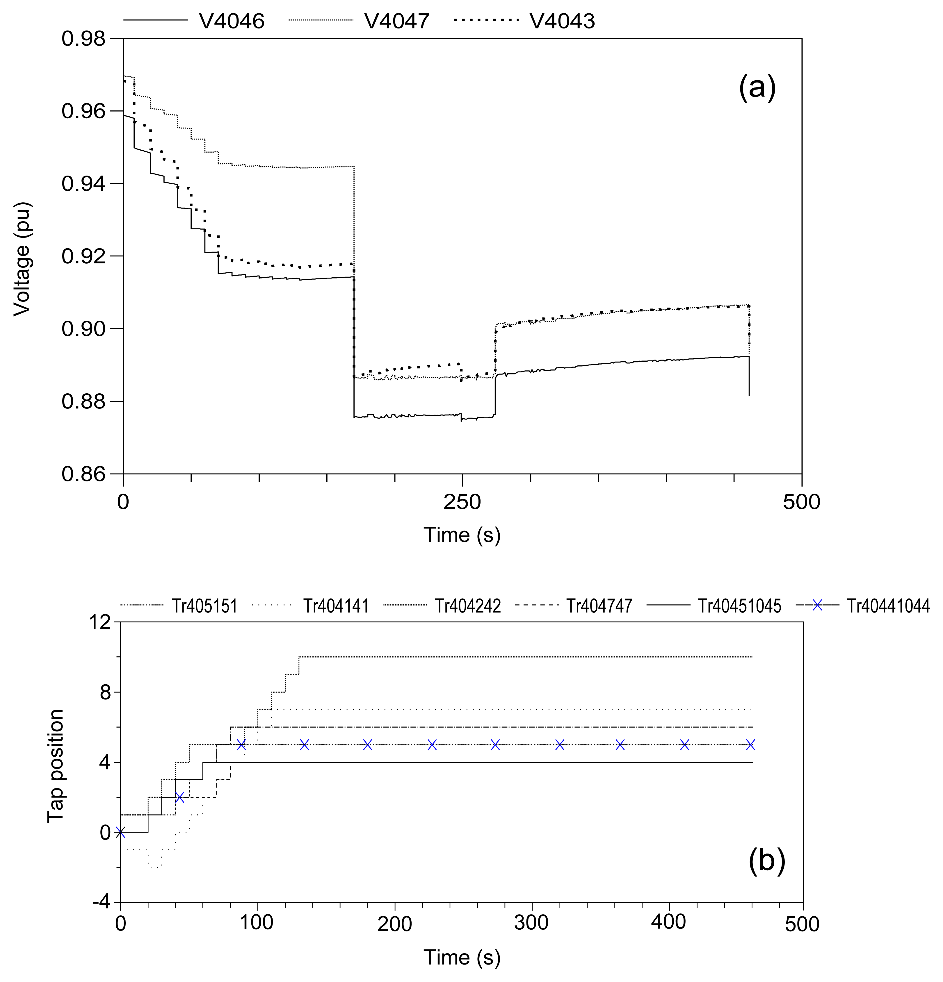
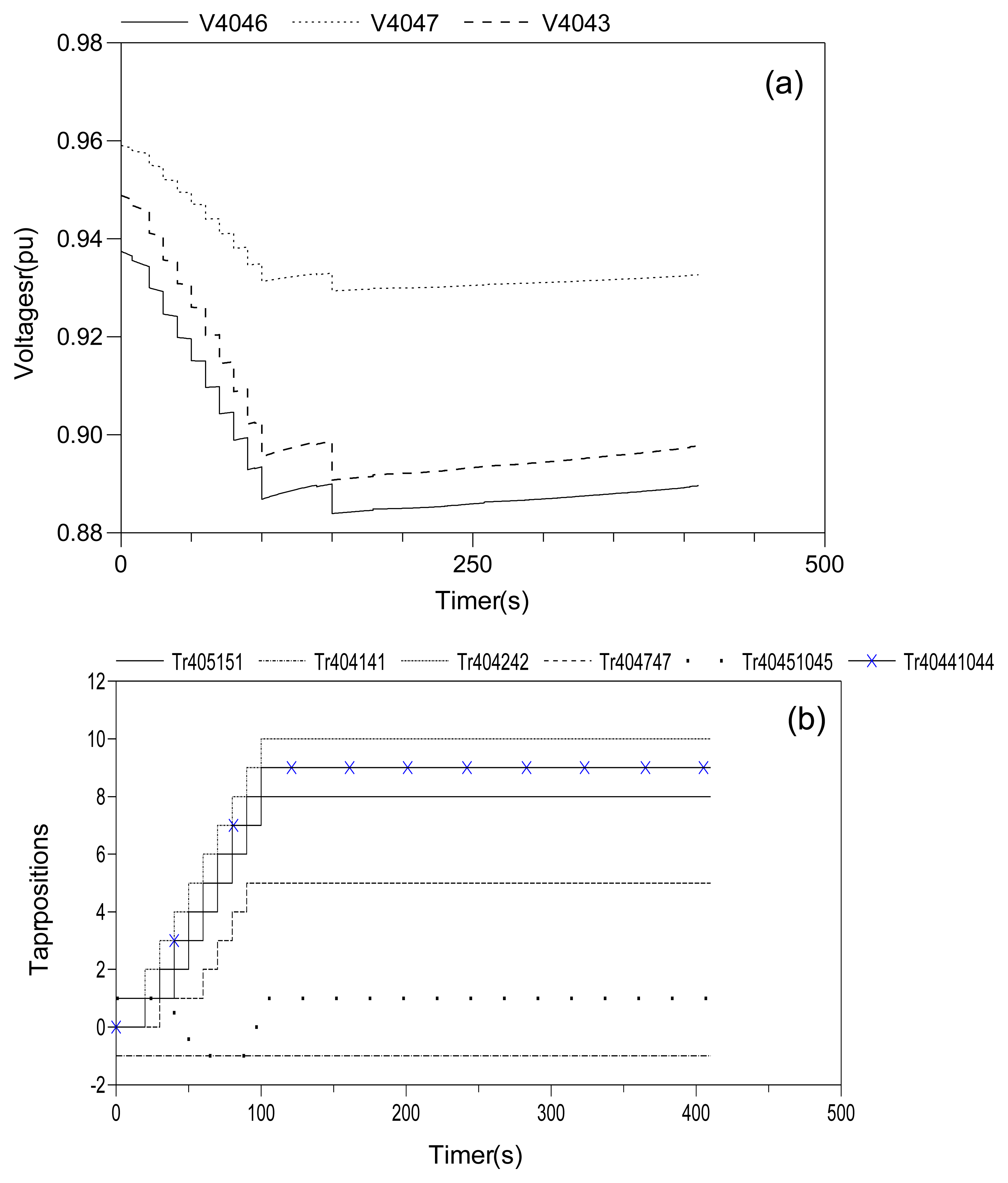
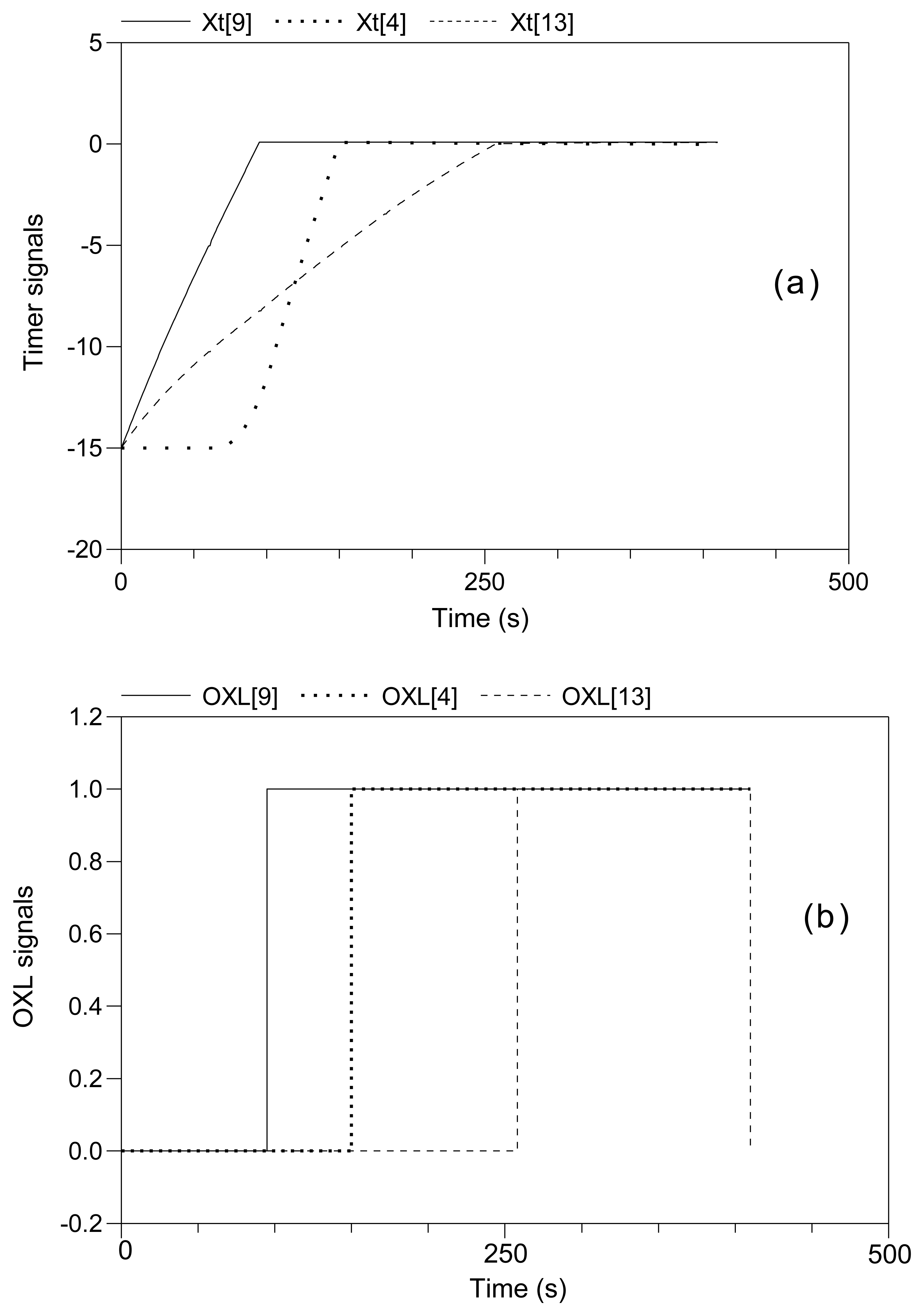
Figure 8 shows the voltage evolution at Buses 4046, 4047 and 4043, which, controlled according to decentralized MPC, experience the largest drop, when the local MPCs receive no information from their neighbors, and assume that the neighbors will take no control action. The overall system survives until t = 461 s, when simulations stop, lasting some 235 s longer than that with decentralized deadband control. This uncoordinated decentralized MPC approach, as shown in Figure 9, leads to the activation of OXLs over three machines, g13, g15 and g17, at t = 170, 274 and 459.8 s, respectively.
In comparison to the decentralized deadband control, only LTC Tr404242 in Central2 reaches its maximum tap limit, while three other LTCs, namely Tr404141 in Central1, Tr405151 in Central3 and Tr404747 in Central4, have not moved toward reaching their limits, thanks to the local MPC's anticipation. Furthermore, at t = 50 s, the local MPC for Central2 successfully anticipates moving towards activation of OXL for g13 and, therefore, freezes the upward tap movements of the local LTC Tr404242 for three subsequent steps. However, due to the lack of coordination with the actions of the neighbors, eventually, g13 becomes limited. Likewise, Central4 fails at preventing the activation of OXL over g15.
4.2. Case 2: Outage of Lines 4011–4021
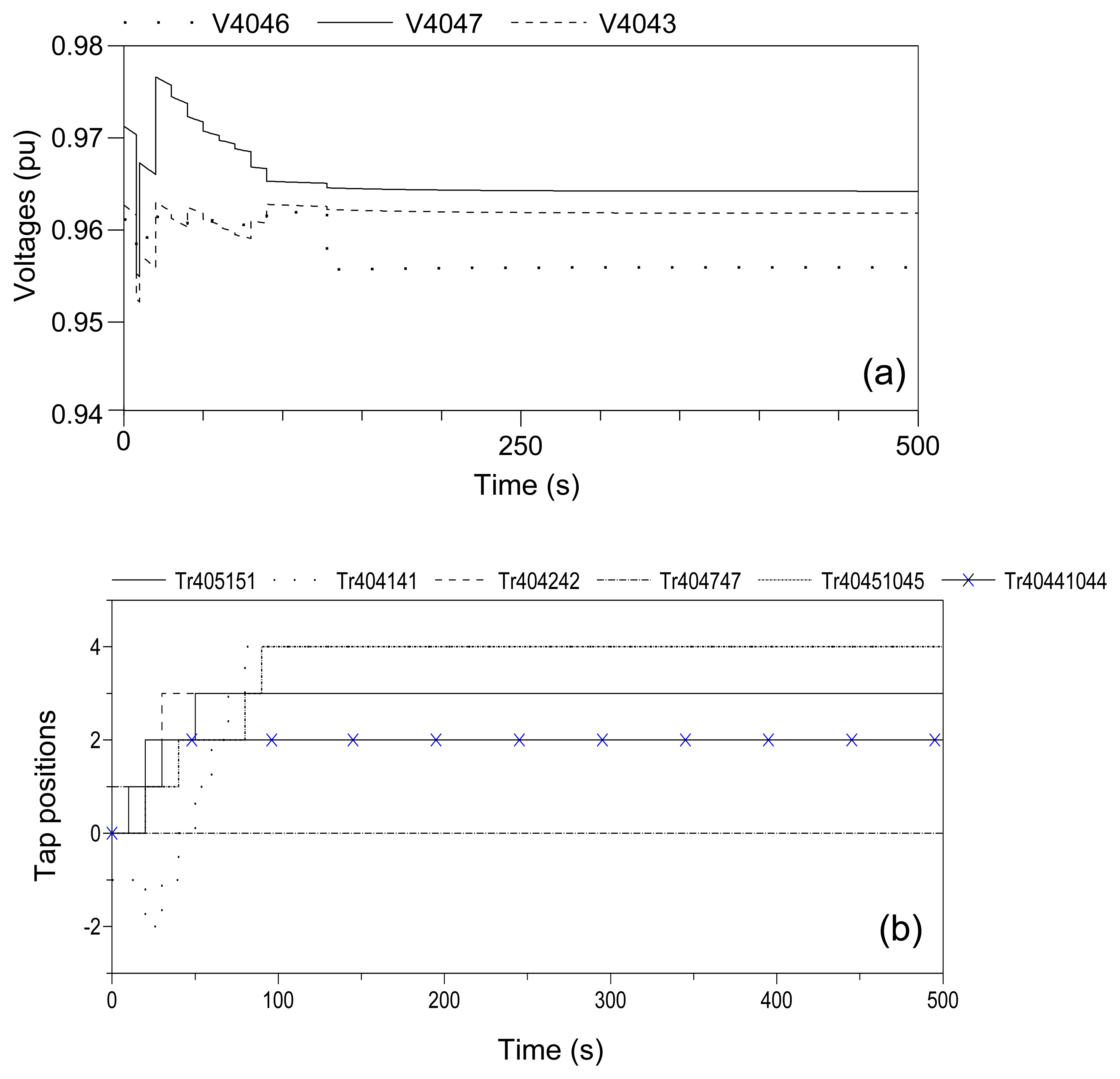
Figure 10 shows the voltage at Buses 4046, 4047 and 4043, as well as the decentrally calculated uncoordinated local MPC control actions. The system manages to survive the disturbance until t = 410 s, when the numerical integration cannot proceed further, lasting some 121 s longer than under the deadband control of the LTCs. As shown in Figure 11, only three OXLs are activated over machines g9, g4 and g13 at t = 95, 150 and 258 s, respectively. This is thanks to the local anticipating feature of the MPCs in solving their own greedy local optimization problem. Note that only one LTC, namely Tr404242 in Central2, still reaches its limit at t = 100 s, withdrawing voltage support that could relieve the local generator, g13, of final saturation.
5. Robustness Analysis
In the simulations presented so far for the Nordic32 test system, the reduced-order QSS models for the immediate neighboring areas, as well as the PV models for the distant areas are assumed to be correctly given for each local area. It is of interest to perform additional experiments to assess the robustness of the DCMPC against modeling errors and to test the impact of the unmodeled dynamics of the neighbors. To this end, the consumed active power of the LTC-controlled load at Bus 4043 in Central6, the most critical area with the most immediate neighbors containing three LTCs represented by a single equivalent one, is increased by 10% at t = 0 s for the simulation of the physical system. However the models used by neighboring CAs (Central1, Central2, Central4 and Central5) for anticipating the power flows along the transmission lines connecting them to Central6 are not updated at t = 0 s. Figure 12 shows the evolution of voltages at buses under the effect of the same disturbance as in Case 1 (i.e., the outage of Lines 4032–4044 at t = 10 s and, in addition, all other neighbors assuming the wrong parameter value for the load at Bus 4043 in Central6 at t = 0 s.
The bus voltages are quite similar to (but lower than) those of the base disturbance in Case 1, all stabilized within the limits in the long term. However, in response to initiating (at t = 0 s) a “disturbance-like” load change in Central6, the local LTC, Tr40441044, advances its upward tap move (from t = 20 s in the base disturbance) to t = 10 s, continued by another upward tap move at t = 20 s in response to the line outage at t = 10 s. Furthermore, the neighboring LTC, Tr4047, in Central4 reacts to the nearby load change by taking a downward tap move at t = 20 s, and LTC Tr4042 in Central2 changes its (original base disturbance) LTC moves by freezing its upward moves at t = 30 s (instead of t = 40 s). The other neighbors do not change their LTC moves at all by properly coordinating them with this new set of control actions taken by the CAs in Central6, Central4 and Central2.
6. Towards Practical Implementation
This article and [5,10] have shown that the DCMPC is a feasible approach to reduce the risk of voltage collapse in a real system by studying some well-known case studies. One should notice that the DCMPC scheme complements (and does not replace) the existing secondary control layer of a generic voltage control hierarchy. It essentially equips each CA with an anticipation feature and provides an additional feedback coordinating signal among LTCs. This makes the DCMPC approach incrementally implementable in practice, meaning that, considering the ENTSO-E grid, for example, the entire 41 TSOs (and their underlying CAs) do not necessarily need to change their current voltage control strategy for LTCs at once. The fact that the DCMPC implementation can begin from one single TSO would then make it possible to have a configuration in which a DCMPC-controlled CA might have some neighbors using another strategy, e.g., deadband-controlled neighboring CAs. This will not cause any problem, because as long as the DCMPC-controlled CA is informed, by some limited amount of communication, about the (one-step-ahead) control actions of its (even still possibly deadband-controlled) CAs, it will effectively take this information into account for calculating its own coordinated control actions.
A (potential) improvement for realizing practical applications might be achieved by the asynchronous implementation of the DCMPC. This may possibly provide an even more realistic operation of CAs by allowing them (in general) to update their control actions whenever they want to. In this way, the local CAs can base their decisions on more recent control plans from their neighbors than the previous synchronous time instant. However, due to the mechanical time delay of LTCs, the CAs would then still use the same control interval of 10 s, but could start reacting at different times within each 10-s interval.
It is also important to mention that the multi-area power systems are often heterogeneous networks stretching out over many independent TSOs (and their corresponding CAs) in different countries. Thus, the possible non-cooperative behavior of some CAs (or even preventing a malicious operator from actually damaging the overall system) must be rewarded, enforcing cooperation in practice. However, we do not deal with this issue, assuming that the TSOs adhere to their contract, which forces them to cooperate for the proposed DCMPC scheme.
7. Extension of the DCMPC
In this article, at most, one LTC (except area Central6 containing three LTCs) is considered for each area. A control horizon of 30 s (N = 3) is chosen to perform the simulations. Each MPC, corresponding to each CA, enumerates the number of all possible LTC move sequences without excluding those that the designer knows in advance will almost certainly not be optimal. This may be an issue, in terms of computational complexity and simulation time, when the size of the system grows or when longer control horizons are considered. Therefore, additional work is required to reduce the number of possible input sequences, based on some heuristics and on physical intuition.
In the current implementation, each CA knows a detailed local model of its own area, as well as reduced-order QSS models of its immediate neighboring areas, assuming simpler equivalent PV model for the distant areas. Future works can be devoted to devising abstraction methods to dynamically represent a more abstract model of the neighboring areas. The abstract models may not necessarily have the same degree of accuracy and details compared to that of local areas.
This article does not consider the power-flow constraints of interconnecting tie-lines. These constraint are due to the thermal limits of tie-lines, which can, in turn, limit the maximum cross-border power interchange among areas. This additional constraint should also be taken into account in the future implementations of the DCMPC.
The DCMPC coordination scheme may also be applied as a tool for designing coordinated controllers for microgrids (μ-grids), including DGsand storage devices. Analogous to the proposed DCMPC concept, a multi-area small-scale power system can be determined, within the microgrid, by considering, for example, each feeder as an area and assigning a local MPC to it. These decomposed areas, or feeders, are sometimes referred to as “active cells”. However, due to the fundamental X/R ratio difference between transmission and distribution networks, an effective coordinated voltage control design for smart grids, besides LTC controls, should consider the control of storage and of deferrable loads, as well. Smart grid control in long time scale is an economic dispatch problem that can be effectively tackled by the proposed coordination paradigm. In this case, the communication may include the variable import/export electricity pricing among cells, over a prediction horizon in the future.
8. Conclusions
The proposed DCMPC approach is a novel communication-based control architecture for LTCs in order to improve the coordination among the corresponding CAs. This coordinating feedback controller acts in the time scale of 10 s and, thus, is suitable for mitigating the long-term voltage decays. Simulation results presented in this paper and [5] illustrate the improved performance of the DCMPC-controlled LTCs in comparison to a deadband and MPC-based decentralized control of LTCs. Thanks to the joint contribution of the anticipation and coordination features of the DCMPC, the decentralized MPC scheme exhibits an intermediate performance, due to lack of coordination with neighbors. The LTCs under traditional deadband control exhibit the lowest performance, due to the lack of both anticipation and coordination features of the DCMPC. Each CA knows a detailed local model of its own area, as well as reduced-order models of its immediate neighboring CAs, assuming simpler equivalent models for the remote areas. The practical implementation issues and the feasibility of the approach for real-time voltage control has been elaborated in an attempt to convince practitioners to consider the DCMPC approach as a feasible scheme to reduce the risk of blackouts. However, additional work is needed in order to further ascertain the viability of the DCMPC as an advanced control approach for mitigating the long-term voltage instability.
Acknowledgments
The research was carried out in the frame of the Inter-university Attraction Poles program IAP-VII-02, funded by the Belgian Government.
Conflicts of Interest
The authors declare no conflict of interest.
References
- Amin, M. North American Electricity Infrastructure: System Security, Quality, Reliability, Availability, and Efficiency Challenges and Their Societal Impacts; University of Minnesota: Minneapolis, MN, USA; June; 2004. [Google Scholar]
- Mousavi, O.; Cherkaoui, R. Literature Survey on Fundamental Issues of Voltage and Reactive Power Control; École Polytechnique Fédérale de Lausanne: Lausanne, Switzerland, 2011. [Google Scholar]
- Jin, L.; Kumar, R. Security Constrained Coordinated Dynamic Voltage Stabilization Based on Model Predictive Control. Proceedings of the IEEE Power & Energy Society General Meeting, Calgary, AB, Canada, 26–30 July 2009; pp. 3979–3986.
- Union for the Co-Ordination of Transmission of Electricity (UCTE). Final Report on System Disturbance on 4 November 2006; Technical Report; UCTE: Brussels, Belgium; January; 2007. [Google Scholar]
- Moradzadeh, M.; Boel, R.; Vandevelde, L. Voltage coordination in multi-area power systems via distributed model predictive control. IEEE Trans. Power Syst. 2013, 28, 513–521. [Google Scholar]
- Moradzadeh, M.; Boel, R. A Hybrid Framework for Coordinated Voltage Control of Power Systems. Proceedings of the International Power & Energy Conference (IPEC), Singapore, 27–29 October 2010; pp. 304–309.
- Van Cutsem, T.; Vournas, C. Voltage Stability of Electric Power Systems; Springer US: New York, NY, USA, 1998. [Google Scholar]
- Larsson, M.; Karlsson, D. Coordinated Control of Cascaded Tap Changers in a Radial Distribution Network. Proceedings of the Stockholm Power Tech Conference, Stockholm, Sweden, 18–22 June 1995; pp. 686–691.
- Shan, J.; Annakkage, U.D.; Gole, A.M. A platform for validation of FACTS models. IEEE Trans. Power Deliv. 2006, 21, 484–491. [Google Scholar]
- Moradzadeh, M.; Bhojwani, L.; Boel, R. Coordinated Voltage Control via Distributed Model Predictive Control. Proceedings of the Chinese Control and Decision Conference, Mianyang, China, 23–25 May 2011; pp. 1612–1618.
- Phulpin, Y.; Begovic, M.; Petit, M.; Heyberger, J.-B.; Ernst, D. Evaluation of network equivalents for voltage optimization in multi-area power systems. IEEE Trans. Power Syst. 2009, 24, 729–743. [Google Scholar]
- Hug-Glanzmann, G.; Andersson, G. Decentralized optimal power flow control for overlapping areas in power systems. IEEE Trans. Power Syst. 2009, 24, 327–336. [Google Scholar]
- Modelica Association. Available online: https://www.modelica.org/ (accessed on 19 November 2013).
- Van der Schaft, A.J.; Schumacher, H. Introduction to Hybrid Dynamical Systems; Springer: Berlin, Germany, 1999. [Google Scholar]
- Capitanescu, F.; Otomega, B.; Lefebvre, H.; Sermanson, V.; van Cutsem, T. Decentralized tap changer blocking and load shedding against voltage instability: Prospective tests on the RTE system. Int. J. Electr. Power Energy Syst. 2009, 31, 570–576. [Google Scholar]
- Otomega, B.; Sermanson, V.; van Cutsem, T. Reverse-Logic Control of Load Tap Changers in Emergency Voltage Conditions. Proceedings of the Bologna Power Tech Conference, Bologna, Italy, 23–26 June 2003.
- Long-Term Dynamics-Phase II; CIGRE Task Force: Paris, France, 1995.
Acronyms
| CA | control agent |
| MPC | model predictive control |
| TSO | transmission system operator |
| QSS | quasi steady-state |
| DCMPC | distributed communication-based model predictive control |
| LTC | load tap changing transformer |
| OXL | over excitation limiter |
| HA | hybrid automaton |
| DAE | differential-algebraic equation |


© 2014 by the authors; licensee MDPI, Basel, Switzerland. This article is an open access article distributed under the terms and conditions of the Creative Commons Attribution license ( http://creativecommons.org/licenses/by/3.0/).
Share and Cite
Moradzadeh, M.; Boel, R.; Vandevelde, L. Anticipating and Coordinating Voltage Control for Interconnected Power Systems. Energies 2014, 7, 1027-1047. https://doi.org/10.3390/en7021027
Moradzadeh M, Boel R, Vandevelde L. Anticipating and Coordinating Voltage Control for Interconnected Power Systems. Energies. 2014; 7(2):1027-1047. https://doi.org/10.3390/en7021027
Chicago/Turabian StyleMoradzadeh, Mohammad, René Boel, and Lieven Vandevelde. 2014. "Anticipating and Coordinating Voltage Control for Interconnected Power Systems" Energies 7, no. 2: 1027-1047. https://doi.org/10.3390/en7021027