Modelling of PEM Fuel Cell Performance: Steady-State and Dynamic Experimental Validation

Abstract
: This paper reports on the modelling of a commercial 1.2 kW proton exchange membrane fuel cell (PEMFC), based on interrelated electrical and thermal models. The electrical model proposed is based on the integration of the thermodynamic and electrochemical phenomena taking place in the FC whilst the thermal model is established from the FC thermal energy balance. The combination of both models makes it possible to predict the FC voltage, based on the current demanded and the ambient temperature. Furthermore, an experimental characterization is conducted and the parameters for the models associated with the FC electrical and thermal performance are obtained. The models are implemented in Matlab Simulink and validated in a number of operating environments, for steady-state and dynamic modes alike. In turn, the FC models are validated in an actual microgrid operating environment, through the series connection of 4 PEMFC. The simulations of the models precisely and accurately reproduce the FC electrical and thermal performance.1. Introduction
Fuel cells (FC) have received a major boost in recent years, as a result of the growing demand by a number of sectors. For this reason, this technology is rapidly expanding and there are many different research lines associated with the various sectors. There are basically three sectors behind the development of fuel cells: namely, the transport sector [1,2], the portable device sector [3] and the stationary application sector [4]. Within the stationary sector, particular mention should be given to the integration of hydrogen-based storage systems with renewable energies. The main advantage of these systems compared to other storage technologies is the fact that they are able to store energy for a long period of time, making it possible to better deal with the seasonal variability of the renewable resources [5]. The feasibility of renewable energy based hydrogen production, and its subsequent utilization to generate electricity through the use of FCs has been widely demonstrated in a number of research projects and papers [6–9]. Over the last few years, a particular case which has excited much interest is the integration of hydrogen based fuel storage systems with renewable energies in microgrid applications [10–14].
A wide range of FC technologies are available, which are at different stages of development. Although FCs can be classified into a number of categories, based on the type of fuel used (such as hydrogen, methanol or natural gas), the operating temperature (ranging from ambient temperature up to 1000 °C), FCs are generally classified according to the type of electrolyte. However, regardless of the FC technology used, in all cases the net reaction for the recombination of hydrogen and oxygen to form water, is the same [15]. The principal FC technologies, based on the electrolyte used, are: proton exchange membrane (PEMFC), this type includes direct methanol (DMFC), alkaline (AFC), phosphoric acid (PAFC), molten carbonate (MCFC) and solid oxides (SOFC). The PAFC, MCFC and SOFC operate at high temperatures, 220 °C, 650 °C and up to 1000 °C, respectively, whereas the AFC operating temperature may vary from 50 to 200 °C, offering a higher performance than the PEMFC, however in that case the hydrogen and oxygen must be pure for optimal performance [16].
The PEMFCs operate at a lower temperature, generally under 100 °C and, therefore, the connection time is faster than for other FC types. In turn, they show a rapid response to load variations, and are also compact, lightweight, noiseless and, furthermore, as they use a solid polymer electrolyte, they are easier to manufacture than other FC types, such as the AFCs. The PEMFCs have been validated in a number of applications such as automobiles, buses, distributed generation, cogeneration, stand-alone systems and portable systems [17].
The scientific literature contains a number of papers on FC modelling, including theoretical and empirical models, some of which model the FC whilst others are focused on the different FC components such as electrodes, membrane, etc. [18,19].
The modelling of the FC electrical performance can be classified according to the FC operating mode. Some authors propose steady-state models which analyse the operation of the FC at either a fixed operating point or with slow dynamics [20–26] whilst other authors have developed dynamic models to analyse the operation of the FC in transient modes. With regard to the dynamic electrical models published in the literature, most authors associate the FC dynamic performance with the double layer effect. In general, the double layer effect is modelled with a capacitor in parallel to the equivalent resistor, due to the activation and/or concentration phenomena [27,28]. With regard to the concentration effects, which are principally influenced by diffusion, some authors use the Warburg impedance for modelling purposes [29–31]. In order to obtain the FC dynamic model, a number of experimental methods are available [15,28], such as a study of the voltage step response in relation to the current step up demanded from the FCs [32–34]. However, the results are more accurate using the electrochemical impedance spectroscopy (EIS) technique [27,29,30,35,36]. Likewise, the literature includes models that combine the electrical performance in the steady-state and dynamic modes. In these models, some authors take account of the losses derived from the concentration phenomena, such as Wingelaar et al. [37], who models a 500 W FC, although no consideration is given to the influence of the temperature on the experimentally obtained parameters. Furthermore, other authors model the concentration overvoltage using an empirical expression [38,39] whilst others, such as Ferrero et al. [40] solely consider the said overvoltage for the steady-state model and not for the dynamic one.
On the other hand, a number of authors have worked on the FC thermal modelling, proposing semi-empirical models based on thermal balance that are valid for steady-state and dynamic modes [41,42]. These models are based on a thermal energy balance. Some authors calculate the heat dissipated by forced convection through the heat exchange surface area and the mean logarithmic temperature [43,44]. Others authors experimentally calculate the FC overall heat transfer coefficient in order to account for the variation in cooling based on the current demanded [45]. Likewise, other authors calculate the forced convection coefficient through an experimental expression depending on the FC fan control signal [38,46]. However, other authors analyse the convection mechanisms in greater detail, establishing empirical relationships in order to determine the convection coefficients [47–49]. Whilst other authors are focusing their research on determining a model which describes the influence of the hydrogen purges on the FC operation [50].
With regard to the modelling of the various FC components, some authors have developed in-depth models focused on phenomena occurring in the said components, such as the transport of water [51–54] or reactants [55], at the diffusion layer and the electrodes alike. Other authors focus on the porosity of the electrodes through macroscopic studies [56–58]. All this research work is of great interest, in order to improve the various FC components.
This article reports on the modelling of a commercial 1.2 kW PEMFC configured through an electrical model and a thermal model, able to represent its performance in any operating regime. Firstly, an electrical model is proposed, based on the integration of the different thermodynamic and electrochemical phenomena taking place in the FC. This model predicts the FC voltage for a steady-state and dynamic mode alike. A thermal model is then developed, based on the FC thermal energy balance, capable of predicting the FC operating temperature in relation to the ambient temperature. Once the models have been established, the next step is to characterise and obtain the parameters associated with the electrical and thermal performance. Then the models representing the FC electrical and thermal performance are implemented in Matlab Simulink and are validated in a number of steady-state and dynamic operating environments. Finally, the models are validated in an actual operating environment through the integration of four PEMFCs in the microgrid located in the Public University of Navarra (UPNa).
2. Experimental Setup
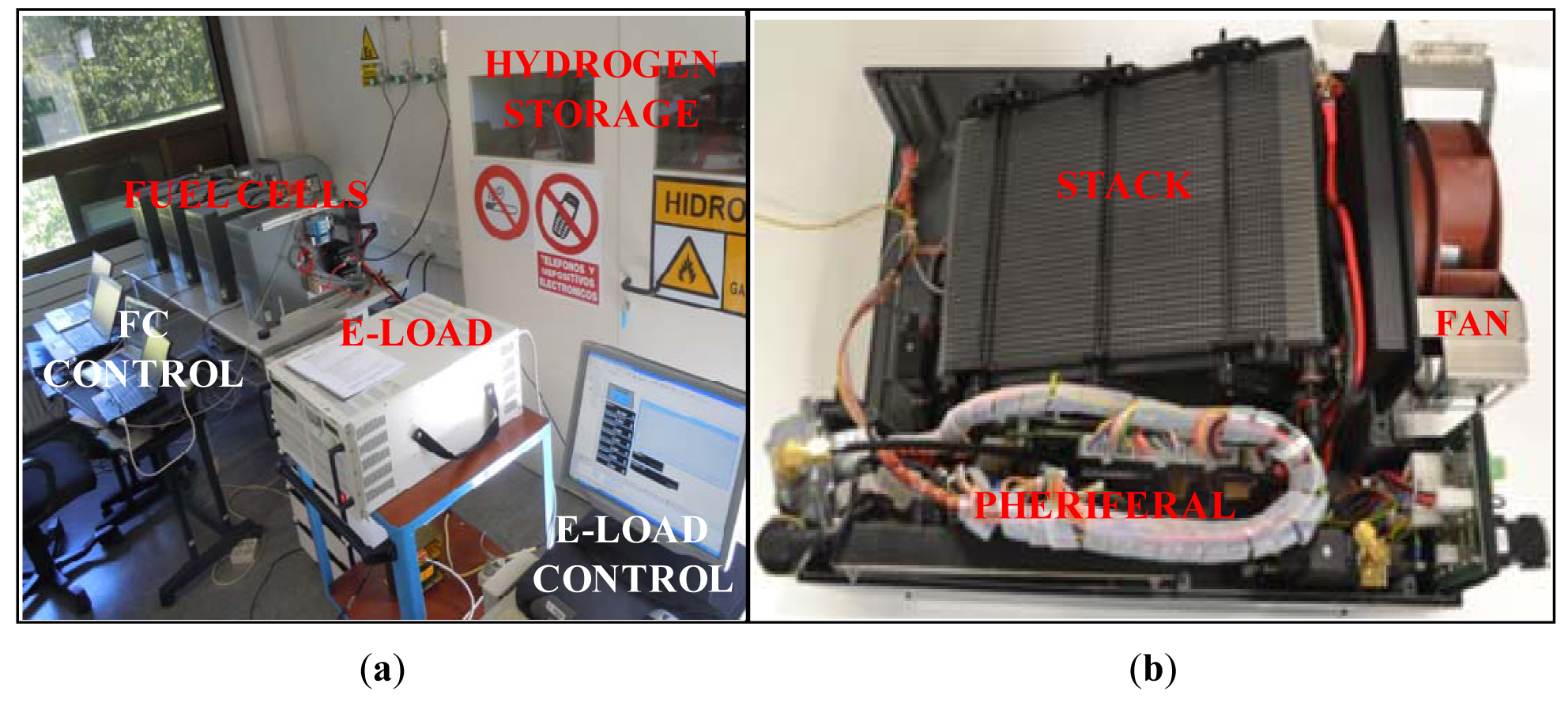
The FC experimental study was conducted at the UPNa Renewable Energies Laboratory. The laboratory, shown in Figure 1a, is equipped with a hydrogen system comprising four FCs and a hydrogen supply system. Furthermore, there are plans to install a PEM water electrolyser. The hydrogen supply system comprised four hydrogen B50 cylinders, with a total capacity of 35.2 Nm3. The four PEMFCs are identical, corresponding to model NEXA1200, supplied by Heliocentris (Berlin, Germany). This FC model obtains oxygen from the air and has a power output of 1200 W, with heat and water vapour being its only by-products. Figure 1b shows a photo of the interior of one of the FCs, where it is possible to see the stack, fan and internal FC peripherals such as the control board and purge valve. Each FC comprises a Ballard stack of 36 series-connected cells with a surface area of 145 cm2. According to the manufacturer's specifications the voltage range is 20–36 V and the maximum current is 60 A. The maximum FC operating temperature is 65 °C and it is equipped with a pressure regulator to maintain the hydrogen operating pressure in the stack at around 1.32 bar (absolute pressure). Likewise, each FC has an external hydrogen solenoid valve, a sensor to measure the hydrogen flow rate, an external power supply to power the FC at start-up and software to start and stop the FC and to obtain the principal operating variables (FC CONTROL). In addition, it incorporates a relay and a diode to prevent damage to the system when the FC is connected to the load. The sensor used to measure the hydrogen flow rate is model GSEM C9TS DN00 of red-y smart series made by Vögtlin Instruments (Aesch, Switzerland).
Furthermore, the laboratory is equipped with other equipment to perform the various experiments required for this present work: namely a programmable electronic load (E-LOAD), shown in Figure 1a, and a frequency response analyzer (FRA), both devices being made by AMREL (American Reliance Programmable Power, San Diego, CA, USA)). The electronic load has an operating range from 0 W to 7500 W, with a maximum voltage and current input of 600 V and 400 A respectively. The load is programmed through a digital signal processor (DSP) housed in a PC (E-LOAD CONTROL). In this way, the FC modelling and characterisation tests are programmed, in addition to the current and power profiles to be supplied by the FCs in the different operating environments. The frequency response analyser has a frequency range of up to 20 kHz. This is used in combination with the electronic load in order to perform the EIS tests on the FCs. The laboratory also has a range of instruments to measure the electrical quantities analysed, such as a four-channel YOKOWAGA WT1600 Meter (Yokowaga Electric Corporation, Tokyo, Japan) and a model TDS 5034 digital oscilloscope (Tektronix, Beaverton, OR, USA).
3. Modelling
3.1. General Points
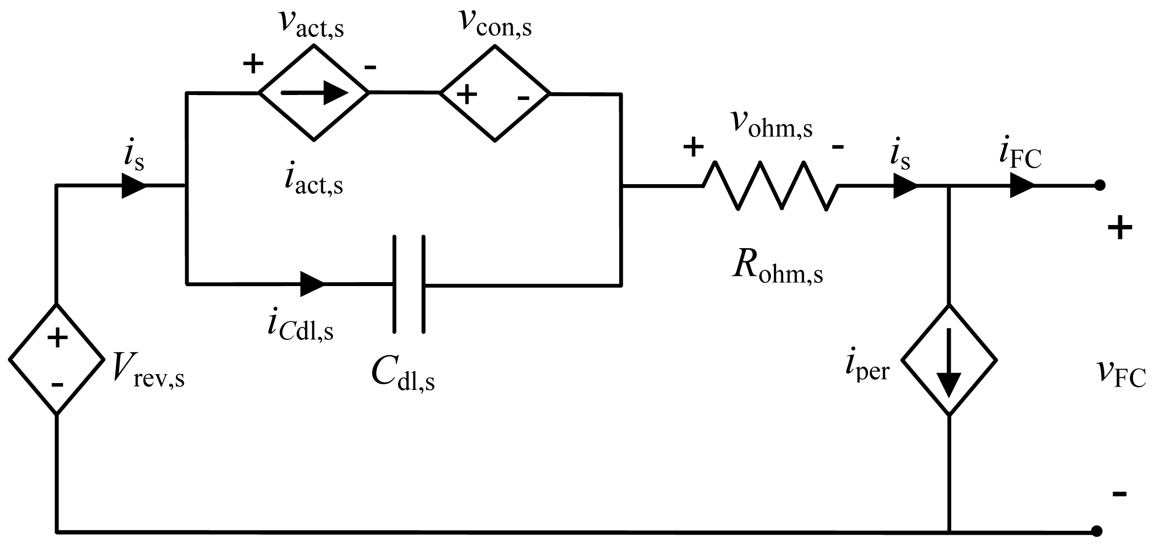
This subsection deals with the modelling of one of the FCs described in Section 2. The modelling developed is configured through an electrical model and a thermal model. The combination of both models predicts the FC electrical and thermal performance. Figure 2 shows the model representing the FC electrical performance, in steady-state and dynamic modes. The electrical model comprises a number of elements which represent the thermodynamic and electrochemical phenomena occurring in the FC, as well as the consumption of the peripherals. This model reproduces the FC electrical performance, based on the current demanded and the FC operating temperature, as described in Subsection 3.2.
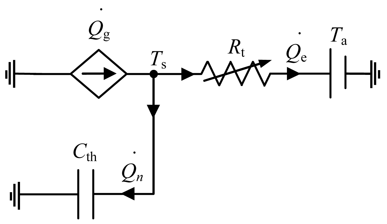
Temperature is a determining factor in the FC electrical performance, the FC electrical variables shown in Figure 2 are dependant on the FC operating temperature. For this reason, in Subsection 3.3 the FC thermal model is developed. The thermal model is shown in Figure 3 and comprises the electrical elements grouping together the heat generation and dissipation mechanisms, in addition to the FC thermal capacity. An electrical circuit is used to represent thermal performance by establishing equivalences between the electrical and thermal variables. In other words, the current corresponds to the heating power and the voltage represents the temperature.
3.2. Electrical Model
3.2.1. Thermodynamic Phenomena
In a PEMFC cell, the electrochemical reaction occurs in which hydrogen and oxygen are combined to produce water. By applying the thermodynamic laws to this reaction, and based on the Nernst equation, the reversible voltage of a cell is obtained (Vrev) [28]:
Bearing in mind that the FC stack comprises Ns series-connected cells, then the FC reversible voltage (Vrev,s) is obtained by the following equation:
The use of an electrical circuit to model the thermodynamic phenomena associated with the reaction taking place in the FC is performed using a voltage source (Vrev,s) dependent on temperature (T) and the pressure of the reactant gases (pH2 and pO2), based on Equations (1) and (2). The said voltage source can be seen in Figure 2.
The pH2 experimentally presents a slight variation in relation to the current demanded from the FCs (iFC). Given the fact that this relationship is practically linear, the following equation is proposed in order to relate the pH2 with the iFC:
3.2.2. Activation Phenomena
The activation phenomena are due to the kinetics of the electrochemical reactions taking place in an FC cell. The transfer of the electrical charge between the chemical species and the electrodes involves an energy demand due to the variation of the Gibbs free energy occurring at the different process stages [28]. This energy barrier, which the charge must overcome in order to pass from the reactants to the electrodes and vice versus, is known as activation energy and is shown in the form of overvoltage at the electrodes. The overvoltages caused by this phenomenon are known as activation voltages (vact). In a PEM type cell, the activation overvoltage is relatively high and, therefore, it is possible to model the phenomena derived from this effect, with sufficient accuracy, through Tafel's equation:
Considering that α and i0 are unknown quantities, and in order to experimentally obtain vact Equation (4) is generalised as follows:
The activation losses are affected by temperature. The greater the temperature, the lower the vact Therefore, the parameters of Equation (5), a and b, depend on the cell temperature. In this respect, a temperature increase would lead to a linear decrease in the value of the parameters. Consequently, parameters a and b are linearly dependent on the temperature in degrees Celsius, as follows:
In order to obtain the phenomena associated with the fuel cell activation, account should be taken of the fact that the same current is present in each cell and in the stack, given the fact that the cells are series connected (iact = iact,s). Based on Equation (5) and taking account of the number of series connected cells in the stack, the FC activation voltage is obtained (vact,s):
The modelling of the phenomena associated with the FC activation is made using a current source (iact,s), as shown in Figure 2. The current source equation is obtained from Equation (8) and is as follows:
3.2.3. Concentration Phenomena
The concentration phenomena associated with the operation of a FC cell are related to mass transport. The mass transport in a FC cell mainly occurs by both processes of convection and diffusion. Convection refers to the transport of species by the bulk movement of a fluid and diffusion refers to the transport of species due to concentration gradients. The mass transport in the electrodes of the FC cell is mainly dominated by diffusion [15]. The redox half-reactions must be constantly fed by reactants (hydrogen and oxygen) and, at the same time, the products (water) must be correctly removed [28]. The concentration phenomena become considerably greater when the cell current is high and, in practice, empirical relationships are generally used to represent them [16,24].
The cell concentration overvoltage (vcon) is related to the concentration current (icon) and can be obtained through the following empirical equation:
In order to obtain the FC concentration overvoltage, account is taken of the fact that the same concentration current is present in each cell and in the stack, as the cells are series connected (icon = icon,s). Based on Equation (10) and taking account of Ns the concentration voltage is obtained for the FC (vcon,s):
In order to model the phenomena associated with the concentration, the electrical model is proposed, represented by a voltage source (vcon,s) based on Equation (11), as shown in Figure 2. This voltage source is series connected with the current source representing the activation phenomena. Consequently, the activation current is equal to the concentration current.
The temperature increase favours the mass transport mechanisms since it improves the diffusivity of the species involved in the reaction [15]. Therefore, as the temperature increases, the vcon,s will decrease. In order to take into account this concentration voltage dependence on temperature and maintaining the compromise between the model complexity and accuracy, it is established that parameter m of the Equation (11) has a linear dependency with temperature. In this respect, a temperature increase would cause a linear decrease in the value of m. The dependence of parameter m on temperature in degrees Celsius is modelled by the following equation, while on the contrary, parameter n is considered to be stable and independent of temperature:
3.2.4. Double Layer Phenomena
The dynamic phenomena taking place in an FC cell are associated with the double layer effect. This capacitive effect takes place at the electrode-electrolyte interfaces in each cell. The charge transfer occurs during the oxidation and reduction half reactions taking place at the electrode-electrolyte interface of the electrochemical devices, based on the transfer (oxidation) or capture (reduction) of electrons [28,59,60].
The electrical performance of the double layer effect and the associated charge transfer is similar to that of an RC network, comprising a capacitor (Cdl), termed a double layer capacitor, which models the effect of the accumulation of ionic and electronic charges, and a resistor known as a double layer resistor. The function of the double layer resistor is to model the kinetics of the electrochemical semi-reactions and mass transfer for small variations in the current in relation to a stable operating point. The non-linear variation of the double layer resistor in relation to the current means that it is not valid for modelling the fuel cell transient performance after a certain amplitude [28].
Given the fact that the FC has Ns series connected cells, the FC double layer capacitor (Cdl,s) is obtained from the fuel cell double layer capacitor (Cdl) through the following equation:
The electrical modelling of the FC double layer effect is based on a capacitor (Cdl,s) as shown in Figure 2. This capacitor is connected in parallel to the series connection of the current source and voltage source, representing the activation and concentration phenomena, respectively. Therefore the capacitor voltage is the sum of the voltages of both sources.
3.2.5. Ohmic Phenomena
The ohmic phenomena are caused by the resistance of the various fuel cell elements to the flow of ions and electrons. The electrical current flow through the cells leads to voltage losses termed ohmic overvoltage, which can be represented by Ohm's Law [15,28]. The ohmic voltage of a cell (vohm) is primarily due to the electrolyte resistance to the ion flow, in addition to the electron flow resistance offered by the electrodes, bipolar plates, current collectors and their corresponding interconnections. vohm is proportional to the electrical current flowing through the cell and, therefore, can be generically represented based on Ohm's law:
The FC ohmic overvoltage is obtained by taking into account that iohm is the same as the one flowing through the stack (is) and Ns:
The FC ohmic resistance (Rohm,s) is related to Rohm through Ns:
The electrical modelling of the FC ohmic overvoltage is based on the ohmic resistance (Rohm,s) which linearly relates the FC stack current (is) with the voltage, as can be seen in Figure 2.
The influence of temperature on Rohm is primarily due to its influence on the membrane resistivity. Although it also affects the cell's solid conductive components. In this respect, a temperature increase would lead to a linear decrease in the value of parameter Rohm. This parameter is modelled through a linear function of the FC operating temperature (T) in degrees Celsius:
3.2.6. Peripheral Energy Consumption
With regard to the FC analysed, part of the energy generated by the stack is used to power the FC peripherals described in Section 2. The peripheral energy consumption is modelled by means of a current source connected in parallel with the FC stack, given the fact that the current generated by the stack branches into the peripherals current and the current generated by the FC. Figure 2 shows the current source, modelling the energy consumption by the peripherals (iper).
The equation for the current source modelling the FC peripherals and which relates the FC current (iFC) and the peripherals current (iper) is as follows:
3.3. Thermal Model
3.3.1. Thermal Energy Balance
In an FC, only a fraction of the internal energy contained in the hydrogen (fuel) can be converted into electricity, the remaining energy is either dissipated or absorbed by the FC, leading to an increase in the FC operating temperature [15]. Based on the thermal energy balance applied to the FC, the following equation is obtained:
3.3.2. Heating Power Generated
The balance of power making up the FC heat generation is due to the heating power released by the chemical reaction (Q̇c),the electrical power generated by the FC (Ps) and the heating power associated with the sensible and latent heat (Q̇la+se) of the reactants (hydrogen and oxygen) and the reaction product (water) [61]. Q̇g is represented by the following equation:
Q̇c is determined from the quantity of energy per time unit, entering the system. This depends on the enthalpy potential of the FC and the electron transfer rate in the said reaction. Therefore, it is established that:
Ps is obtained through voltage (vFC) and the FC stack current:
Sensible heat Q̇se is defined as the heat received by a substance and which causes its temperature to rise, without affecting its state. This heat is directly proportional to its mass, the specific heat and the temperature difference:
Latent heat (Q̇la)is defined as the energy required for a substance to change phase, in this case, the water formed in the reaction changes phase (vaporisation heat):
Q̇la+se is obtained by applying Equations (23) and (24) to the reactants (hydrogen and oxygen) and to the reaction product (water):
In the calculation, it is assumed that all the hydrogen entering the FC causes a reaction. The mass flow rate of oxygen (ṁO2) and water (ṁH2O) is determined from the reaction stoichiometric coefficients, the molecular mass (Mi) and the mass flow rate of hydrogen (ṁH2):
In addition, there is a relationship between the consumption of hydrogen and the current generated by the FC. Therefore, it is possible to estimate the consumption of hydrogen, oxygen and water based on the current generated by the FC. For this, the following expression is proposed:
3.3.3. Thermal Energy
The thermal capacity of a body is defined as the ratio between the quantity of heat energy transferred between the said body and its environment in any process, and the temperature change experienced [61]. The expression for the net heat flow stored in the FC is as follows:
3.3.4. Heating Power Dissipated
The heating power dissipated from the PC through conduction, convection and radiation. However, the influence of the heat transfer by convection is significantly higher than the transfer by conduction and radiation [62].
The heating power dissipated is defined as the product between the heat transfer coefficient (Ht) and the difference between the FC operating temperature (T) and the ambient temperature (Ta) [51,52]:
Based on the geometric configuration of the stack, in addition to the coolant air flow path, it is possible to obtain the heat transfer coefficient, which primarily depends on the air flow rate in the stack. In turn, this depends on the FC fan speed (nfan). The nfan has a minimum value nfan,min until the FC exceeds the reference temperature (Tref), after which the said speed increases in proportion to the difference between both temperatures. It is established that nfan is governed by the following expression:
3.3.5. Final Configuration of the Thermal Model
By substituting Equation (19) for Equations (29) and (31) and using variable heat resistance (Rt), the equivalence of which is determined by the heat transfer coefficient inverse (Ht), the equation for the FC operating temperature is obtained:
The terms of the Equation (33) represent the circuit elements shown in Figure 3. The thermal capacity is represented by capacitor (Cth), the heating power generated is represented by current source (Q̇g) and the heating power dissipated by variable resistor (Rt).
4. Characterisation and Process to Obtain the Parameters
4.1. I-V Curves and Hydrogen Consumption
4.1.1. Characterisation of the Electrical Performance Associated with the Steady-State Mode
The I-V curves make it possible to obtain the FC voltage when operating in a steady-state mode at a given current and temperature. To experimentally obtain these curves, a DC current with a sine-wave component was drawn from the FC. The DC current determines the FC operating temperature, whilst the sine wave component makes it possible to obtain the FC voltage trend in relation to the peak to peak current amplitude. The sine wave component frequency must ensure that the FC operates at a steady-state and with a minimal temperature variation. In other words, this frequency must be fast enough to ensure that the FC performance is not affected by temperature, yet slow enough to ensure that there is no dynamic behaviour in the FC. In order to obtain this frequency, tests were conducted for different periods of a 60 A peak to peak current sine wave component, that is from 100 to 1 s. In these tests, it was determined that with a sine wave component of 0.033 Hz (30 s) the FC operates in a steady-state regime, due to the fact that the temperature is maintained practically constant and no dynamic effects can be observed for the voltage. Therefore, the sine wave component period to obtain the I-V curves at different temperatures was 30 s.
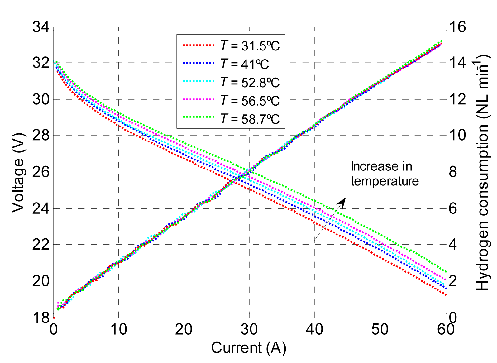
The test programmed in the electronic load consisted in always maintaining the same 60 A peak-to-peak sine wave component for a 30 s period whilst varying the DC component. This made it possible to obtain I-V curves for the different FC operating temperatures. The test was performed for 10, 20, 30, 40 and 60 A currents, obtaining operating temperatures of 31.5, 41, 52.8, 56.5 and 58.7 °C respectively. The methodology implemented made it possible to obtain an FC characterisation that was more complete than the one provided by the manufacturer. In addition, during the tests, the hydrogen consumption was measured.
The results obtained can be seen in Figure 4, plotting the I-V curves and the consumption of hydrogen in relation to temperature. The I-V curves show a non-linear relationship for currents of less than 20 A, this is due to the predominance of the activation losses. However, for the current range from 20 to 50 A, there is a highly linear relationship, primarily due to the predominance of the ohmic losses and to the fact that the activation losses remain relatively constant.
The influence of the concentration losses can be clearly seen above 50 A, where the FC voltage trend changes slightly, decreasing with a greater slope. On the other hand, it can be seen that the increased temperature favours the FC electricity supply, due to the fact that, for the same current, the FC output voltage increases. This is basically due to the increased activity of the redox semi-reactions and to the decrease in ionic resistance, leading to a reduction in the activation, ohmic and concentration losses. In addition, Figure 4 shows the hydrogen consumption in relation to the FC current, for an operating temperature range from 31.5 to 58.7 °C. It can be seen that a current increase leads to a consumption increase. Likewise, the dependence of consumption on temperature is very slight and, therefore, is not taken into account in the model.
4.1.2. Process to Obtain the Electrical Model Parameters Associated with the Steady-State Mode
Firstly, the parameters related to the consumption of the peripherals were obtained (k0, k1, k2). The current generated by the FC stack (is) is the sum of the current delivered by the FC (iFC) and the current shunted to the peripherals (iper) such as the fan, control circuits and purge valve [Equation (18)]. In order to establish the ratio between the currents, a test was conducted based on the demand made by a DC current from the FC from 0 to 60 A. When the FC reached the steady-state, for each current mode, the iFC, is and iper were measured. Based on these experimental data, specifically with the relationship between iFC and iper Equation (18) was fitted in order to obtain parameters k0, k1 and k2 shown in Table 1.
Likewise, the hydrogen pressure (pH2) must be obtained in order to obtain the reversible voltage. For this purpose, the above-mentioned tests were used, in which the pH2 was obtained in relation to the iFC in a steady-state operating mode. Parameters p0 and p1 were obtained by fitting Equation (3) to the experimental data of pH2 in relation to the iFC. Table 1 shows the characteristic parameter values for the thermodynamic phenomena obtained in the fitting.
Then the remaining parameters for the model were determined, related to the steady-state operating mode. These include parameter Rohm corresponding to the ohmic phenomena [Equation (15)], parameters a and b corresponding to the activation phenomena [Equation (8)] and parameters m and n corresponding to the concentration phenomena [Equation (11)]. However, given the fact that the experimental data were taken during continuous operation, the FC electrical model corresponds to the following equation:
By substituting Equations (8), (11) and (15) with Equation (34) the following expression is obtained:
Equation (35) is based on the stack current (is). Given that the experimental current corresponds with that generated by the FC (iFC) it is necessary to obtain is. To do so, the following expression is used, obtained from Equation (18):
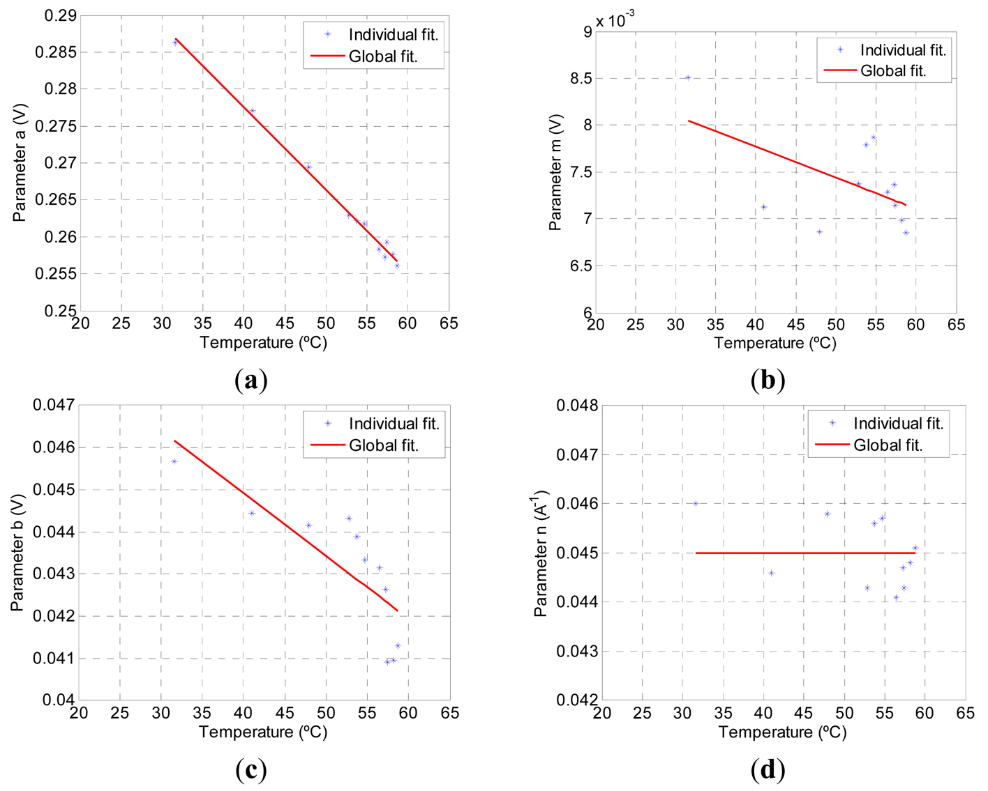
The process to obtain the parameters was made by fitting Equation (35) with the experimental I-V curves, similar to those plotted in Figure 4. When fitting Equation (35) to the experimental data, it is imposed that the value of parameter Rohm is that corresponding to the value obtained from the dynamic characterisation of the small signal detailed in Subsection 4.2.2. Once parameters Rohm, a, b, m and n have been obtained for each curve corresponding to an operating temperature, Equations (6), (7) and (12) are then fitted to these parameters. This gives coefficients a0, a1, b0, b1, m0 and m1 for these expressions, modelling the temperature influence on each parameter. The results of the individual experimental fitting of each parameter, based on temperature, in addition to the modelling of the parameters based on their expressions, are shown in Figure 5.
Where the parameters associated with the activation (a and b) can be seen to decrease as the temperature increases. This effect is associated with improved electrochemical reactions. In addition, parameter m also decreases with temperature, which implies that the concentration overvoltage decreases as the temperature increases. This effect is associated with the enhanced dissemination of the chemical species. The results of the coefficients obtained are shown in Table 1.
4.2. Electrochemical Impedance Spectroscopy
4.2.1. Characterisation of the Electrical Performance Associated with the Dynamic Mode
A frequency analysis was made in order to determine the experimental characterisation of the electrical performance of the FC in the dynamic operating mode, and to obtain the model parameters related thereto. The EIS technique applied to the FC consisted in drawing from the FC a DC current IDC with a small AC sine wave signal, δi, for a frequency spectrum. The EIS was conducted using the FRA and electronic load describe in Section 2.
The experimental tests conducted on the FC using the EIS technique, were based on drawing a DC current (IDC) of 5, 10 ,15, 20, 25, 30, 35, 40, 45, 50, 55 and 60 A corresponding to a temperature range from 20 to 62 °C. The current perturbation amplitude (δi) was 5% of IDC for a frequency range of 0.1 to 1000 Hz.
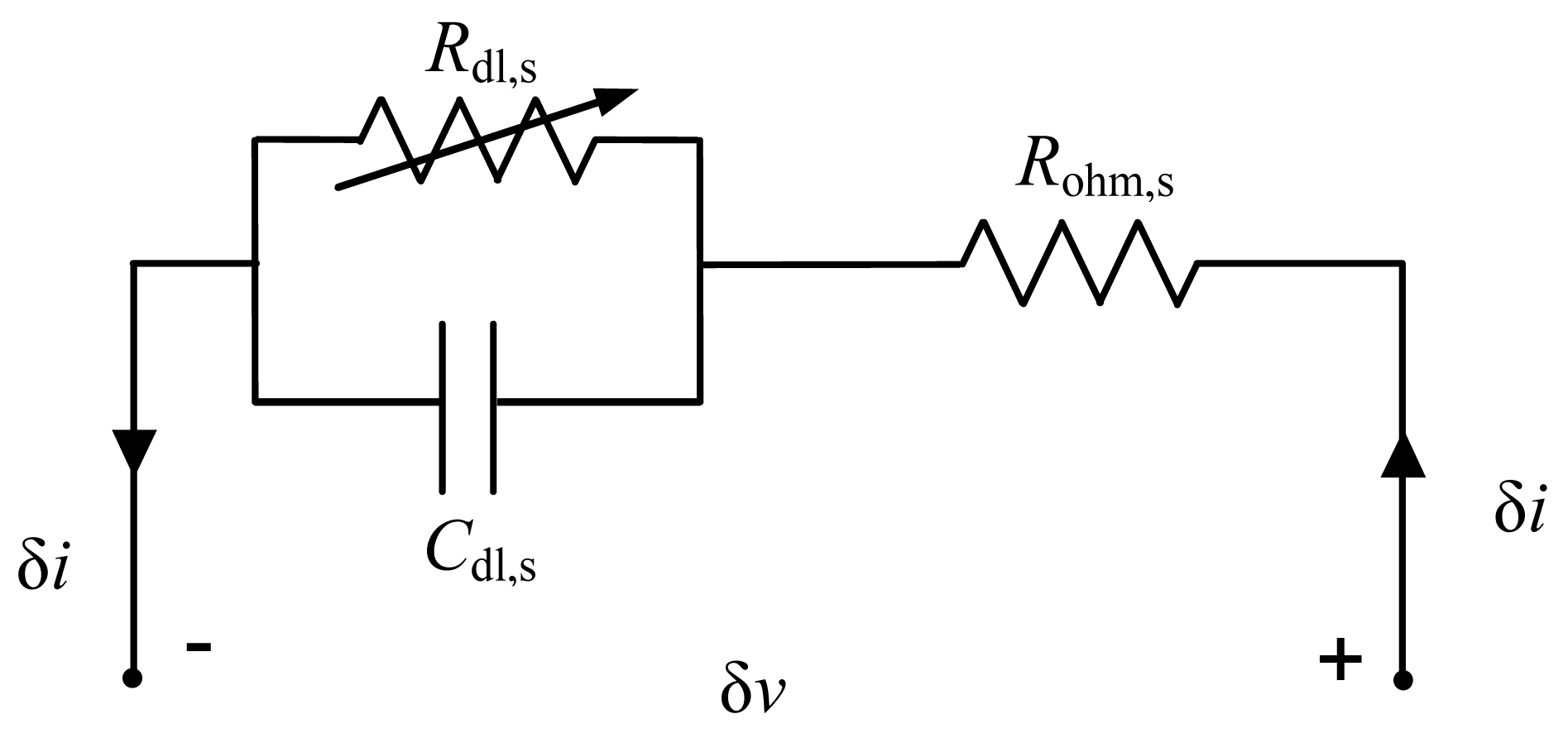
Following the EIS tests, the FC impedance was obtained, for the selected DC current point, from the small signal experimental amplitudes and phase shifts for voltage (δv) and current (δi) for each frequency. Figure 6 shows the electrical small signal equivalent circuit model, represented in Figure 2. This circuit is a small signal model of the FC performance and must therefore be fitted to the impedance values obtained in the frequency range used. Therefore, once the complete impedance of the FC was experimentally obtained for the frequency spectrum considered, the small signal circuit parameters were obtained for the various DC current stable points IDC, used for the tests.
Being small signal, the circuit shown in Figure 6 excludes the FC thermodynamic phenomena, in other words, Vrev,s. Likewise, given the fact that the experimental tests are based on small signal perturbations, the influence of the activation phenomena and concentration phenomena were modelled using resistors. The performance of the activation resistor and the concentration resistor were considered to be linear for each IDC of the impedance spectroscopy. In short, the current source and voltage source for the model in Figure 2 were replaced by double layer resistor Rdl,s, which is equal to the sum of the activation and concentration resistors. Therefore, this resistor represents the linearization of the activation and concentration phenomena, and can be calculated from the partial differentials of the activation and concentration voltages in relation to the current, and taking into account that iact,s and icon,s must be equal to the current at the point at which the small signal analysis is being made, that is, IDC.
4.2.2. Process to obtain the Electrical Model Parameters Associated with the Dynamic Mode
The determination of the parameters for the electrical model, associated with the dynamic mode, is based on the experimental results obtained in the EIS, with the impedance of the circuit shown in Figure 6. The equation for the impedance of the electrical circuit shown in Figure 6 is as follows:
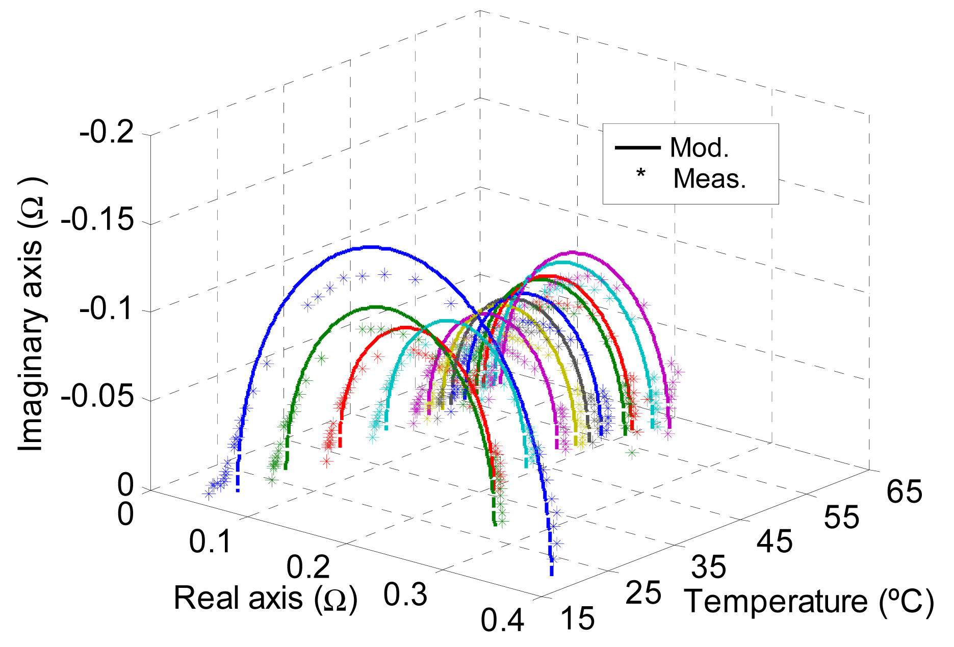
Figure 7 shows the experimental results obtained with the EIS applied to the FC, in addition to the modelling based on the small signal circuit shown in Figure 6, using Equation (37) with the parameter obtained in the fit. Each of the EIS tests, that is each Nyquist diagram corresponds to demanding a current from the FC. The said current imposes a temperature that is maintained constant during each test. Each asterisk corresponds to an impedance, with its real and imaginary part, obtained for a given frequency. Therefore, each EIS has its own specific temperature and current values. Observing, for each Nyquist diagram, the upward trend of the frequency data, it is possible to identify a semi-circle corresponding to the RC network for the small signal model. On the other hand, Figure 7 also shows that, as the temperature increases, the circumference area decreases until it reaches a temperature at which it starts to increase. This is due to the fact that, initially, more weighting is given to the reduction of the activation, concentration and ohmic losses which decrease with temperature. However, the test corresponding to high temperatures are conducted at a higher current, where the concentration phenomena start to carry considerably more weight.
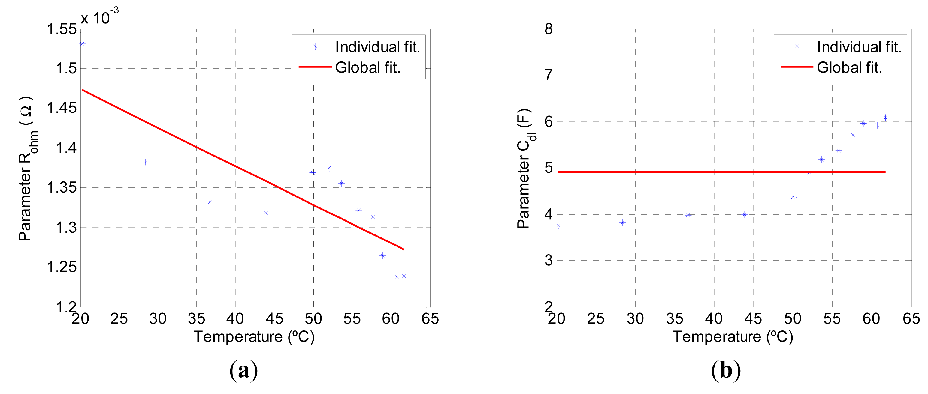
The parameters Rohm,s and Cdl,s were obtained by fitting the Equation (37), based on the experimental data shown in Figure 7, with the Toolbox Curve fitting by Matlab, for each temperature. These FC parameters are used to obtain Rohm and Cdl taking Ns into account, in other words through Equations (16) and (13) respectively. Once the Rohm parameters were obtained for each operating temperature, the fit was made using Equation (17). In this way, coefficients Rohm,0 and Rohm,1 were obtained, modelling the influence of temperature on each parameter. The individual result and the fit, based on the temperature of the said parameters, is shown in Figure 8. Parameter Rohm could be seen to fall as the temperature increased. This is primarily due to the fact that the membrane conductivity increases with temperature. On the contrary, parameter Cdl increases slightly at high temperatures, however, in order to simplify the model, it is considered to be independent of temperature (Cdl = 4.9183 F). With regard to the ohmic resistance, for a temperature of 60 °C, this acquires a value of 0.0012 Ω (0.18 Ω·cm2), similar to those obtained in [45,46]. The values of the said coefficients are shown in Table 1.
The EIS applied to the FCs makes it possible to characterise the FC dynamic mode, and also principally serves to identify parameters Rohm and Cdl. These values are considered to be independent of the current. This consideration was validated by performing additional EIS tests at different currents, whilst maintaining the temperature constant. Similar values were obtained for both parameters.
4.3. Thermal Performance
4.3.1. Characterisation and Process to Obtain the Parameters for the Thermal Model
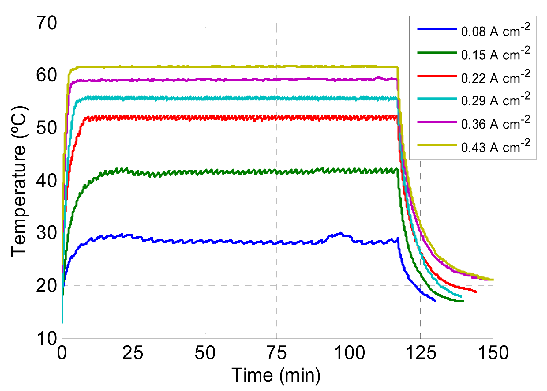
The thermal characterisation of the FC is performed through an analysis of the FC operating temperature evolution compared to the current drawn from the FC. For this purpose, a test was conducted during which a DC current was drawn from the FC with values of 10, 20, 30, 40, 50 and 60 A. Figure 9 shows the FC operating temperature evolution for the different current values. During these tests, the temperature was maintained at around 18 °C. It was observed that, the greater the current drawn from the FC, the lower the time taken to reach the stable operating temperature.
The parameters for the thermal model represented in Figure 3 were then obtained. In order to obtain the heating power for the sensible and latent heat, Equation (25) was used. For this purpose, the hydrogen consumption must be known. Based on the experimental data shown in Figure 4, a linear fit was made of the hydrogen consumption in relation to the current (Equation (28)). Parameter kf is shown in Table 2.
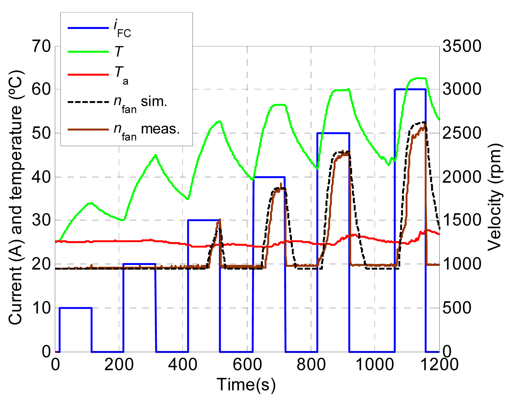
As was seen in Subsection 3.2, when determining the heat dissipated from the system, it is essential to know the air speed and, in turn, the air speed is dependent on the fan speed. In order to determine the fan speed, the test shown in Figure 10 was conducted, where currents of 10 to 60 A were drawn from the FC. The fan speed was shown to remain practically constant up to a T of 49 °C. Once this temperature had been reached, termed the reference temperature (Tref), the fan speed increased in proportion to the difference between T and Tref. This figure also shows the fit made for Equation (32) based on these experimental data. Likewise, it was observed that the minimum and maximum fan speeds were 945 rpm and 3100 rpm, respectively. Table 2 shows the parameters for nfan obtained for the fit of Equation (32).
Finally, the heat transfer coefficient (Ht) was obtained, which determines the dissipated heating power [Equation (31)]. The variable heat resistance (Rt) of the thermal model represented in Figure 3 was determined by the Ht inverse. The Ht primarily depends on the air speed and, consequently, on the fan speed. For this purpose, Ht was determined by means of an empirical expression, depending on the fan speed:
In order to obtain Ht the tests shown in Figure 9 were used. The experimental data for Ht, in addition to the fitting of the same by means of Equation (38) are shown in Figure 11. The parameters of this equation are shown in Table 2. This figure shows that as nfan increases, so does Ht. The values obtained for Ht are similar to those presented in Ref. [45].
5. Validation of the Modelling
5.1. Long-Duration Test
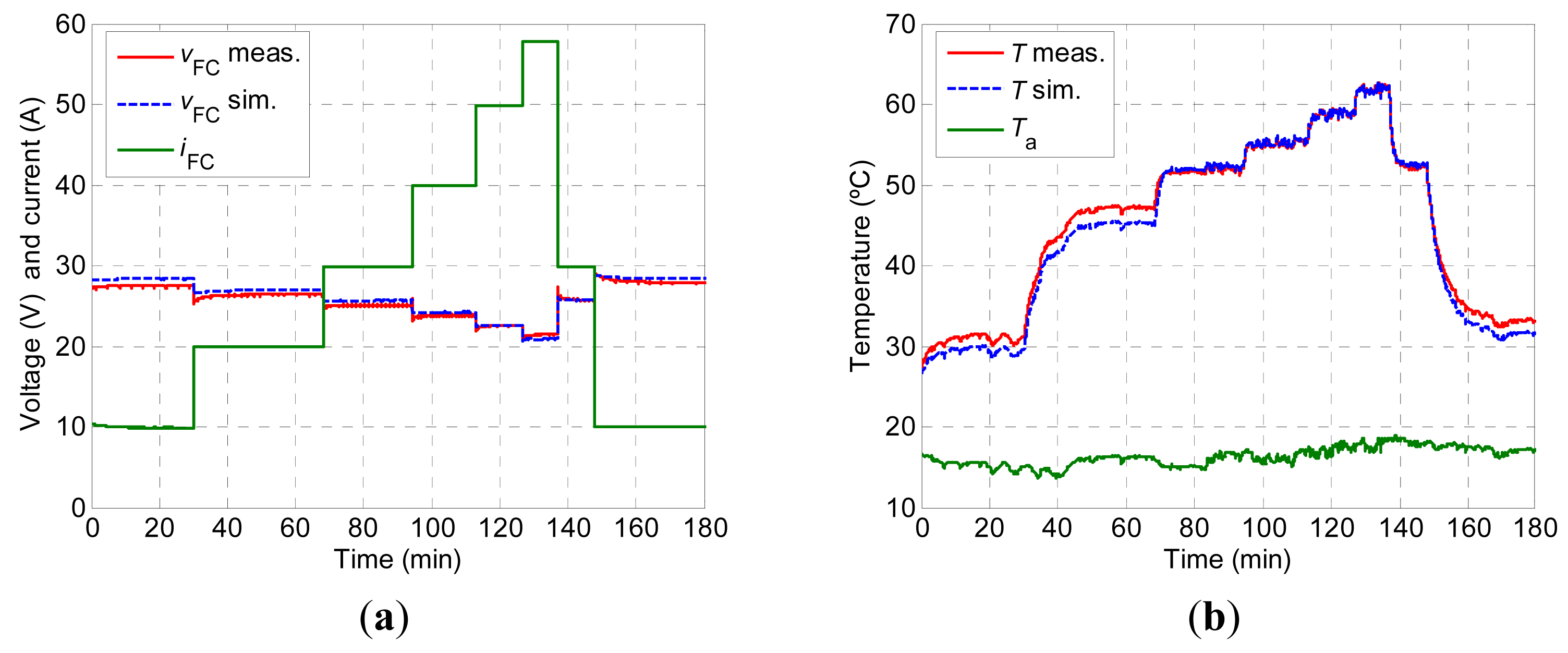
The long-duration validation of the models proposed was conducted by means of the test shown in Figure 12. In this test, a stepped current was drawn from the FC, from 10 to 58 A, with a 180 min duration, as shown in Figure 12a. It can be seen that, as the current drawn from the FC increases (iFC), the FC voltage decreases (vFC) and the FC operating temperature increases (T). It can be seen that the simulated vFC precisely follows the experimental vFC. It can be observed that, initially, the simulated vFC is slightly higher than the vFC measured, until the current drawn reaches 40 A, when both voltages are superimposed. On the other hand, for currents of more than 50 A, the simulated vFC is less than the measured vFC. Likewise, it can be observed that the largest deviation between both voltage values is at the time instant equal to 20 minutes, corresponding to a current step of 10 A. At this instant, the difference between both voltages is 0.86 V, corresponding to a relative error of 3.13%. Figure 12b shows the measured T, simulated T and ambient temperature (Ta) for the test corresponding to Figure 12a. It can be seen that the simulated T follows the trend of the measured T. In the second current step, where iFC is 20 A, the simulated T is less than the measured T. This interval shows the greatest deviation between both temperatures, with a difference of more than 2 °C. From then onwards, the simulated T follows the measured T more precisely. The modelling results obtained in the experiment shown in Figure 12 were quantified through the mean absolute percentage error (MAPE) and the root mean square error (RMSE). The results obtained are considered to be satisfactory, given the fact that, for the voltage, the MAPE is 2.01% and the RMSE 0.58 V and for the temperature the MAPE is 2.53% and the RMSE 1.21 °C. As can be seen, the voltage is predicted more accurately than the temperature. The deviations between the simulated temperature and the measured temperature may be due to the modelling of the fuel cell internal convection, due to the difficulty in characterising the fan speed.
5.2. Dynamic Test
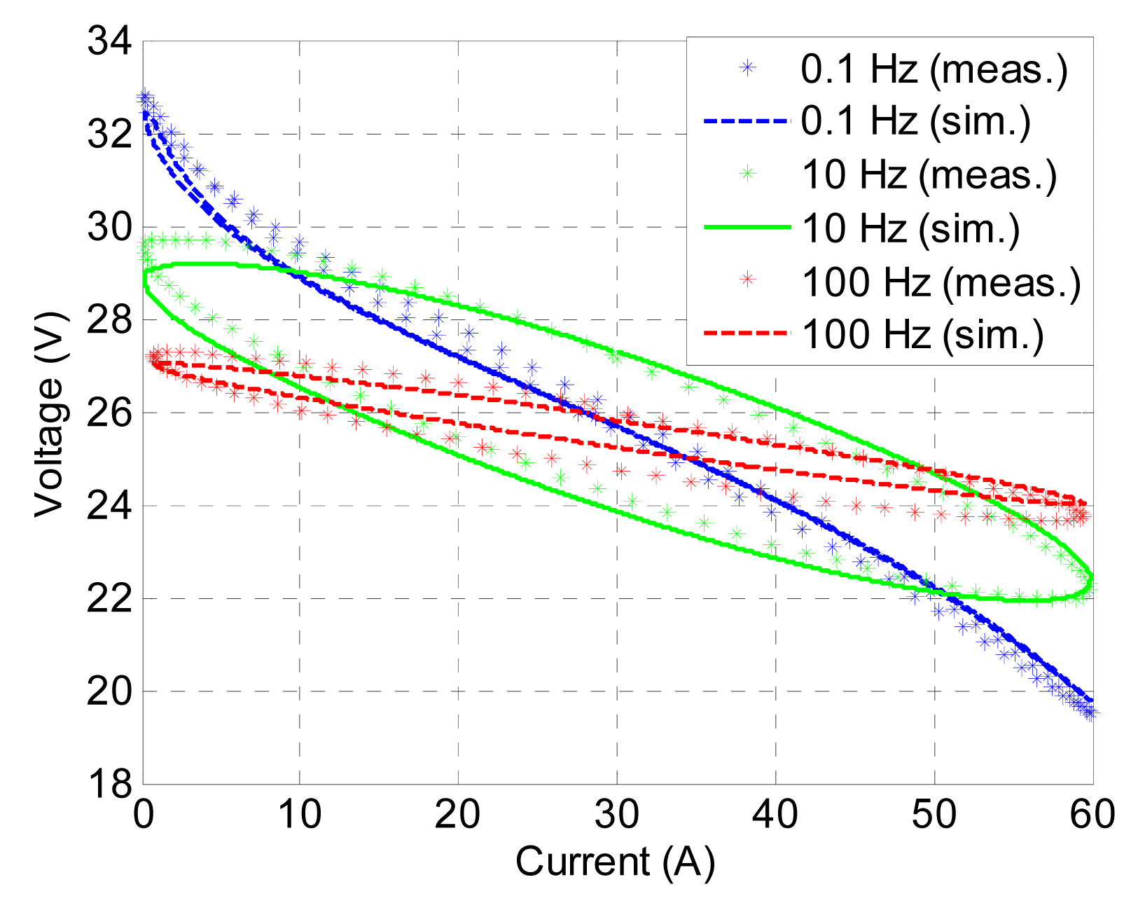
The dynamic validation of the models proposed was conducted through a test in which the FC was required to supply a sine wave current of various frequencies and with a peak-to-peak amplitude of 60 A, superimposed on a 30 A DC current. The test started with a frequency of 0.1 Hz and this was gradually increased to 100 Hz. Before conducting the dynamic tests, a current of 30 A was drawn from the FC for sufficient time to allow the operating temperature to stabilise at 52 °C and to remain constant throughout the dynamic test. Figure 13 shows the simulated and experimental current-voltage performance for frequencies of 0.1, 10 and 100 Hz.
It can be seen that, as the frequency increases (from 0.1 to 10 Hz), the area created in each current- voltage ratio starts to increase due to the fact that the double layer capacitance gradually absorbs the current and, therefore, the FC voltage and current gradually become out of phase. As the frequency increases (from 10 to 100 Hz), the current-voltage ratio gradually reduces its slope and starts to reduce its surface area. If the frequency were to be increased to high values, then the current-voltage area would disappear, as the double layer capacitance would be eliminated and the current-voltage relationship would be primarily determined by the FC ohmic resistance. Likewise, it can be observed that the FC model accurately reproduces the FC performance. A mean RMSE of 0.37 V and a mean MAPE of 1.25% was obtained, corresponding to the mean value of the RMSE and MAPE for the three tests.
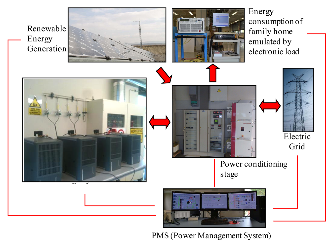
6. Analysis of the Operation of an FC System Integrated into a Microgrid
This section analyses the integration of an FC system into an electric microgrid located at the UPNa. Figure 14 shows a schematic diagram of the microgrid component parts. The microgrid renewable energy generating system comprises a PV generator and a wind turbine. The PV generator has a total power output of 4 kWp, whilst the rated power output of the wind turbine is 6 kW. The microgrid power conditioning system comprises a hybrid inverter incorporating the power conditioning stages for the microgrid devices. The storage system comprises four series-connected FCs, as described in Section 2, and modelled in Section 4, a hydrogen storage subsystem (described in Section 2) and there are also plans to install an electrolyser. The series-connected FCs have a total power output of 4800 W, a voltage range from 80 to 144 V and a maximum current of 60 A.
Furthermore, the microgrid has a management system (PMS) directed at the real time acquisition and control of the microgrid energy flows. In turn, the microgrid is equipped with a number of devices to monitor and measure the electrical and meteorological variables. The microgrid consumption is emulated through a programmable electronic load as described in Section 2. The electronic load emulation programming is based on real electricity consumption data, measured in a family home located close to the UPNa [10].
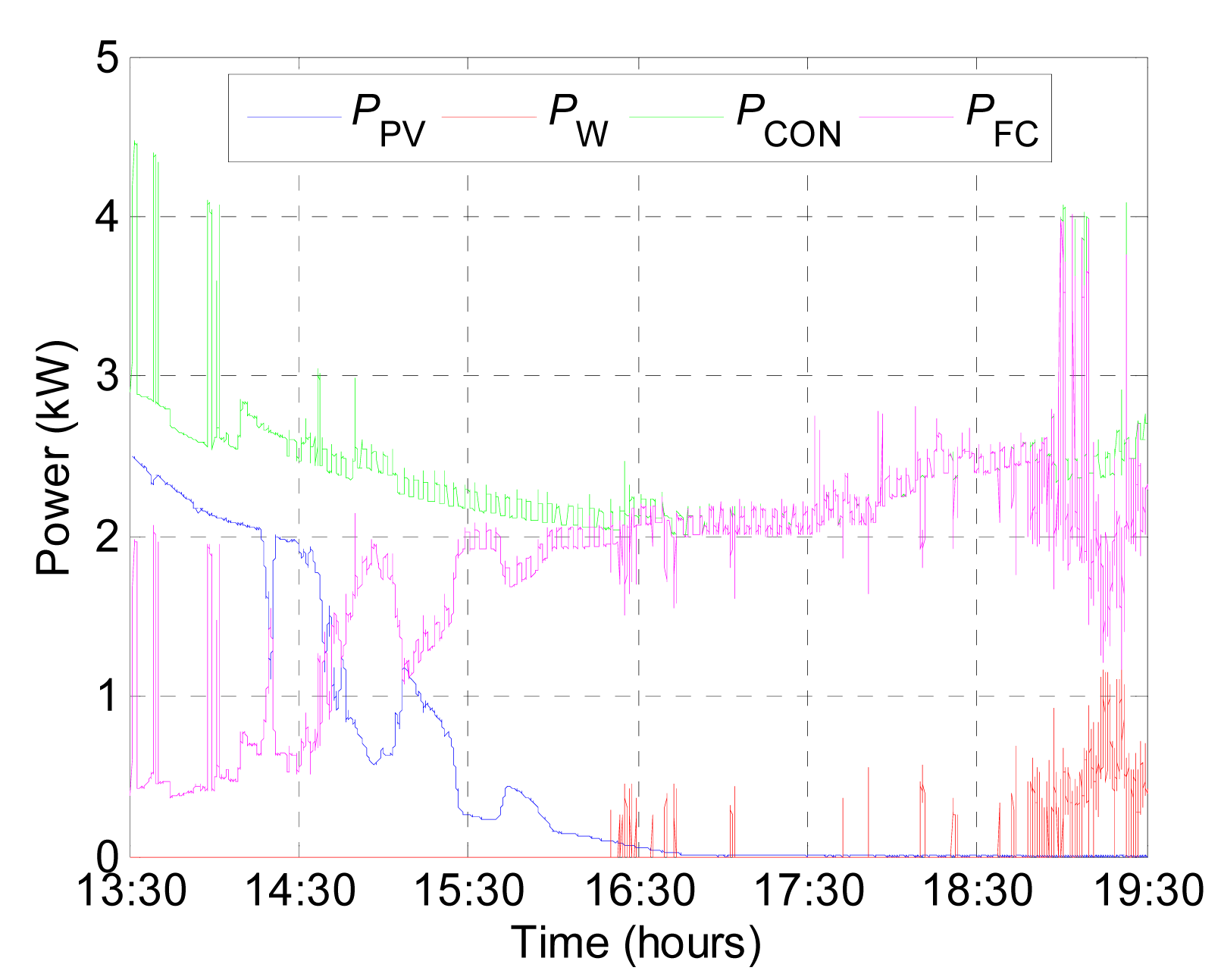
The analysis was made using a real power profile for the microgrid, with a duration of 6 hours. Figure 15 shows the PV power generated (PPV) and the wind power generated (PW) and the power consumed in the home (PCON) on the 9th December 2012 from 13:30 until 19:30 hours. This data was measured in the microgrid with a one second sampling time. PCON shows significant power variations due to the different loads connected throughout the period. Part of the consumption is practically constant and is primarily due to an electric heater, fridge and to the stand-by mode of a number of electric appliances such as the TV. Likewise, the day time consumption increased at lunch (13:30 h) and supper (19:00 h), primarily due to the connection of electric cooking appliances. PPV showed variations caused by the presence of scattered clouds. PW is low due to a low wind speed. The difference between the renewable power generated, in other words the sum of PW and PPV, and the power consumed is assumed by the storage system. In this analysis, the power of the storage system must be assumed by the four PEMFC (PFC) described in Section 2.
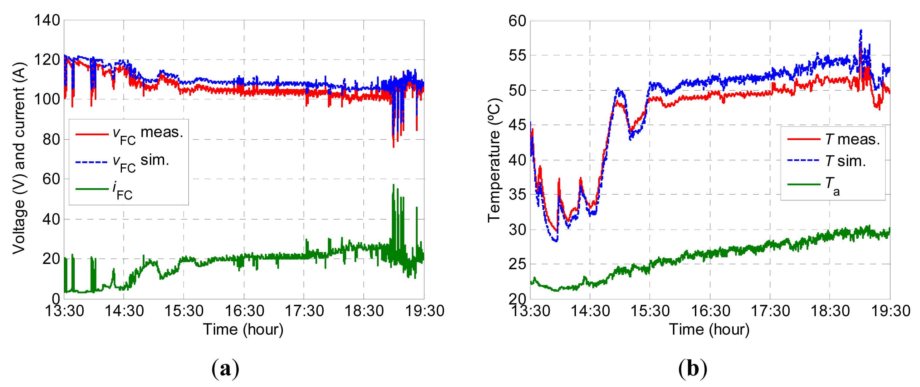
The DSP was used to program the microgrid storage system power profile of the microgrid into the electronic load. The FC system was subjected to the power profile of the microgrid storage system. Figure 16 shows the FC current and voltage corresponding to the power profile of the storage system (PFC) shown in Figure 16. It was observed that the current presented variations equivalent to the PFC, leading to considerable fluctuations in the FC voltage. At different time instants, the FC voltage dropped to values of less than 90 V. In addition, Figure 16a shows the simulated voltage for the model, which closely follows the experimental voltage. The simulated vFC is slightly higher than the experimental vFC. Specifically, the greatest deviation between both voltages is in the time interval from 15:30 to 18:30 h, where the iFC varies from14.6 to 30.58 A. For example, at the time instant equal to 15:30 h, where the iFC is 20.35 A, the experimental vFC reaches 104 V, whilst the simulated vFC is at 108 V. This deviation between both voltage values is equivalent to a relative error of less than 4%. On the contrary, for the time instant equal to 19:00 h, where iFC is 20.08 A, the experimental vFC reaches 109.5 V, whilst the simulated vFC is at 109.2 V. This deviation between both voltage values is equivalent to a relative error of less than 0.5%. Likewise, it can be observed that the simulated vFC offers similar dynamics to the experimental vFC. Figure 16b shows the experimental and simulated temperatures for the model, these temperatures are the mean operating temperature for each of the FCs. Likewise, the Ta is shown during the test, which gradually increases from 22 to 30 °C during the test. The T initially shows a downward trend and then subsequently rises. Moreover, it is shown to slightly decrease or increase whenever the current generated by the FCs decreases or increases. This same trend can be observed for the simulated temperature. As for the voltage, the simulated T is higher than the experimental one in the time interval from 15:30 to 19:00 hours. The results obtained are considered to be satisfactory, given the fact that a MAPE of 3.37% and a RMSE of 3.67 V was obtained for the voltage, and a MAPE of 4.17% and RMSE of 2.06 °C for the temperature. The increase in errors with regard to the other validations presented in Section 5 is basically due to the series connection of the four PEMFC. The four FC do not perform uniformly due to the manufacturing differences and because they do not have exactly the same operating hours, leading to a slight reduction in the accuracy of the models.
7. Conclusions
This article describes the modelling of a commercial 1.2 kW FC capable of predicting the FC voltage and operating temperature, based on the current demanded and the ambient temperature. The modelling was based on an electrical model and a thermal one. The electrical model proposed is based on the integration of the thermodynamic and activation, ohmic, concentration and double layer phenomena taking place in the FC, likewise the consumption of the peripherals was modelled. Whilst the thermal model proposed is based on the FC thermal energy balance, where the heat generation, dissipation mechanisms and FC thermal capacity were considered. An experimental characterisation was then performed for the electrical and thermal operation alike, making it possible to obtain the parameters for the FC models.
The models were implemented in Matlab Simulink in order to validate these models in a number of steady-state and dynamic operating environments. The validation results are considered to be satisfactory, given the fact that the simulations of the FC models accurately reproduce the electrical and thermal performance of the FCs. Specifically, a mean square error was obtained of less than 0.6 V for the FC voltage prediction, and a mean square error of less than 1.5 °C for the FC operating temperature prediction.
Likewise, the validation of the FC models was performed through the incorporation of four series-connected PEMFC with a rated power of 4.6 kW into a electric microgrid located at the Public University of Navarre. An analysis was made of the operation and the models were validated in a real microgrid operating environment. The results obtained demonstrate, on the one hand, that the FCs have adequate characteristics to adapt to requirements with regard to the power fluctuations caused by consumption and the microgrid generation. And, on the other hand, the model proposed accurately predicts the FC voltage and, therefore, can be used as a simulation tool to carry out the microgrid power output and energy management strategies.
Although, the FCs are able to assume the power fluctuations of the microgrid storage system profile, it may be advisable to incorporate a secondary storage system to provide a rapid response to variations of the PFC such as a bank of supercapacitors. In this way the FC would operate in less demanding conditions and, presumably, its useful life would be greater.
Acknowledgments
We acknowledge the Spanish Ministry of Economy and Competitiveness under grant DPI2010-21671-C02-01 and the Government of Navarre and FEDER funds under project “Microgrids in Navarra: design and implementation”.
Conflicts of Interest
The authors declare no conflict of interest.
References
- Lee, J.-Y.; Cha, K.-H.; Lim, T.-W.; Hur, T. Eco-efficiency of H2 and fuel cell buses. Int. J. Hydrog. Energy 2011, 36, 1754–1765. [Google Scholar]
- Hwang, J.J.; Chang, W.R. Life-cycle analysis of greenhouse gas emission and energy efficiency of hydrogen fuel cell scooters. Int. J. Hydrog. Energy 2010, 35, 11947–11956. [Google Scholar]
- Shaw, L.; Pratt, J.; Klebanoff, L.; Johnson, T.; Arienti, M.; Moreno, M. Analysis of H2 storage needs for early market “man-portable” fuel cell applications. Int. J. Hydrog. Energy 2013, 38, 2810–2823. [Google Scholar]
- Genconglu, M.T.; Zehra, U. Design of a PEM fuel cell system for residential application. Int. J. Hydrog. Energy 2009, 34, 5242–5248. [Google Scholar]
- Gray, E.M.; Webb, C.J.; Andrews, J.; Shabani, B.; Tsai, P.J.; Chan, S.L.I. Hydrogen storage for off-grid power supply. Int. J. Hydrog. Energy 2011, 36, 654–663. [Google Scholar]
- Ursúa, A.; Gandía, L.M.; Sanchis, P. Hydrogen production from water electrolysis: Current status and future trends. IEEE Proc. 2012, 100, 410–426. [Google Scholar]
- Leva, S.; Zaninelli, D. Hybrid renewable energy-fuel cell system: Design and performance evaluation. Electr. Power Syst. Res. 2009, 79, 316–324. [Google Scholar]
- Conte, M.; di Mario, F.; Iacobazzi, A.; Mattucci, A.; Moreno, A.; Ronchetti, M. Hydrogen as future energy carrier: The ENEA point of view on technology and application prospects. Energies 2009, 2, 150–179. [Google Scholar]
- Ursúa, A.; San Martín, I.; Barrios, E.L.; Sanchis, P. Stand-alone operation of an alkaline water electrolyser fed by wind and photovoltaic systems. Int. J. Hydrog. Energy 2013, 38, 14952–14967. [Google Scholar]
- San Martín, I.; Ursúa, A.; Sanchis, P. Integration of fuel cells and supercapacitors in electrical microgrids: Analysis, modelling and experimental validation. Int. J. Hydrog. Energy 2013, 38, 11655–11671. [Google Scholar]
- Obara, S. Analysis of a fuel cell micro-grid with a small-scale wind turbine generator. Int. J. Hydrog. Energy 2007, 32, 323–336. [Google Scholar]
- Zhou, T.; Francois, B. Modeling and control design of hydrogen production process for an active hydrogen/wind hybrid power system. Int. J. Hydrog. Energy 2009, 34, 21–30. [Google Scholar]
- Obara, S. Load response characteristics of a fuel cell micro-grid with control of number of units. Int. J. Hydrog. Energy 2006, 31, 1819–1830. [Google Scholar]
- San Martin, J.I.; Zamora, I.; San Martin, J.J.; Aperribay, V.; Eguia, P. Hybrid fuel cells technologies for electrical microgrids. Electr. Power Syst. Res. 2010, 80, 993–1005. [Google Scholar]
- O'Hayre, R.; Cha, S.; Colella, W.; Prinz, F.B. Fuel Cell Fundamentals; Wiley: Hoboken, NJ, USA, 2006. [Google Scholar]
- Larminie, J.; Dicks, A. Fuel Cell Systems Explained, 2nd ed.; Wiley: Hoboken, NJ, USA, 2003. [Google Scholar]
- Wang, Y.; Chen, K.S.; Mishler, J.; Cho, S.C.; Adroher, X.C. A review of polymer electrolyte membrane fuel cells: Technology, applications, and needs on fundamental research. Appl. Energy 2011, 88, 981–1007. [Google Scholar]
- Shah, A.A.; Luo, K.H.; Ralph, T.R.; Walsh, F.C. Recent and developments in polymer electrolyte membrane fuel cell modeling. Electrochim. Acta 2011, 56, 3731–3757. [Google Scholar]
- Biyikoglu, A. Review of proton exchange membrane fuel cell models. Int. J. Hydrog. Energy 2005, 30, 1181–1212. [Google Scholar]
- Cheddie, D.; Munroe, N. Review and comparison of approaches to proton exchange membrane fuel cell modeling. J. Power Sources 2005, 147, 72–84. [Google Scholar]
- Amphlett, J.C.; Baumert, R.M.; Mann, R.F.; Peppley, B.A.; Roberge, P.R. Performance modeling of the ballard IV solid polymer electrolyte fuel cell. Mechanistic model development. J. Electrochem. Soc. 1995, 142, 1–7. [Google Scholar]
- Amphlett, J.C.; Baumert, R.M.; Mann, R.F.; Peppley, B.A.; Roberge, P.R. Performance modeling of the ballard IV solid polymer electrolyte fuel cell. II. Empirical model development. J. Electrochem. Soc. 1995, 142, 9–15. [Google Scholar]
- Springer, T.; Zarwodzinski, T.; Gottesfeld, S. Polymer electrolyte fuel cell model. J. Electrochem. Soc. 1991, 138, 2334–2342. [Google Scholar]
- Kim, J.; Lee, S.M.; Srinivasan, S.; Chamberlin, C.E. Modeling of proton exchange membrane fuel cell performance with an empirical equation. J. Electrochem. Soc. 1995, 142, 2670–2674. [Google Scholar]
- Laurencelle, F.; Chahine, R.; Hamelin, J.; Agbossou, K.; Fournier, M.; Bose, T.K.; Laperrièrre, A. Characterization of a ballard MK5-E proton exchange membrane fuel cell stack. Fuel Cells 2001, 1, 66–71. [Google Scholar]
- Mann, R.F.; Amphlett, J.C.; Hooper, M.A.; Jensen, H.M.; Peppley, B.A.; Roberge, P.R. Development and application of a generalised steady-state electrochemical model for a PEM fuel cell. J. Power Sources 2000, 86, 173–180. [Google Scholar]
- Adzakpa, K.P.; Agbossou, K.; Dubé, Y.; Dostie, M.; Fournier, M.; Poulin, A. PEM fuel cells modeling and analysis through current and voltaje transient behaviors. IEEE Trans. Energy Convers. 2008, 23, 581–591. [Google Scholar]
- Barbir, F. PEM Fuel Cells: Theory and Practice; Elsevier: Burlinton, NY, USA, 2005. [Google Scholar]
- Iftikhar, M.U.; Riu, D.; Druart, F.; Rosini, S.; Bultel, Y.; Retiére, N. Dynamic of proton exchange membrane fuel cell using non integer derivatives. J. Power Sources 2006, 160, 1170–1182. [Google Scholar]
- Dhirde, A.M.; Dale, N.V.; Salehfar, H.; Mann, M.D.; Han, T. Equivalent electric circuit modeling and performance analysis of a PEM fuel cell stack using impedance spectroscopy. IEEE Trans. Energy Convers. 2010, 25, 778–786. [Google Scholar]
- Friede, W.; Rael, S.; Davat, B. Mathematical model and characterization of the transient behavior of PEM fuel cell. IEEE Trans. Power Electron. 2004, 19, 1234–41. [Google Scholar]
- Forrai, A.; Funato, H.; Yanagia, Y.; Kato, Y. Fuel cell parameter estimation and diagnostic. IEEE Trans. Power Electron. 2005, 20, 668–675. [Google Scholar]
- Reggiani, U.; Sandroli, L.; Giuliattini Burbui, G.L. Modelling a PEM fuel cell stack with a nonlinear equivalent circuit. J. Power Sources 2007, 165, 224–231. [Google Scholar]
- Jung, J.H.; Ahmed, S.; Enjeti, P. PEM fuel cell stack model development for real-time simulation applications. IEEE Trans. Ind. Electron. 2011, 58, 4217–4231. [Google Scholar]
- Fontes, G.; Turpin, C.; Astier, S.; Meynard, T.A. Interactions between fuel cells and power converters: Influence of current harmonics on a fuel cell stack. IEEE Trans. Power Electron. 2007, 22, 670–678. [Google Scholar]
- Niya, S.M.R.; Hoorfar, M. Study of proton exchange fuel cells using electrochemical impedance spectroscopy technique—A review. J. Power Sources 2013, 240, 281–293. [Google Scholar]
- Wingelaar, P.J.H.; Duarte, J.L.; Hendrix, M.A.M. PEM fuel cell model representing steady state, small signal and large signal characteristics. J. Power Sources 2007, 171, 754–762. [Google Scholar]
- Del Real, A.J.; Arce, A.; Bordons, C. Development and experimental validation of a PEM fuel cell dynamic model. J. Power Sources 2007, 173, 310–324. [Google Scholar]
- Latha, K.; Vidhya, S.; Umamaheswari, B.; Rajalakshmi, N.; Dhathathreyan, K.S. Tuning of PEM fuel cell model parameters for prediction of steady state and dynamic performance under various operating conditions. Int. J. Hydrog. Energy 2013, 38, 2370–2386. [Google Scholar]
- Ferrero, R.; Marracci, M.; Prioli, M.; Tellini, B. Simplified model for evaluating ripple effects on commercial PEM fuel cell. Int. J. Hydrog. Energy 2012, 37, 3462–3469. [Google Scholar]
- Amphlett, J.C.; Mann, R.F.; Roberge, P.R.; Rodrigues, A. A model predicting transient response of proton exchange membrane fuel cells. J. Power Sources 1996, 61, 183–188. [Google Scholar]
- Wang, C.; Nehrir, M.H.; Shaw, S.R. Dynamic models and model validation for PEM fuel cells using electrical circuits. IEEE Trans. Energy Convers. 2005, 20, 442–451. [Google Scholar]
- Khan, M.J.; Iqbal, M.T. Modelling and analysis of electrochemical, thermal, and reactant flow dynamics for a PEM fuel cell system. Fuel Cells 2005, 4, 463–475. [Google Scholar]
- Musio, F.; Tacchi, F.; Omati, L.; Stampino, P.G.; Dotelli, G.; Limonta, S.; Brivio, D.; Grassini, P. PEMFC system simulation in MATLAB-Simulink environment. Int. J. Hydrog. Energy 2011, 36, 8045–8052. [Google Scholar]
- Kim, H.; Cho, C.Y.; Nam, J.; Shim, D.; Chung, T.Y. A simple dynamic model for polymer electrolyte membrane fuel cell (PEMFC) power modules: Parameter estimation and model prediction. Int. J. Hydrog. Energy 2010, 35, 3656–3663. [Google Scholar]
- Ramos-Paja, C. A.; Giral, R.; Martinez-Salamero, L.; Romano, J; Romero, A.; Spagnuolo, G.A. PEM fuel-cell model featuring oxygen-excess-ratio estimation and power-electronics interaction. IEEE Trans. Ind. Electron. 2010, 57, 1914–1924. [Google Scholar]
- Tiss, F.; Chouikh, R.; Guizani, A. Dynamic modeling of a PEM fuel cell with temperature effects. Int. J. Hydrog. Energy 2012, 38, 8532–8541. [Google Scholar]
- Gao, F.; Blunier, B.; Miraoui, A.; El-Moudni, A. Cell layer level generalized dynamic modeling of a PEMFC stack using VHDL-AMS language. Int. J. Hydrog. Energy 2009, 34, 5498–521. [Google Scholar]
- Gao, F.; Blunier, B.; Miraoui, A.; El-Moudni, A. Proton exchange membrane fuel cell multi-physical dynamics and stack spatial non-homogeneity analyses. J. Power Sources 2010, 195, 7609–7626. [Google Scholar]
- Hou, Y.; Shen, C.; Yang, Z.; He, Y. A dynamic voltage model of a fuel cell stack considering the effects of hydrogen purge operation. Renew. Energy 2012, 44, 246–251. [Google Scholar]
- Men, H. Y. Numerical studies of liquid water behaviors in PEM fuel cell cathode considering transport across different porous layers. Int. J. Hydrog. Energy 2010, 35, 5569–5579. [Google Scholar]
- Alink, R.; Gerteisen, D. Modeling the liquid water transport in the gas diffusion layer for polymer electrolyte membrane fuel cells using a water path network. Energies 2013, 6, 4508–4530. [Google Scholar]
- Quan, P.; Lai, M.C. Numerical study of water management in the air flow channel of a PEM fuel cell cathode. J. Power Sources 2007, 164, 222–237. [Google Scholar]
- Baschuk, J.J.; Xianguo, L. Modeling of ion and water transport in the polymer electrolyte membrane of PEM fuel cells. Int. J. Hydrog. Energy 2010, 35, 5095–5103. [Google Scholar]
- Obayopo, S.O.; Bello-Ochende, T.; Meyer, J.P. Modelling and optimization of reactant gas transport in a PEM fuel cell with a transverse pin fin insert in channel flow. Int. J. Hydrog. Energy 2012, 37, 10286–10298. [Google Scholar]
- Gerteisen, D.; Hakejos, A.; Schumacher, J.O. AC impedance modelling study on porous electrodes of proton exchange membrane fuel cells using agglomerate model. J. Power Sources 2007, 173, 346–356. [Google Scholar]
- Hwang, J.J. A complete two-phase model of a porous cathode of a PEM fuel cell. J. Power Sources 2007, 164, 174–181. [Google Scholar]
- Pharoaha, J.G.; Karana, K.; Suna, W. On effective transport coefficients in PEM fuel cell electrodes: Anisotropy of the porous transport layers. J. Power Sources 2006, 161, 214–224. [Google Scholar]
- Wang, Y.; Wang, C.Y. Transient analysis of polymer electrolyte fuel cells. Electrochim. Acta 2005, 50, 1307–1315. [Google Scholar]
- Wang, Y.; Wang, C.Y. Dynamics of polymer electrolyte fuel cells undergoing load changes. Electrochim. Acta 2006, 52, 3924–3933. [Google Scholar]
- Çengel, Y.A. Transferencia de Calor; Mc Graw Hill: Mexico, Mexico, 2004. [Google Scholar]
- Shahsavari, S.; Desouza, A.; Bahrami, M.; Kjeang, E. Thermal analysis of air-cooled PEM fuel cells. Int. J. Hydrog. Energy 2012, 37, 18261–18271. [Google Scholar]
Nomenclature
| Symbols | |
|---|---|
| A | Area (cm2) |
| a,b | Parameters associated with activation phenomena |
| ai, bi | Coefficients associated with activation phenomena |
| Cdl | Double layer capacitance (F) |
| cp | Specific heat (J g−1 °C−1) |
| Cth | Thermal capacity (J °C−1) |
| F | Faraday constant (96485 C mol−1) |
| fH2 | Hydrogen consumption (NL min−1) |
| Ht | Heat transfer coefficient (J s−1 °C−1) |
| Hv | Enthalpy of vaporization (J g−1) |
| i | Current (A) |
| i0 | Exchange current (A) |
| IDC | DC current (A) |
| kf | Parameter associated with hydrogen consumption |
| kfan | Parameter associated with fan velocity |
| ki | Parameters associated with peripherals |
| m | Mass (g) |
| m, n | Parameters associated with concentration phenomena |
| mi | Coefficients associated with concentration phenomena |
| ṁ | Mass flow rate (g s−1) |
| M | Molar mass (g mol−1) |
| Ns | Number of series cells |
| nfan | Fan velocity (rpm) |
| nfan,min | Minimum fan velocity (rpm) |
| P | Power (W) |
| p | Pressure (bar) |
| p0, p1 | Parameters associated with the hydrogen pressure |
| Q̇ | Heat flow rate (W) |
| R | Resistance (Ω) |
| Rg | Ideal gas constant (8.314 J mol−1 K−1) |
| Rohm | Parameters associated with ohmic phenomena |
| Rohm,i | Coefficients associated to ohmic phenomena |
| T | Temperature (°C) |
| v | Voltage (V) |
| Vrev | Reversible voltage (V) |
| Z | Impedance (Ω) |
| z | Number of electrons transferred in the reaction |
| Δh0f | Enthalpy of formation (J mol−1) |
| α | Transfer coefficient |
| Abbreviations | |
|---|---|
| AFC | Alkaline FC |
| DMFC | Direct methanol FC |
| DSP | Digital signal processor |
| MCFC | Molten carbonate FC |
| PAFC | Phosphoric acid FC |
| PEMFC | Proton exchange membrane FC |
| EIS | Electrochemical impedance spectroscopy |
| FC | Fuel cell |
| FRA | Frequency response analyzer |
| MAPE | Mean absolute percentage error |
| PMS | Power Management System |
| RMSE | Root mean square error |
| SOFC | Solid oxides FC |
| UPNa | Public University of Navarre |
| Subscripts | |
|---|---|
| a | Ambient |
| act | Activation |
| c | Chemical |
| con | Concentration |
| CON | Consumption |
| dl | Double layer |
| e | Evacuated |
| FC | Fuel cell |
| g | Generated |
| H2 | Hydrogen |
| H2O | Water |
| l | Liquid |
| la | Latent |
| n | Net |
| O2 | Oxygen |
| ohm | Ohmic |
| per | Peripheral |
| PV | Photovoltaic |
| ref | Reference |
| s | Stack |
| se | Sensible |
| v | Vapour |
| W | Wind |


| Description | Parameter | Value |
|---|---|---|
| Peripheral consumption | k0(A) | 1.5240 |
| k1 | −1.2080 × 10⁻³ | |
| k2 (A−1) | 4.1180 × 10⁻⁴ | |
| Thermodynamic phenomenon | P0 (bar) | 1.3240 |
| P1 (bar·A−1) | −1.3050 × 10⁻⁴ | |
| Activation phenomenon | a0 (V) | 0.6259 |
| a1 (V·°C−1) | −1.1128 × 10⁻³ | |
| b0 (V) | 9.1487 × 10⁻² | |
| b1 (V·°C−1) | −1.4866 × 10⁻⁴ | |
| Concentration phenomenon | m0 (V) | 1.8250 × 10⁻² |
| m1 (V·°C−1) | −3.3280 × 10⁻⁵ | |
| n (A−1) | 4.500 × 10⁻² | |
| Ohmic phenomenon | Rohm,0 (Ω) | 2.8959 × 10⁻³ |
| Rohm,1 (Ω·°C−1) | −4.8479 × 10⁻⁶ | |
| Double layer phenomenon | Cdl (F) | 4.9183 |
| Description | Parameter | Value |
|---|---|---|
| Hydrogen consumption | kf (NL·min−1·A−1) | 0.2547 |
| Fan velocity | nfan,min (rpm) | 945 |
| kfan (rpm·°C−1) | 122.9 | |
| Tref (°C) | 49 | |
| Heat transfer coefficient | kHt,1 (W·°C−1·rpm−1) | 0.0136 |
| kHt,2 (W·°C−1) | 0.6600 | |
© 2014 by the authors; licensee MDPI, Basel, Switzerland This article is an open access article distributed under the terms and conditions of the Creative Commons Attribution license ( http://creativecommons.org/licenses/by/3.0/).
Share and Cite
San Martín, I.; Ursúa, A.; Sanchis, P. Modelling of PEM Fuel Cell Performance: Steady-State and Dynamic Experimental Validation. Energies 2014, 7, 670-700. https://doi.org/10.3390/en7020670
San Martín I, Ursúa A, Sanchis P. Modelling of PEM Fuel Cell Performance: Steady-State and Dynamic Experimental Validation. Energies. 2014; 7(2):670-700. https://doi.org/10.3390/en7020670
Chicago/Turabian StyleSan Martín, Idoia, Alfredo Ursúa, and Pablo Sanchis. 2014. "Modelling of PEM Fuel Cell Performance: Steady-State and Dynamic Experimental Validation" Energies 7, no. 2: 670-700. https://doi.org/10.3390/en7020670