Convex Optimization for the Energy Management of Hybrid Electric Vehicles Considering Engine Start and Gearshift Costs

Abstract

This paper presents a novel method to solve the energy management problem for hybrid electric vehicles (HEVs) with engine start and gearshift costs. The method is based on a combination of deterministic dynamic programming (DP) and convex optimization. As demonstrated in a case study, the method yields globally optimal results while returning the solution in much less time than the conventional DP method. In addition, the proposed method handles state constraints, which allows for the application to scenarios where the battery state of charge (SOC) reaches its boundaries.

1. Introduction

Hybrid electric vehicles (HEVs) are one option to reduce the CO₂ emissions of passenger light-duty vehicles. Such hybrid vehicles consist of at least two power sources, typically an internal combustion engine and one or more electric motors, as well as an energy buffer, typically a battery. The control of the power flows among these devices is commonly referred to as the energy management or supervisory control [1]. There are many approaches [2] to design an energy management strategy, covering heuristic approaches [3–6] as well as optimization-based approaches, such as deterministic dynamic programming (DP) [7–13], Pontryagin's minimum principle (PMP) [14–21] and stochastic dynamic programming (SDP) [22–26]. Recently, convex optimization [27] has attracted attention in the research field of energy management for HEVs. It is seen as an alternative method for the optimization of the power flows in HEVs with the advantage of being computationally more efficient than for example DP or indirect methods such as PMP are. Convex optimization has already been employed for dimensioning of powertrains [28–30], energy efficiency analysis [31] and online control of HEVs [32,33]. However, inherently discrete decision variables, such as the engine on/off decision or the gear decision, are typically determined using heuristic approximations. The reason is the fact that discrete signals are not convex and thus cannot be optimized using convex optimization. One approach to optimize discrete decision problems is to solve a mixed-integer problem [32], but its drawback is the large computational burden for optimizations on typical driving missions. A more efficient approach consists of splitting up the problem into two parts, where the discrete decision variables are optimized prior to the convex optimization [33] with the possibility to iterate between the two steps [34]. Based on this methodology, the authors of [30] showed that the optimal engine on/off strategy can be calculated for a serial HEV.

However, in all those convex optimization approaches, costs for switching the engine on/off state or changing the gears are not considered. As reported for instance in [35,36], applying optimization-based methods for the energy management of parallel hybrid vehicles without penalizing engine start or gearshift events can lead to unacceptably frequent engine starts and gearshifts, eventually leading to an increased fuel consumption, excessive wear of components and/or an uncomfortable driving experience. Therefore, in the DP, PMP and SDP approaches, researchers [26,37–41] have introduced penalties or costs for the changes in the engine or the gear state such that unacceptably frequent starts and shifts can be prevented. To do so in convex optimization-based approaches, heuristics based on signal filtering have been presented so far [29]. However, a corresponding optimal solution for methods relying on convex optimization has yet to be found.

Therefore, this paper presents a method to solve the energy management problem for a parallel HEV taking such engine start and gearshift costs into account by using a combination of convex optimization and DP. In a case study, the method is shown to converge to the globally optimal solution while still being computationally efficient. Moreover, the proposed method can handle state constraints. Although not presented in this paper, the algorithm can potentially be applied to an efficient sizing of hybrid powertrains or to the on-board control of hybrid vehicles in the form of receding horizon control.

The paper is structured as follows: Section 2 details the vehicle model used,; Section 3 explains the mathematical problem; Section 4 presents the novel method; Section 5 compares the novel method to DP; Section 6 discusses the novel method; and Section 7 concludes on the ideas shown in this paper.

2. Vehicle Model

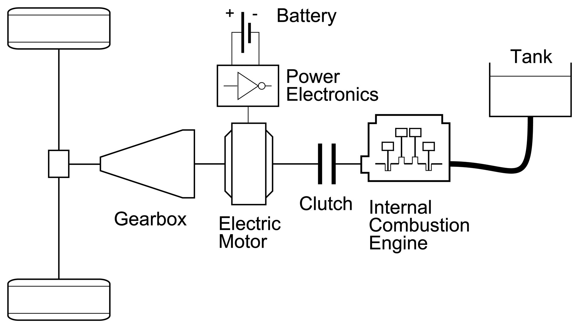
The vehicle under investigation is a pre-transmission parallel HEV passenger car of the executive class. Figure 1 illustrates the configuration of the powertrain architecture which consists of an automatic gearbox, an electric motor, the power electronics, a battery, a clutch and a turbocharged spark-ignited internal combustion engine. The vehicle does not exist yet physically, therefore, the basis for the subsequent vehicle model is a generic vehicle model according to commonly accepted modeling standards [1]. To simulate the vehicle, a quasi-static backward approach is used. This widely adopted method of simulation [8,12,42,43] was shown to yield reasonable estimates of fuel consumption when compared to measurement data [44].

2.1. Introduction to Convex Vehicle Modeling

In order to apply the concepts presented in Section 4 below, the generic, nonlinear vehicle model has to be approximated by a convex model, see [27] for a general introduction to convex optimization, and [29,45] for an introduction to convex modeling and optimization of HEVs.

A convex description of the model requires the component models to be expressed as a convex function of the free optimization variables which are used by the convex solver. These free optimization variables typically comprise more free variables than are actually required to solve the problem using different methods such as, for instance, DP. Examples of such free optimization variables are the torques of the motor and the engine, the electrical power consumption of the motor, the fuel consumption, the battery current and the battery state of charge (SOC). Inherently discrete variables, such as the engine on/off decision or the gear decision, are not convex, and thus, they cannot be included in a convex description. However, for given trajectories of the non-convex variables, the remaining model can be convex.

In this paper, the energy management of the vehicle is assumed to have three decision variables, namely the engine on/off, the gear, and the torque split between the engine and the motor. Since the engine on/off and the gear decision are inherently discrete, these variables are assumed to be known prior to solving a convex optimization problem. The only convex decision variable is the torque split. Therefore, the power flows from the road load up to the gearbox input, where the torque split is decided, can be expressed by any nonlinear function. Only the power flows upstream of the gearbox input have to be described in a convex form. In the following, the approximations needed to obtain a suitable model are explained in detail. All vehicle parameters used in the model are listed in

Table 1. Parameters of the pre-transmission parallel HEV executive class passenger car. SOC: state of charge.

Parameter	Symbol	Value
Wheel radius	rw	0.32 m
Air density	ρair	1.24 kg/m3
Effective frontal area	cd · A	0.60 m2
Rolling friction coef.	cr	0.012
Gravit. constant	ag	9.81 m/s2
Total vehicle mass	mυ	1800 kg
Rot. equiv. mass (gear-dep.)	mr	[129, 84, 72, 61, 55, 52, 51] kg
Gear ratios	ig	[10.8, 7.1, 4.7, 3.4, 2.5, 2.0, 1.8]
Gearbox efficiency param.	ηg,0	0.95
Gearbox efficiency param.	ηg,1	0.02 1/(rad/s)
Gearbox efficiency param.	ωg,1	400 rad/s
Nominal motor power		40 kW
Max. motor speed	ωm,max	628 rad/s
Nominal engine power		150 kW
Min. engine speed	ωe,min	105 rad/s
Max. engine speed	ωe,max	628 rad/s
Max. battery capacity	Q0	7.64 A h
Open circuit voltage	Voc	263 V
Battery int. resistance	Ri	0.24 Ω
Min. battery current	Ib,min	−200 A
Max. battery current	Ib,max	200 A
Min. SOC	SOCmin	0.20
Max. SOC	SOCmax	0.80
Aux. power demand	Paux	400 W

.

2.2. Road Load Model

Assuming that a quasi-static driving cycle is represented by its velocity υ, acceleration a, and road slope α for each instant in time k ∈ {1, 2, …, N}, the wheel speed ω_w and the wheel torque T_w required to follow the driving cycle are calculated by [1]:

$${\omega }_w(k)=\frac{\upsilon (k)}{r_w}$$

(1)

$$T_w(k)=r_w\cdot (\frac{1}{2}{\rho }_{\text{air}}{c}_{d}A{\upsilon }^2(k)+c_r{m}_{\upsilon }{a}_{g}cos(\alpha (k))+m_{\upsilon }{a}_{g}sin(\alpha (k))+(m_{\upsilon }+m_r(g(k)))a(k))$$

(2)

The variable r_w denotes the wheel radius, ρ_air the air density, c_d the aerodynamic drag coefficient, A the frontal area of the vehicle, c_r the rolling friction coefficient, m_υ the total vehicle weight, a_g the gravitational acceleration, m_r the equivalent mass of the rotating parts of the powertrain, and g the gear engaged (m_r depends on the choice of the gear).

2.3. Gearbox Model

The speed ω_g and the torque T_g at the gearbox input are calculated by:

$${\omega }_g(k)={\omega }_w(k)\cdot i_g(k)$$

(3)

$$T_g(k)=T_w(k)\cdot \frac{1}{i_g(k)}\cdot {({\eta }_{g,0}-\frac{{\eta }_{g,1}}{{\omega }_{g,1}}\cdot {\omega }_g(k))}^{-\text{sign}(T_w(k))}$$

(4)

with i_g being the gear ratio of gear g ∈ {1, …, 7}, and η_g,0, η_g,1, ω_g,1 being the parameters to model the speed-dependent gearbox losses which account for the increased friction at higher gearbox input speeds [46]. The values for the efficiency parameters were chosen based on expert knowledge.

Moreover, losses occurring during gearshifts are assumed to consume m_g = 0.01 g fuel equivalent per gearshift, i.e.,

$$m_g(k)=\{\begin{array}{ll}0.01\text{g}\hfill & \text{if}g(k)\ne g(k-1)\hfill \\ 0\hfill & \text{else}\hfill \end{array}$$

(5)

The gear g is assumed to be controlled by the gear control variable u_g:

$$\begin{array}{ll}g(k)=g(k-1)+u_g(k),\hfill & u_g\in \{-1,0,1\}\hfill \end{array}$$

(6)

These shift losses in Equation (5) account for the fuel-equivalent energetic effort to change the gears. The losses can be estimated by first principle models similarly to those presented in [47,48] for a dual-clutch transmission. Otherwise, for the optimization, some artificial shift costs can be assigned in order reduce the number of gearshifts. These artificial shift costs are then considered in the cost function of the optimization without including them in the calculation of the fuel consumption [10,26,40]. For the method presented in this paper, the model for the gearshift costs is not restricted to the form presented in Equation (5). More complex models are allowed since the gear control variable is not optimized via convex optimization.

2.4. Torque Split Model

The torque split between the electric motor and the internal combustion engine is determined by the motor torque u_ts ≜ T_m such that the engine torque T_e is determined by:

$$T_e(k)=T_g(k)-u_{ts}(k)$$

(7)

This equation is convex in any of the variables involved.

2.5. Electric Motor Model

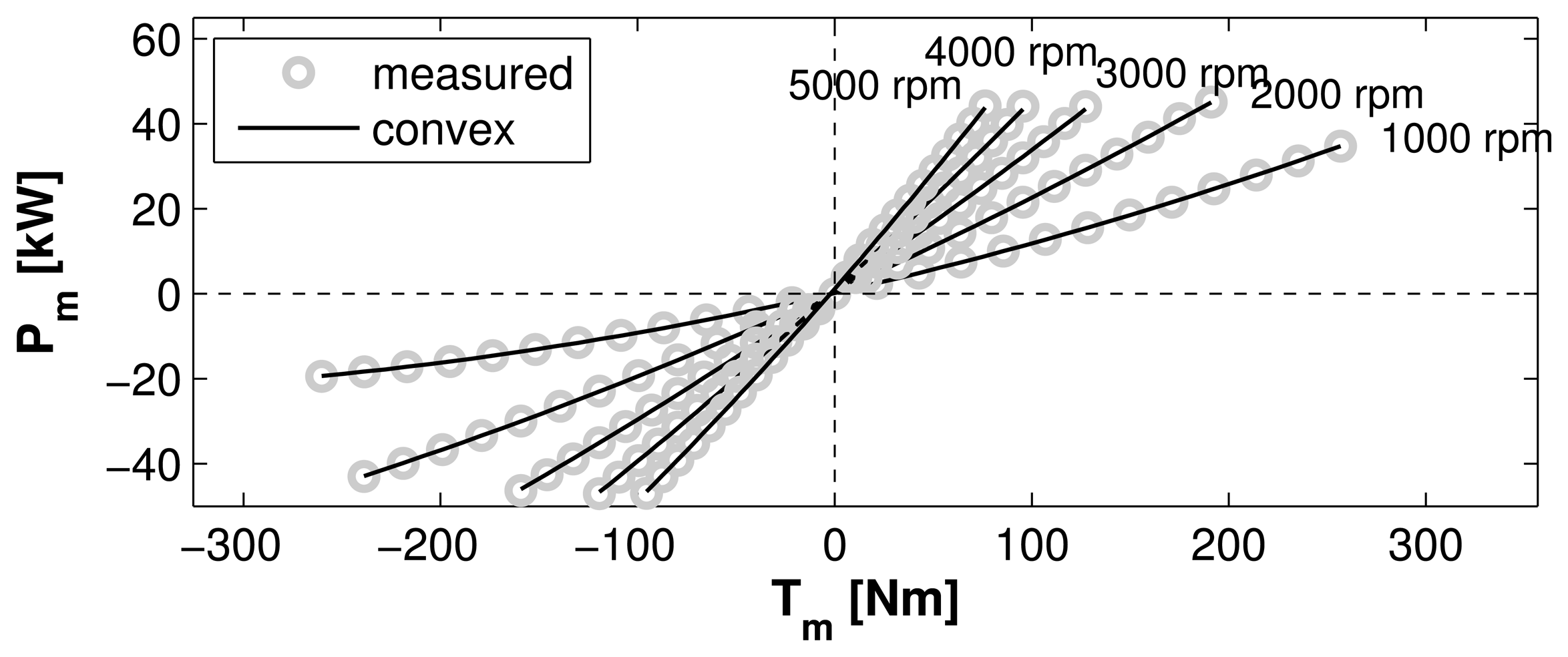
The electric motor, with a nominal power of 40 kW, is directly coupled to the input shaft of the gearbox such that the motor speed ω_m is always equal to ω_g. The power of the electric motor including the power electronics is approximated by a second-order polynomial with speed-dependent coefficients (the time index k being neglected for readability):

$$P_m\ge b_0({\omega }_m)+b_1({\omega }_m)T_m+b_2({\omega }_m)T_m^2$$

(8)

This description is convex in the variable T_m, which is required in the convex optimization problem in Equation (27) introduced later. Although Equation (8) potentially allows for wasting of the electrical energy, the optimal solution will always hold with equality [29].

The operation of the motor is limited by its minimum and maximum torque limitations, as well as by its maximum speed:

$$0\le {\omega }_m(k)\le {\omega }_{m,\mathit{\text{max}}}$$

(9)

$$T_{m,\mathit{\text{min}}}({\omega }_m(k))\le T_m(k)\le T_{m,\mathit{\text{max}}}({\omega }_m(k))$$

(10)

The model fit for the electric motor compared to the underlying measurement data is shown in Figure 2. The measurement data were obtained for a 25 kW permanent magnet synchronous motor. The torque axis is then linearly scaled with the nominal power while the efficiencies are kept constant. For more information on the scaling method, see for instance [21,49]. Clearly, the fit is very good in the entire operating range.

2.6. Engine Model

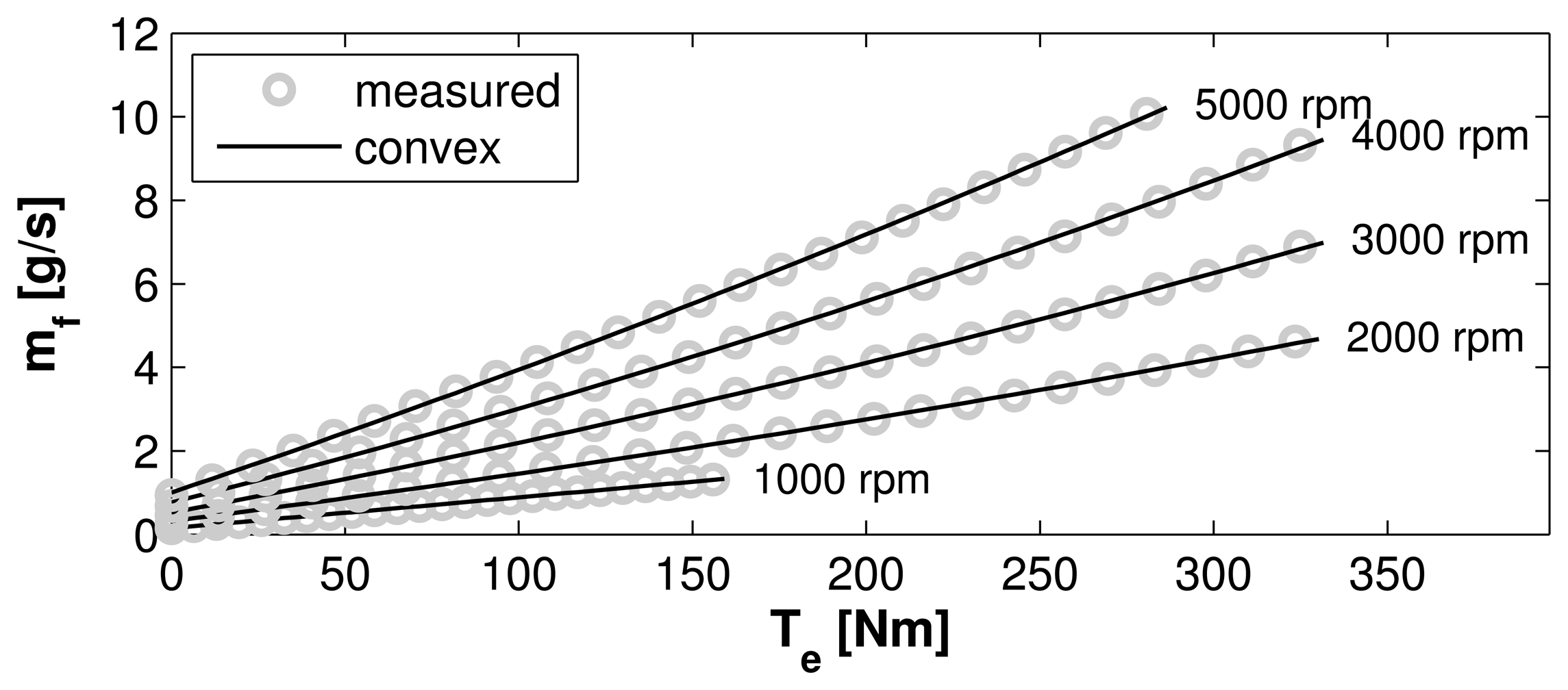
The mass flow ṁ_f of the fuel consumed is approximated by a second-order polynomial with speed-dependent coefficients (the time index k being neglected):

$${\dot{m}}_f\ge a_0({\omega }_e)+a_1({\omega }_e)T_e+a_2({\omega }_e)T_e^2$$

(11)

where ω_e denotes the rotational speed of the engine. This description is convex in the variable T_e, which is needed in the convex optimization problem in Equation (27) introduced later.

At all times, the engine is only allowed to operate within its limits defined by a maximum torque, minimum speed and a maximum speed condition, i.e.,

$${\omega }_{e,\mathit{\text{min}}}\le {\omega }_e(k)\le {\omega }_{e,\mathit{\text{max}}}$$

(12)

$$0\le T_e(k)\le T_e({\omega }_e(k))$$

(13)

The model fit of the engine compared to measurement data is shown in Figure 3. The measurement data were obtained for a modern 125 kW turbocharged spark-ignited combustion engine. The torque axis is then linearly scaled with the nominal power while the efficiencies are kept constant. For more information on the scaling method, see for instance [21,49]. The fit is good, with only small errors at high torques at high speeds.

The engine on/off decision is determined via the variable u_e ∈ {0,1} such that the engine state e is dictated by:

$$e(k)=u_e(k)$$

(14)

here, the value e = 1 represents the “on” state; and e = 0 represents the “off” state. If the engine is on, the engine speed is equal to w_g, unless the first gear is engaged, where the clutch is allowed to slip. If the engine is off, the engine speed is equal to zero, and the engine is disconnected from the rest of the powertrain. Moreover, each engine start is assumed to consume m_e = 0.3 g fuel equivalent, i.e.,

$$m_e(k)=\{\begin{array}{ll}0.3\text{g}\hfill & \text{if}e(k)=1\text{and}e(k-1)=0\hfill \\ 0\hfill & \text{else}\hfill \end{array}$$

(15)

These start costs represent the fuel-equivalent costs to start the engine. For example, these costs can be calculated based on an electrical energy consumption to crank up the engine to its start speed and a fuel consumption to synchronize the engine speed with the gearbox input speed, see for instance [39,48]. In the optimization, artificial costs can be assigned in order to reduce frequent engine starts. For the method proposed in this paper, the type of loss model is not restricted to the form Equation (15). A more detailed start model [39,48] could also be employed because the engine on/off decision is not assumed to be convex.

2.7. Battery Model

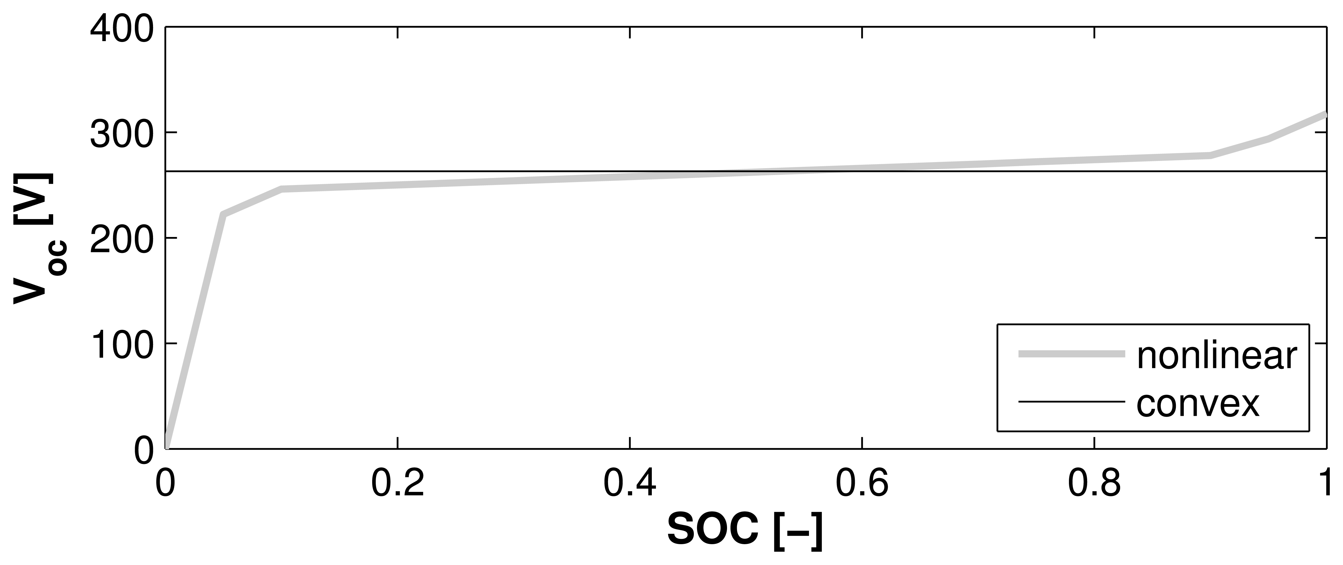
The battery is assumed to be of the LiFePO₄ type [50,51] with the data taken from [29]. It is modeled as an equivalent circuit with an open-circuit voltage V_oc in series with a constant internal resistance R_i [1]. In the nonlinear model, the open-circuit voltage is a function of the SOC as shown in Figure 4. In the convex model, the open-circuit voltage is assumed to be constant. The assumptions of a constant open-circuit voltage and a constant resistance are reasonable in the typical operating range of the battery [2,17,28,34]. Figure 4 shows a comparison of the two models.

In the convex case, the discrete-time equation of the dynamics for the battery SOC reads:

$$\mathit{\text{SOC}}(k+1)=\mathit{\text{SOC}}(k)-\mathrm{\Delta }t\cdot \frac{I_b(k)}{Q_0}$$

(16)

$$I_b(k)=\frac{V_{oc}-\sqrt{V_{oc}^2-4R_i(P_m(k)+P_{\mathit{\text{aux}}})}}{2\cdot R_i}$$

(17)

where I_b is the battery current, P_aux is a constant power consumed by electric auxiliary units, and Δt is the constant sampling time of 1 s. Equation (16) is convex in SOC and in I_b, however, Equation (17) has to be reformulated to:

$$P_m(k)\le V_{oc}\cdot I_b(k)-R_i\cdot I_b^2(k)-P_{\mathit{\text{aux}}}$$

(18)

in order to be convex in the optimization variable of interest, which here is I_b only.

The battery current and the battery SOC are constrained to:

$$I_{b,\text{min}}\le I_b(k)\le I_{b,\mathit{\text{max}}}$$

(19)

$${\mathit{\text{SOC}}}_{\mathit{\text{min}}}\le \mathit{\text{SOC}}(k)\le {\mathit{\text{SOC}}}_{\mathit{\text{max}}}$$

(20)

respectively.

2.8. Overview

In summary, the control variables u and the states x of the dynamical system are given by:

$$u(k)\triangleq \left[\begin{array}{l}{u}_g(k)\hfill \\ u_e(k)\hfill \\ u_{ts}(k)\hfill \end{array}\right]$$

(21)

$$x(k)\triangleq \left[\begin{array}{c}\mathit{\text{SOC}}(k)\\ g(k)\\ e(k)\end{array}\right]$$

(22)

3. Problem Formulation

The problem to be solved is the energy management problem formulated as an optimal control problem as follows:

$$\underset{u(k),k\in \{1,\dots ,N\}}{min}\sum _{k=1}^N({\dot{m}}_f(k)\cdot \mathrm{\Delta }t+m_g(k)+m_e(k))$$

(23)

subject to the vehicle model in Equations (1)–(22) and subject to the charge-sustenance condition SOC(N + 1) = SOC(1) = SOC₀ with SOC₀ being the initial state of charge.

The energy management problem can be solved using DP. However, to account for the engine start and gearshift losses, three state variables are required, i.e., the battery SOC, the engine state, and the gear currently engaged. Unfortunately, the computation time of this pure DP approach is large even for a coarse discretization for the SOC. Moreover, the accuracy of the solution is influenced by the discretization of the problem.

A more efficient approach to solve the problem was proposed in [41] where DP and PMP are combined such that the SOC state can be removed from the DP. As such, DP optimizes the equivalent fuel consumption for a given equivalence factor and for given engine start and gearshift costs, and the optimal solution is found by iterating on the equivalence factor until a charge sustaining solution is found. The advantage of this solution is the fact that the algorithm finds a close-to-optimal solution in a relatively short amount of time. Its main drawback is the fact that finding a charge-sustaining equivalence factor cannot be guaranteed, and therefore a heuristic approach has to be used instead. Another drawback consists of the fact that state constraints on the SOC cannot be handled.

In this paper, these drawbacks are avoided by extending the ideas presented in [41]. Accordingly, convex optimization is used to find a charge-sustaining equivalence factor and to handle the state constraints, while DP is used to find the optimal engine on/off and gearshift strategy.

4. Iterative Algorithm

As shown in [41], by application of PMP, the optimal control problem (23) can be reformulated to

$$\underset{u(k),s(k),k\in \{1,\dots ,N\}}{min}\sum _{k=1}^N\left({\dot{m}}_f(k)\cdot \mathrm{\Delta }t+s(k)\cdot I_b(k)\cdot V_{oc}\cdot \mathrm{\Delta }t+m_g(k)+m_e(k)\right)$$

(24)

with s denoting the equivalence factor between fuel consumption and electrical energy consumption. This equivalence factor is basically the Lagrange multiplier of the Euler-Lagrange formulation of the optimal control problem, sometimes also referred to as the dual variable. The dynamics of s are given by the necessary conditions of PMP. If the SOC dynamics are independent of the SOC, then s can be shown to be piecewise constant [52]. If in addition no state constraints are present on the SOC, s is constant for the entire driving cycle. The ultimate goal is then to find the optimal trajectory of s resulting in a charge-sustaining solution. As shown in the following, the aforementioned properties can be used to derive an efficient algorithm.

By further defining:

$$H(k,u(k),s(k))\triangleq {\dot{m}}_f(k)\cdot \mathrm{\Delta }t+s(k)\cdot I_b(k)\cdot V_{oc}\cdot \mathrm{\Delta }t$$

(25)

the authors of [41] showed that Equation (24) is equal to:

$$\underset{\begin{array}{c}{u}_g(k),u_e(k),s(k)\\ k\in \{1,\dots ,N\}\end{array}}{min}\sum _{k=1}^N\left(\underset{u_{ts}}{min}(H(k,u(k),s(k)))+m_g(k)+m_e(k)\right)$$

(26)

i.e., by instantaneously minimizing the function H(.), the optimal torque split u_ts can be found immediately for a given combination of u_g and u_e. Therefore, if the charge-sustaining value of s is known, problem in Equation (26) can be solved with DP using the gear g and the engine state e as the only state variables. The problem then remains to find the charge-sustaining value of s which, in [41], is effected by a root finding algorithm. However, that method does not yield optimal results if state constraints on the SOC are present or if engine start costs are considered. The reason is that in those cases, it is not possible to find the optimal equivalence factor s using a root finding algorithm because s is not constant.

Therefore, in this paper, the difference to the approach described in [41] is the fact that the equivalence factor is determined by solving a convex optimization problem instead of applying a root finding algorithm. The convex optimization problem to be solved is formulated as follows (bold symbols represent optimization variables):

Minimize:

$$\sum _{k=1}^N{\dot{\mathit{\text{m}}}}_f(k)\cdot \mathrm{\Delta }t$$

(27a)

subject to:

$${\mathit{\text{P}}}_m(k)\le V_{oc}\cdot {\mathit{\text{I}}}_b(k)-R_i\cdot {\mathit{\text{I}}}_b^2(k)-P_{\mathit{\text{aux}}}$$

(27b)

$${\dot{\mathit{\text{m}}}}_f(k)\ge u_e(k)\cdot \left(a_0(k)+a_1(k)\cdot {\mathit{\text{T}}}_e(k)+a_2(k)\cdot {\mathit{\text{T}}}_e^2(k)\right)$$

(27c)

$$T_g(k)={\mathit{\text{T}}}_m(k)+u_e(k)\cdot {\mathit{\text{T}}}_e(k)$$

(27d)

$${\mathit{\text{P}}}_m(k)\ge b_0(k)+b_1(k)\cdot {\mathit{\text{T}}}_m(k)+b_2(k)\cdot {\mathit{\text{T}}}_m^2(k)$$

(27e)

$$\mathit{\text{SOC}}(k+1)=\mathit{\text{SOC}}(k)-\mathrm{\Delta }t\cdot \frac{{\mathit{\text{I}}}_b(k)}{Q_0}$$

(27f)

$${\mathit{\text{T}}}_m(k)\ge T_{m,\mathit{\text{min}}}(k)$$

(27g)

$${\mathit{\text{T}}}_m(k)\le T_{m,\mathit{\text{max}}}(k)$$

(27h)

$${\mathit{\text{T}}}_e(k)\ge 0$$

(27i)

$${\mathit{\text{T}}}_e(k)\le T_{e,\mathit{\text{max}}}(k)$$

(27j)

$${\mathit{\text{I}}}_b(k)\ge I_{b,\mathit{\text{min}}}$$

(27k)

$${\mathit{\text{I}}}_b(k)\le I_{b,\mathit{\text{max}}}$$

(27l)

$$\mathit{\text{SOC}}(k)\ge {\mathit{\text{SOC}}}_{\mathit{\text{min}}}$$

(27m)

$$\mathit{\text{SOC}}(k)\le {\mathit{\text{SOC}}}_{\mathit{\text{max}}}$$

(27n)

$$\mathit{\text{SOC}}(1)={\mathit{\text{SOC}}}_0$$

(27o)

$$\mathit{\text{SOC}}(N+1)={\mathit{\text{SOC}}}_0$$

(27p)

for all k ∈ {1, …, N}.

Note that the gearshift and engine on/off sequence must be defined prior to solving Equation (27), otherwise the problem is not convex. As a consequence, the gearbox torque T_g(k) and the speeds ω_e(k) and ω_g(k) can be precalculated for the entire driving cycle.

The problem in Equation (27) is parsed with CVX [53] and solved with SeDuMi [54]. As a result, CVX yields the dual variable associated with Equation (27f). In this case, the dual variable is identical the equivalence factor s.

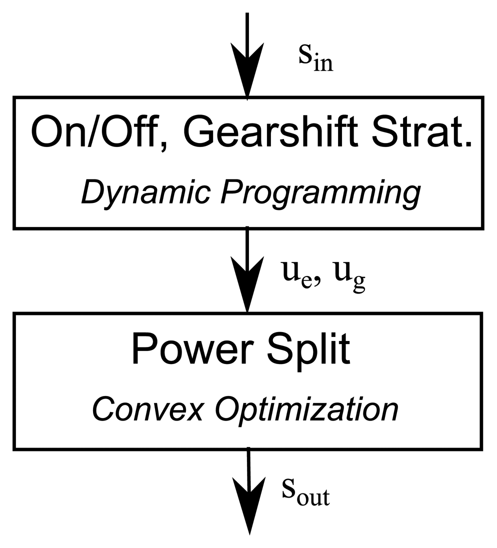
As illustrated in Figure 5, the above ideas are combined to perform a sequential optimization of the engine on/off and of the gearshift strategy using DP and the power split strategy using convex optimization. The input to the DP is the equivalence factor s_in, and the output of the DP consists of the gearshift strategy u_g and the engine on/off strategy u_e. Here, s_in stands for s_in(k) ∀k ∈ {1, …, N}. A similar notation is used for s, s_out, u_e, u_g. In a next step, a new equivalence factor s_out is calculated by solving the convex optimization problem in Equation (27) for the previously calculated values of u_g and u_e.

Assuming that the optimal value of s_in = s^⋆ is known, the optimal values of $u_g^{\star }$ and $u_e^{\star }$ are obtained by using DP [41]. The symbol ^⋆ stands for optimal, and ≡ stands for identity of the trajectory. On the other hand, solving the convex problem for the optimal values of $u_g^{\star }$ and $u_e^{\star }$ yields the optimal value of s_out ≡ s^⋆ [30,34]. Therefore, if s_in ≡ s^⋆, then s_out ≡ s_in ≡ s^⋆. As a consequence, the identity “s_out ≡ s_in” is a necessary condition for the optimality of a solution.

To show that this condition is also a sufficient condition, the condition “if and only if s_out ≡ s_in ⇒ s_out ≡ s^⋆” has to be shown. To do so, two further scenarios need to be considered for the case if s_in ≠ s^⋆: in the first scenario, it may happen that solving Equation (26) yields $u_g^{\star }$ and $u_e^{\star }$ although s_in ≠ s^⋆ (for example if the torque split strategy is not optimal). Therefore, the conclusion follows that solving Equation (27) yields s_out ≡ s^⋆, and therefore s_out ≠ s_in.

In the second scenario, solving Equation (26) yields $u_g\ne u_g^{\star }$ and/or $u_e\ne u_e^{\star }$. Then, solving Equation (27) results in s_out ≠ s^⋆ and also s_out ≠ s_in as explained in the following:

Assume that the values of s_in are lower than those of the optimal solution s^⋆. This means that electric energy is considered to be cheap in the optimization problem in Equation (26). Hence, the solution to Equation (26) results in an energy management strategy (i.e., u_ts, u_g, u_e) in which the vehicle is operated in the pure electric mode for more time, implying also that the engine is used less than in the optimal solution. “Using the engine less” means that recharging the battery via operating point shifting is done at lower additional loads than optimal, but also that the total engine runtime is less than optimal. Therefore, the SOC is not sustained over the entire driving cycle.

Then, at the next step of the sequential optimization, the optimal power split is calculated via convex optimization for the values of u_e and u_g obtained at the previous step. Since the solver for the convex problem in Equation (27) tries to find an SOC sustaining solution for the given engine runtime that is lower than optimal, the engine has to be operated at higher loads to generate more electric energy during the intervals where the engine is on. In the optimization problem in Equation (27), an increased use of the engine can only be achieved by considering the electric energy to be expensive, requiring the values of the equivalence factor s_out to be higher than those of s_in. Therefore, if s_in ≠ s^⋆, then s_out ≠ s_in. Finally, it is concluded that if and only if s_out ≡ s_in holds, then s_out ≡ s^⋆.

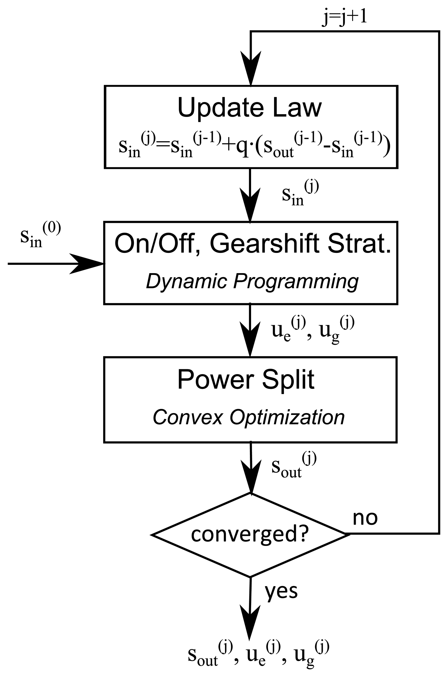
Based on these arguments, an iterative algorithm can be constructed which starts with an initial guess of s_in and converges towards a solution which fulfills the condition s_in≡ s_out. In the following, this iterative algorithm is referred to as the DP-C method. Figure 6 illustrates the entire DP-C method which is explained in detail below.

Step 1: Initialization of the algorithm

The iteration counter is initialized by j = 0. The initial equivalence factor $s_{\text{in}}^{(0)}$ is initialized by a constant value for the entire driving cycle. In the case studies below, a constant value of 2.9 is chosen. Notice that in the simulation results below, instead of the fuel mass flow the fuel power is optimized. More details are given in the Results Section below. Alternatively, some initial engine on/off strategy $u_e^{(-1)}$ and gearshift strategy $u_g^{(-1)}$ can be chosen to obtain an initial value $s_{\text{in}}^{(0)}$ by solving the convex problem in Equation (27).

Step 2: Use of DP to obtain $u_g^{(j)}$, $u_e^{(j)}$

In this step, based on $s_{\text{in}}^{(j)}$, DP is employed to solve Equation (26). Notice that in total only two states are needed, namely one for the gear and one for the engine on/off state. A state for the battery SOC is not included, allowing the DP problem for a typical driving mission to be solved in less than a second on a notebook with an Intel Core i7 CPU 64-bit with 2.80 GHz.

As a result, new values of $u_g^{(j)}$ and $u_e^{(j)}$ are obtained which are optimal for $s_{\text{in}}^{(j)}$. However, the solution does not guarantee charge sustenance since in this step, the state for the SOC and the corresponding final state constraint were removed from the problem.

Step 3: Use of convex optimization to obtain $s_{\mathbf{\text{out}}}^{(j)}$

For the given values of $u_g^{(j)}$ and $u_e^{(j)}$, the power split is calculated by solving Equation (27). As a result, the charge-sustaining equivalence factor $s_{\text{out}}^{(j)}$ is obtained.

Step 4: Check for convergence

To check whether the DP-C method has converged, the trajectories of $s_{\text{in}}^{(j)}$ and $s_{\text{out}}^{(j)}$ are compared by calculating the root mean square error:

$$E=\sqrt{\frac{1}{N}\sum _{k=1}^N{\left(s_{\text{in}}{\left(k\right)}^{(j)}-s_{\text{out}}{\left(k\right)}^{(j)}\right)}^2}$$

(28)

If the value of E is lower than some predefined tolerance E_TOL, the iteration is terminated and the results can be returned. If the value of E is larger than E_TOL, the iteration counter is updated by j ← j + 1, and the update law described in Step 5 below is applied.

In practice, it is more convenient to define a convergence tolerance ΔFC_TOL for the fuel consumption and the additional condition that u_g and u_e do not change between any two consecutive iterations. For the case studies below, this stopping criterion was used with ΔFC_TOL = 1 × 10⁻⁵ L/100 km. However, this method of checking the convergence is not equivalent to the one described in the first paragraph above. Therefore, checking whether E decreases at each iteration is recommended.

Step 5: Update law

Performing Steps 2 and 3 does not necessarily yield the optimal solution since the optimal equivalence factor is unknown. Initializing the equivalence factor s_in with a too high value will result in a too low value for s_out (and vice versa), as explained above. Therefore, the optimal s^⋆ lies between s_in and s_out. To ensure convergence towards s^⋆, damping is introduced by including an update law for the equivalence factor $s_{\text{in}}^{(j)}$ before step 2. The update law used here is taken from [30], which is:

$$s_{\text{in}}^{(j)}=s_{\text{in}}^{(j-1)}+q\cdot (s_{\text{out}}^{(j-1)}-s_{\text{in}}^{(j-1)})$$

(29)

with the convergence parameter q. The value of the convergence parameter is initially chosen as q = 0.2. When the change of the root mean square error Equation (28) between any two consecutive iterations falls below a certain threshold value, the convergence parameter is reduced by q ← 0.7 · q. By using this update law, $s_{\text{out}}^{(j)}$ converges towards s^⋆ for j → ∞.

By using the tolerance criterion introduced in Step 4 (ΔFC_TOL), the algorithm terminates after two to ten iterations, depending on the driving cycle and the initial value for the equivalence factor.

5. Results

For the generation of the optimization results shown below, the indicator for the fuel consumption in Equation (27a) is replaced by the fuel power P_f which is defined by

$$P_f={\dot{m}}_f\cdot H_l$$

(30)

with H_l being the lower heating value of the fuel. The fuel power allows for a more intuitive interpretation of the equivalence factor s since it then “converts battery power to an equivalent fuel power that must be added to the actual fuel power to attain a charge-sustaining control strategy” [2] (p. 66). The resulting values for the equivalence factor can also be compared more easily to those found in the literature.

5.1. Performance Comparison with the Convex Vehicle Model

To assess the performance of the DP-C method, it is compared to a pure DP implementation of the convex vehicle model described in Section 2. For the following case studies, unless stated otherwise, the minimum and maximum values of the SOC are assumed to be 20% and 80%, respectively. The SOC state of the DP method is discretized with a resolution of 1% SOC.

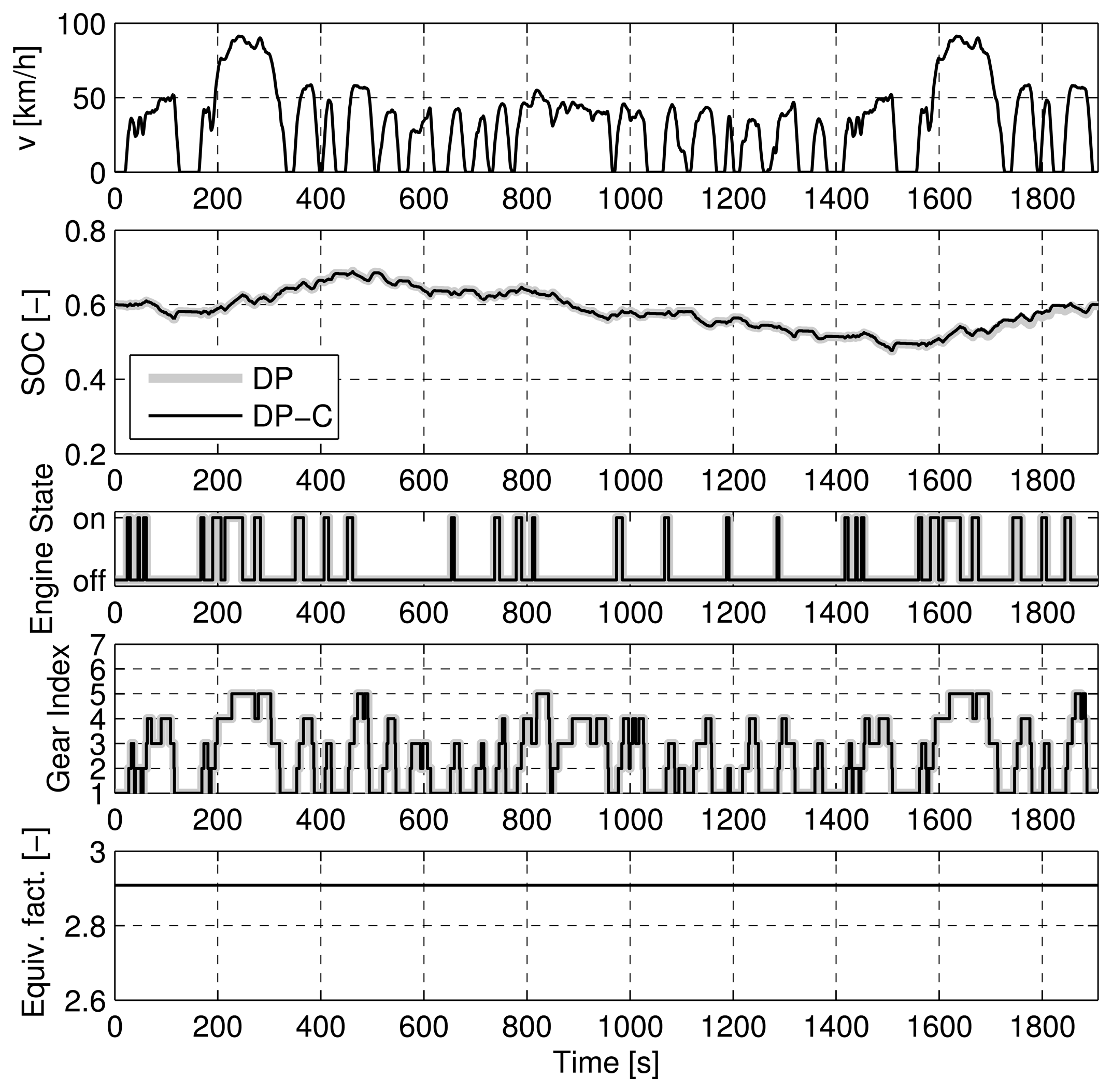
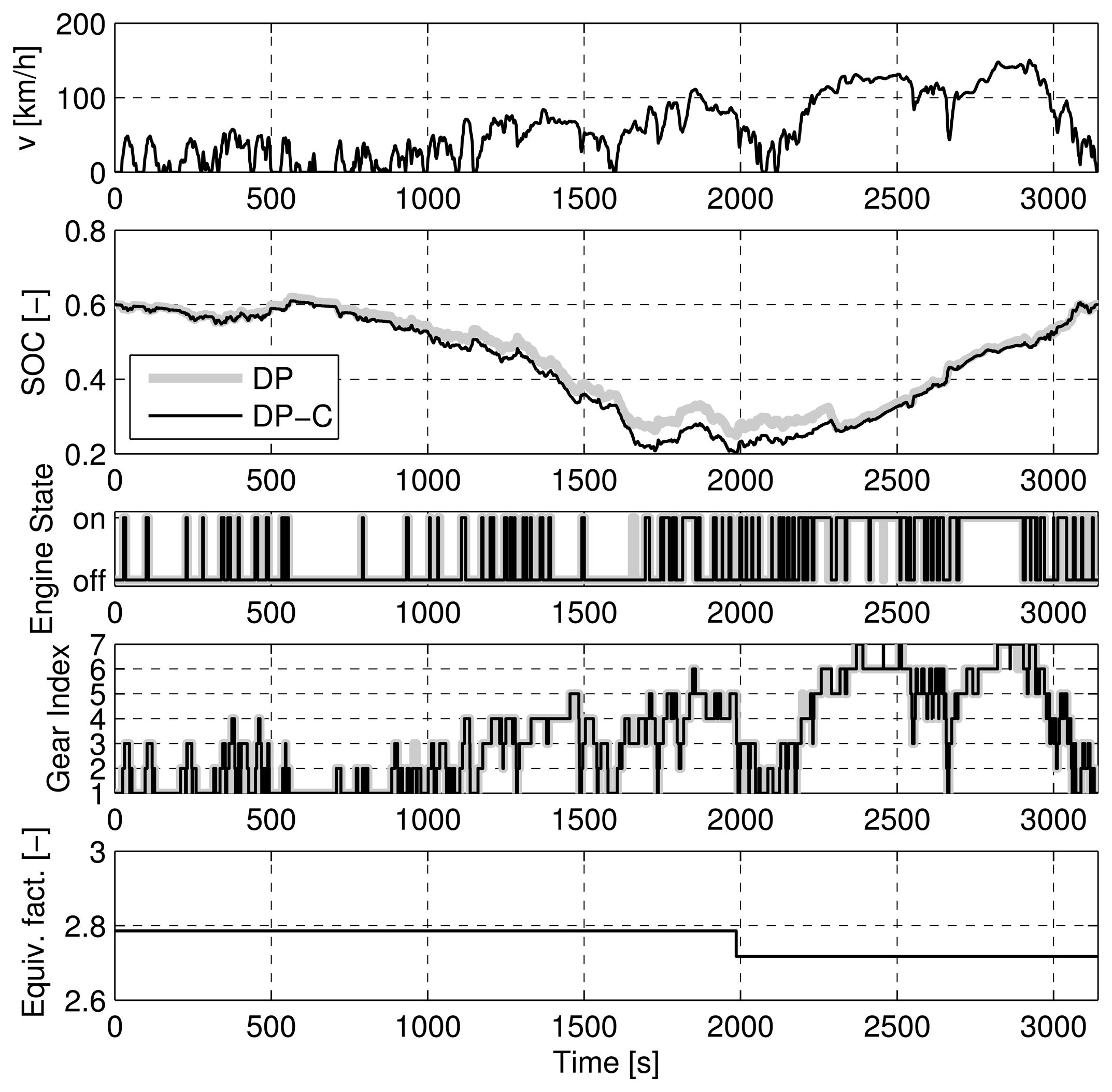
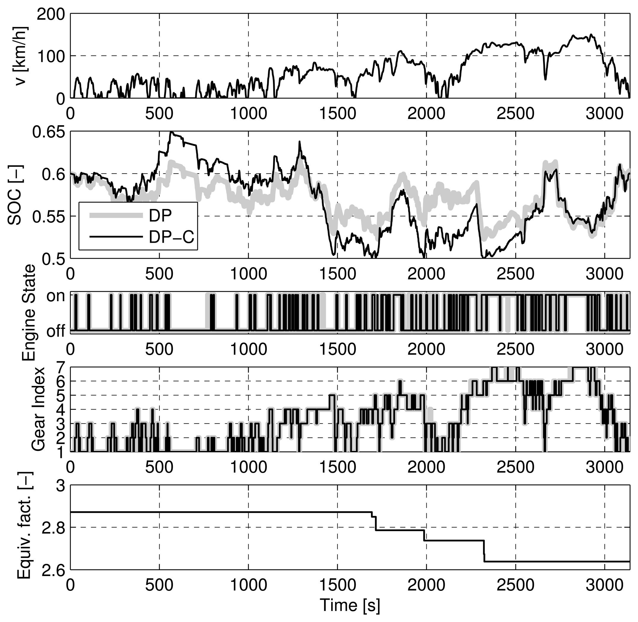
Both the DP-C and the DP method are applied on three well-known driving cycles, namely the New European Driving Cycle (NEDC), the Federal Test Procedure (FTP), and the Common Artemis Driving Cycle (CADC). In a further case, referred to as “CADC bounded”, the DP-C and the DP method are both applied to the CADC with tighter SOC constraints, i.e., 0.50 ≤ SOC ≤ 0.65.

Table 2. Results with the convex vehicle model.

Cycle	Performance Index	DP	DP-C	Difference
NEDC	FC [L/100 km]	4.405	4.399	(−0.1%)
	ICE starts [#]	7	7	(+0.0%)
	Gearshifts [#]	86	86	(+0.0%)
	CPU time [s]	791	6	(−99.2%)
FTP	FC [L/100 km]	4.288	4.279	(−0.2%)
	ICE starts [#]	28	28	(+0.0%)
	Gearshifts [#]	180	182	(+1.1%)
	CPU time [s]	1287	14	(−98.9%)
CADC	FC [L/100 km]	5.635	5.627	(−0.1%)
	ICE starts [#]	78	75	(−3.8%)
	Gearshifts [#]	316	310	(−1.9%)
	CPU time [s]	2363	105	(−95.5%)
CADC (bounded)	FC [L/100 km]	5.657	5.643	(−0.2%)
	ICE starts [#]	90	85	(−5.6%)
	Gearshifts [#]	322	310	(−3.7%)
	CPU time [s]	527	122	(−76.9%)

summarizes the fuel consumption, the number of engine starts, the number of gearshifts, and the computation time for the four cases considered. The computation time was identified on a standard notebook with an Intel Core i7 CPU (64-bit, 2.80 GHz).

As Table 2 shows, the fuel consumption (FC) calculated by the DP-C method is always slightly lower than the one calculated by the DP method. The number of engine starts and the number of gearshifts are identical for both methods on the NEDC, whereas on the other driving cycles, these numbers are very similar. The differences are explained by the fact that the DP method requires a discretized state space for the continuous state of the SOC, whereas the DP-C method does not. The discretization of the SOC state for the DP method results in errors occurring during the interpolation of the cost-to-go function in the backward recursion of the DP. As a consequence, this cost-to-go function yields a sub-optimal control performance when compared to an ideal implementation. However, these discretization errors could only be reduced by increasing the resolution of the discretized state space, which would lead to an increased computational burden.

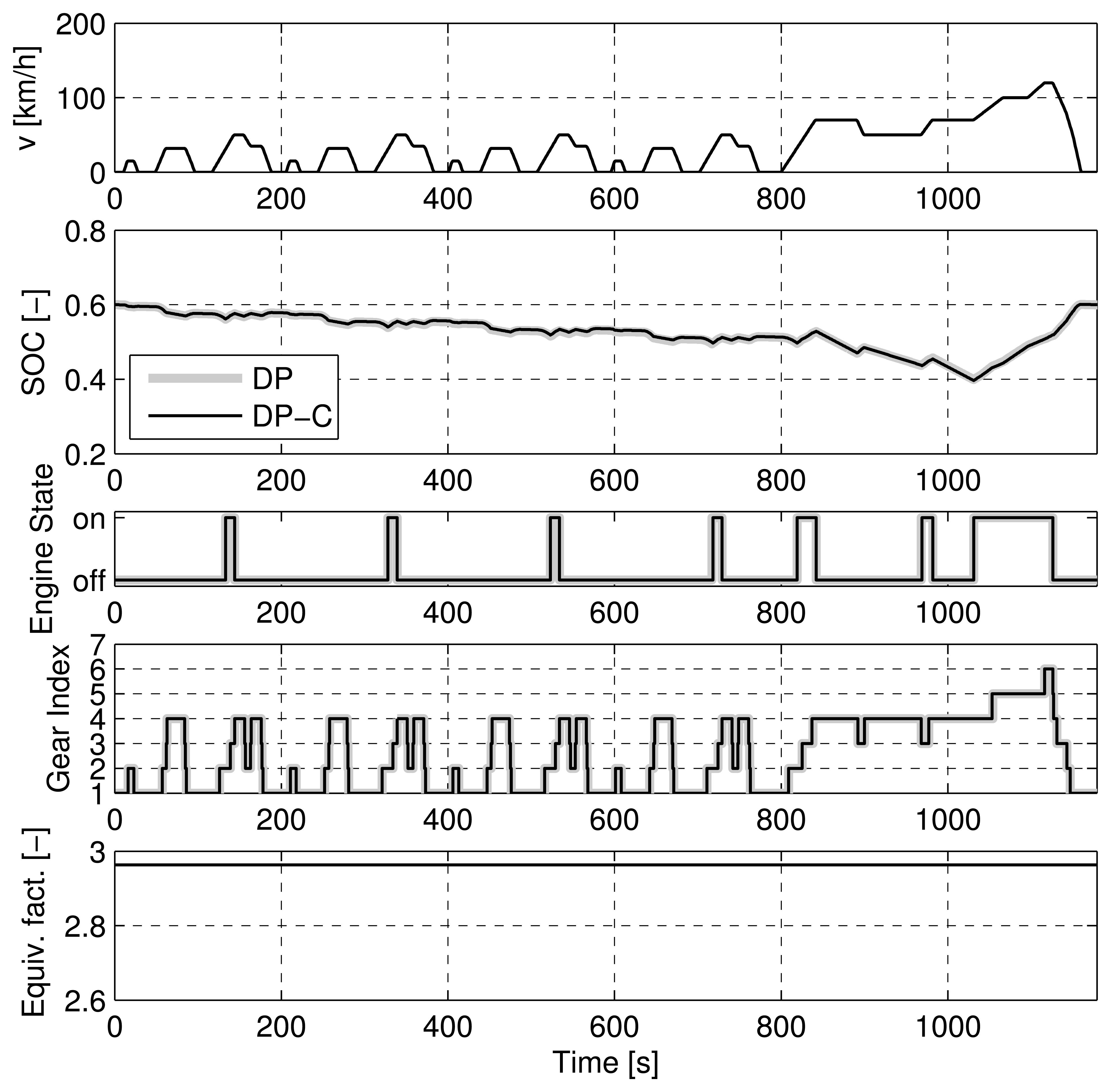
Figures 7, 8, 9, and 10 show the trajectories of the SOC, engine on/off state, the gear state, and the equivalence factor for the four cases considered above. For the NEDC (Figure 7) and the FTP (Figure 8), the trajectories show an almost perfect match of the DP-C and the DP methods (except for one up- and downshift in the FTP). For the two CADC cases, the trajectories do not match well. As described above, the mismatch is attributable to the error introduced by the discretization of the SOC state. Particularly at the border of the feasible state space, the interpolation errors between the feasible and the infeasible state space lead to an error in the cost-to-go function [47].

Comparing the computational burden associated with the DP-C and the DP methods, the DP-C significantly outperforms the DP method. As Table 2 shows, the DP-C method requires less than 10% of the time required by the DP method. In the case of the “CADC bounded”, the DP-C method still requires only about 20% of the time required by the DP method, although a reduced number of discrete supporting points for the SOC state are used in the DP method.

Summarizing the findings described in this section, the DP-C method yields more accurate results in much less time than a pure DP implementation.

5.2. Performance Comparison with the Nonlinear Vehicle Model

To assess the performance of the DP-C method on the nonlinear vehicle model, the control strategy obtained with the DP-C method is applied to the nonlinear model. The result obtained is then compared to the result of a pure DP implementation including the nonlinear model. In this case study, the only differences of the nonlinear model compared to the convex model are the use of the original consumption maps instead of second-order polynomials in Equations (8) and (11), as well as the use of the nonlinear open-circuit voltage characteristic presented in Figure 4.

To increase the accuracy of the DP-C method on the nonlinear vehicle model, the DP-C algorithm is modified at Step 2 (“DP for u_g and u_e”): Instead of using the convex vehicle model, the nonlinear model is used. The advantage of this modification results in a more accurate gearshift and engine on/off strategy than in the case where the convex model is used. Therefore, the engine on/off and gearshift strategies can be different from those in the corresponding convex case.

As

Table 3. Results with the nonlinear vehicle model.

Cycle	Performance Index	DP	DP-C	Difference
NEDC	FC [L/100 km]	4.453	4.449	(−0.1%)
	ICE starts [#]	7	7	(+0.0%)
	Gearshifts [#]	56	54	(−3.6%)
	CPU time [s]	684	18	(−97.4%)
FTP	FC [L/100 km]	4.317	4.270	(−1.1%)
	ICE starts [#]	28	28	(+0.0%)
	Gearshifts [#]	138	138	(+0.0%)
	CPU time [s]	1111	17	(−98.5%)
CADC	FC [L/100 km]	5.625	5.642	(+0.3%)
	ICE starts [#]	84	74	(−11.9%)
	Gearshifts [#]	354	350	(−1.1%)
	CPU time [s]	1959	155	(−92.1%)
CADC (bounded)	FC [L/100 km]	5.639	5.654	(+0.3%)
	ICE starts [#]	93	88	(−5.4%)
	Gearshifts [#]	366	394	(+7.7%)
	CPU time [s]	434	107	(−75.5%)

shows for the NEDC and the FTP driving cycles, the fuel consumption obtained with the DP-C method can still be lower than the amount calculated with DP even for the nonlinear model. However, in the cases of the CADC and “CADC bounded”, the fuel consumption obtained by applying the DP-C method is higher by 0.3% than that calculated with DP. The degraded performance in fuel consumption of the DP-C method on the nonlinear model compared to the performance on the convex model is a direct consequence of the model approximations required to solve the convex problem in Equation (27). Nonetheless, the results obtained with the DP-C method are still quite acceptable.

In terms of computation time, the DP-C method is more than 90% faster than the DP method in the cases where the full range of the SOC is discretized (NEDC, FTP, CADC), and it is 75% faster in the case with the reduced SOC discretization (CADC bounded).

In conclusion, even for the nonlinear model, the DP-C method is able to yield close-to-optimal results in much less time than the pure DP method.

6. Discussion

6.1. Accuracy of the DP Method

In the case of the convex model, the above values for the fuel consumption calculated by DP are always worse than those obtained with the DP-C method. The accuracy of the DP solutions could generally be improved by increasing the resolution of the discretization of the SOC state. However, the improvements in accuracy are very small compared to the additional computational burden required.

6.2. Advantages and Disadvantages of the DP-C Method

A substantial advantage of the DP-C method is its ability to yield globally optimal results for the convex vehicle model much faster than the DP method. In the case of a nonlinear model, the performance of the DP-C method is very close to that of the DP method. Moreover, the equivalence factor related to the battery state is obtained directly from the convex solver without any error-prone calculation via the optimal cost-to-go from DP. Furthermore, more accurate results can be obtained with the DP-C method than with the DP method because no discretization of the SOC state is necessary. In addition, as opposed to the method presented in [41], DP-C is also able to handle state constraints, which means that it detects the jumps in the equivalence factor.

The only drawback of the DP-C method are the modeling errors introduced by the convex modeling of the powertrain. However, in the case of the HEV in this paper, the errors are small.

7. Conclusions

This paper presents a method to calculate the globally optimal energy management strategy for a parallel HEV on a given driving cycle taking into account penalties to avoid frequent engine start and/or gearshift events. The proposed method combines DP and convex optimization in an iterative scheme. The algorithm converges to the globally optimal solution after a few iterations. The optimal gearshift and engine on/off strategy is evaluated by DP while convex optimization is used to determine the optimal power split strategy. The proposed method delivers globally optimal results with respect to the convex vehicle model, even in the presence of state constraints. When compared to the basic DP algorithm, the proposed method results in a substantial reduction of the evaluation time.

For the convex vehicle model, the proposed method delivers a higher precision than DP (0.1%–0.2% lower fuel consumption) while incurring significantly less computational effort (75%–98% less). The higher precision is due to the fact that convex optimization does not require a discretization of the continuous control and state variables, which inherently introduces interpolation errors. To evaluate the magnitude of the error that is introduced by using convex model approximations, the strategy that was optimized for the convex model is applied to the nonlinear model. Compared to the true globally optimal solution obtained by applying DP on the nonlinear model, the proposed method results in a slight deterioration of precision only (up to 0.3% increased fuel consumption).

The proposed method can be extended to other vehicle topologies and different formulations of the energy management problem. For example, the battery state of health or the engine temperature could be considered by including further continuous state variables. Additional discrete state variables, such as for example the clutch state, as well as additional continuous and discrete control variables, such as for example the desired clutch state, the motor speed or torque of a series-parallel hybrid vehicle, could be included as well.

References

- Guzzella, L.; Sciarretta, A. Vehicle Propulsion Systems, 3rd ed.; Springer-Verlag: Berlin, Germany, 2013. [Google Scholar]
- Sciarretta, A.; Guzzella, L. Control of hybrid electric vehicles. IEEE Control Syst. Mag. 2007, 27, 60–70. [Google Scholar]
- Wipke, K.B.; Cuddy, M.R.; Burch, S.D. ADVISOR 2.1: A user-friendly advanced powertrain simulation using a combined backward/forward approach. IEEE Trans. Veh. Technol. 1999, 48, 1751–1761. [Google Scholar]
- Otsu, A.; Takeda, T.; Suzuki, O.; Hatanaka, K. Controlling Apparatus for a Hybrid Car. U.S. Patent 6,123,163, 26 September 2000. [Google Scholar]
- Lee, H.D.; Sul, S.K. Fuzzy-logic-based torque control strategy for parallel-type hybrid electric vehicle. IEEE Trans. Ind. Electron. 1998, 45, 625–632. [Google Scholar]
- Schouten, N.; Salman, M.; Kheir, N. Fuzzy logic control for parallel hybrid vehicles. IEEE Trans. Control Syst. Technol. 2002, 10, 460–468. [Google Scholar]
- Back, M.; Simons, M.; Kirschbaum, F.; Krebs, V. Predictive Control of Drivetrains. Proceedings of the International Federation of Automatic Control (IFAC) World Congress, Barcelona, Spain, 21–26 July 2002; Volume 15, pp. 1506–1506.
- Lin, C.C.; Peng, H.; Grizzle, J.W.; Kang, J.M. Power management strategy for a parallel hybrid electric truck. IEEE Trans. Control Syst. Technol. 2003, 11, 839–849. [Google Scholar]
- Pérez, L.V.; Bossio, G.R.; Moitre, D.; Garcia, G.O. Optimization of power management in an hybrid electric vehicle using dynamic programming. Math. Comput. Simul. 2006, 73, 244–254. [Google Scholar]
- Yuan, Z.; Teng, L.; Fengchun, S.; Peng, H. Comparative study of dynamic programming and pontryagins minimum principle on energy management for a parallel hybrid electric vehicle. Energies 2013, 6, 2305–2318. [Google Scholar]
- Zou, Y.; Sun, F.; Hu, X.; Guzzella, L.; Peng, H. Combined optimal sizing and control for a hybrid tracked vehicle. Energies 2012, 5, 4697–4710. [Google Scholar]
- Ngo, V.D.; Hofman, T.; Steinbuch, M.; Serrarens, A. Gear shift map design methodology for automotive transmissions. Proc. Inst. Mech. Eng. Part D J. Automob. Eng. 2013. [Google Scholar] [CrossRef]
- Ott, T.; Onder, C.; Guzzella, L. Hybrid-electric vehicle with natural gas-diesel engine. Energies 2013, 6, 3571–3592. [Google Scholar]
- Delprat, S.; Lauber, J.; Guerra, T.M.; Rimaux, J. Control of a parallel hybrid powertrain: Optimal control. IEEE Trans. Veh. Technol. 2004, 53, 872–881. [Google Scholar]
- Liu, J.; Peng, H. Modeling and control of a power-split. IEEE Trans. Control Syst. Technol. 2008, 16, 1242–1251. [Google Scholar]
- Serrao, L.; Onori, S.; Rizzoni, G. ECMS as a Realization of Pontryagin's Minimum Principle for HEV Control. Proceedings of the American Control Conference, St. Louis, MO, USA, 10–12 June 2009; pp. 3964–3969.
- Kim, N.; Cha, S.; Peng, H. Optimal control of hybrid electric vehicles based on pontryagin's minimum principle. IEEE Trans. Control Syst. Technol. 2011, 19, 1279–1287. [Google Scholar]
- Johnson, V.H.; Wipke, K.B.; Rausen, D.J. HEV control strategy for real-time optimization of fuel economy and emissions. SAE Trans. 2000, 109, 1677–1690. [Google Scholar]
- Musardo, C.; Rizzoni, G.; Staccia, B. A-ECMS: An Adaptive Algorithm for Hybrid Electric Vehicle Energy Management. Proceedings of the 44th IEEE Conference on Decision and Control, Seville, Spain, 12–15 December 2005; pp. 1816–1823.
- Chasse, A.; Sciarretta, A. Supervisory control of hybrid powertrains: An experimental benchmark of offline optimization and online energy management. Control Eng. Pract. 2011, 19, 1253–1265. [Google Scholar]
- Shankar, R.; Marco, J.; Assadian, F. The novel application of optimization and charge blended energy management control for component downsizing within a plug-in hybrid electric vehicle. Energies 2012, 5, 4892–4923. [Google Scholar]
- Lin, C.C.; Peng, H.; Grizzle, J.W. A Stochastic Control Strategy for Hybrid Electric Vehicles. Proceedings of the American Control Conference, Boston, MA, USA, 30 June–2 July 2004; Volume 5, pp. 4710–4715.
- Johannesson, L.; Asbogard, M.; Egardt, B. Assessing the potential of predictive control for hybrid vehicle powertrains using stochastic dynamic programming. IEEE Trans. Intell. Transp. Syst. 2007, 8, 71–83. [Google Scholar]
- Tate, E.D.; Grizzle, J.W.; Peng, H. Shortest path stochastic control for hybrid electric vehicles. Int. J. Robust Nonlinear Control 2008, 18, 1409–1429. [Google Scholar]
- Moura, S.J.; Stein, J.L.; Fathy, H.K. Battery-Health Conscious Power Management for Plug-in Hybrid Electric Vehicles via Stochastic Control. Proceedings of the ASME 2010 Dynamic Systems and Control Conference, Cambridge, MA, USA, 12–15 September 2010; pp. 615–624.
- Opila, D.F.; Wang, X.; McGee, R.; Gillespie, R.B.; Cook, J.A.; Grizzle, J.W. An energy management controller to optimally trade off fuel economy and drivability for hybrid vehicles. IEEE Trans. Control Syst. Technol. 2012, 20, 1490–1505. [Google Scholar]
- Boyd, S.P.; Vendenberghe, L. Convex Optimization; Cambridge University Press: New York, NY, USA, 2004. [Google Scholar]
- Murgovski, N.; Johannesson, L.; Hellgren, J.; Egardt, B.; Sjöberg, J. Convex Optimization of Charging Infrastructure Design and Component Sizing of a Plug-in Series HEV Powertrain. Proceedings of the 18th IFAC World Congress, Milan, Italy, 28 August–2 September 2011; pp. 13052–13057.
- Murgovski, N.; Johannesson, L.; Sjöberg, J.; Egardt, B. Component sizing of a plug-in hybrid electric powertrain via convex optimization. Mechatronics 2012, 22, 106–120. [Google Scholar]
- Elbert, P.; Nüesch, T.; Ritter, A.; Murgovski, N.; Guzzella, L. Engine on/off control for the energy management of a serial hybrid electric bus via convex optimization. IEEE Trans. Veh. Technol. 2014. [Google Scholar] [CrossRef]
- Hu, X.; Murgovski, N.; Johannesson, L.; Egardt, B. Energy efficiency analysis of a series plug-in hybrid electric bus with different energy management strategies and battery sizes. Appl. Energy 2013, 111, 1001–1009. [Google Scholar]
- Terwen, S.; Back, M.; Krebs, V. Predictive Powertrain Control for Heavy Duty Trucks. Proceedings of the 4th IFAC Symposium on Advances in Automotive Control, Salerno, Italy, 19–23 April 2004; pp. 105–110.
- Beck, R.; Bollig, A.; Abel, D. Comparison of two real-time predictive strategies for the optimal energy management of a hybrid electric vehicle. Oil Gas Sci. Technol. Rev. IFP 2007, 62, 635–643. [Google Scholar]
- Murgovski, N.; Johannesson, L.; Sjöberg, J. Engine on/off control for dimensioning hybrid electric powertrains via convex optimization. IEEE Trans. Veh. Technol. 2013, 62, 2949–2962. [Google Scholar]
- Paganelli, G.; Guerra, T.M.; Delprat, S.; Santin, J.J.; Delhom, M.; Combes, E. Simulation and assessment of power control strategies for a parallel hybrid car. Proc. Inst. Mech. Eng. Part D J. Automob. Eng. 2000, 214, 705–717. [Google Scholar]
- Delprat, S.; Guerra, T.; Rimaux, J. Control Strategies for Hybrid Vehicles: Optimal Control. Proceedings of the 56th IEEE Vehicular Technology Conference, Birmingham, AL, USA, 24–28 September 2002; Volume 3, pp. 1681–1685.
- Kleimaier, A.; Schröder, D. An Approach for the Online Optimized Control of a Hybrid Powertrain. Proceedings of the 7th International Workshop on Advanced Motion Control, Maribor, Slovenia, 3–5 July 2002; pp. 215–220.
- Sciarretta, A.; Back, M.; Guzzella, L. Optimal control of parallel hybrid electric vehicles. IEEE Trans. Control Syst. Technol. 2004, 12, 352–363. [Google Scholar]
- Ambühl, D. Energy Management Strategies for Hybrid Electric Vehicles. Ph.D. Thesis, ETH Zurich, Zurich, Switzerland, 2009. [Google Scholar]
- Vidal-Naquet, F.; Zito, G. Adapted Optimal Energy Management Strategy for Drivability. Proceedings of the IEEE Vehicle Power and Propulsion Conference, Seoul, Korea, 9–12 October 2012; pp. 358–363.
- Ngo, D.V.; Hofman, T.; Steinbuch, M.; Serrarens, A. Optimal control of the gear shift command for hybrid electric vehicles. IEEE Trans. Veh. Technol. 2012, 61, 3531–3543. [Google Scholar]
- Kolmanovsky, I.; Nieuwstadt, M.V. Optimization of Complex Powertrain Systems for Fuel Economy and Emissions. Proceedings of the IEEE International Conference on Control Applications, Kohala Coast, HI, USA, 22–27 August 1999; Volume 1, pp. 833–839.
- Murgovski, N.; Sjöberg, J.; Fredriksson, J. A methodology and a tool for evaluating hybrid electric powertrain configurations. Int. J. Electr. Hybrid Veh. 2011, 3, 219–245. [Google Scholar]
- Guzzella, L.; Amstutz, A. CAE tools for quasi-static modeling and optimization of hybrid powertrains. IEEE Trans. Veh. Technol. 1999, 48, 1762–1769. [Google Scholar]
- Murgovski, N.; Johannesson, L.; Sjöberg, J. Convex Modeling of Energy Buffers in Power Control Applications. Proceedings of the IFAC Workshop on Engine and Powertrain Control Simulation and Modeling, Rueil-Malmaison, France, 23–25 October 2012; pp. 92–99.
- Park, D.; Seo, T.; Lim, D.; Cho, H. Theoretical Investigation on Automatic Transmission Efficiency. Proceedings of the International Congress and Exposition, Detroit, MI, USA, 26–29 February 1996.
- Sundström, O.; Ambühl, D.; Guzzella, L. On implementation of dynamic programming for optimal control problems with final state constraints. Oil Gas Sci. Technol. Rev. IFP 2010, 65, 91–102. [Google Scholar]
- Ngo, D.V. Gear Shift Strategies for Automotive Transmissions. Ph.D. Thesis, Eindhoven University of Technology, Eindhoven, The Netherlands, 2012. [Google Scholar]
- Ebbesen, S.; Elbert, P.; Guzzella, L. Engine downsizing and electric hybridization under consideration of cost and drivability. Oil Gas Sci. Technol. Rev. IFP Energies Nouv. 2012, 68, 109–116. [Google Scholar]
- Nanophosphate High Power Lithium Ion Cell ANR26650M1-B; MD100113-01 Data Sheet; A123 Systems, Inc.: Waltham, MA, USA, 2011.
- Lee, J.; Yi, J.; Shin, C.; Yu, S.; Cho, W. Modeling the effects of the cathode composition of a lithium iron phosphate battery on the discharge behavior. Energies 2013, 6, 5597–5608. [Google Scholar]
- Geering, H.P. Optimal Control with Engineering Applications; Springer-Verlag: Berlin Heidelberg, Germany, 2007. [Google Scholar]
- Grant, M.; Boyd, S. CVX: Matlab Software for Disciplined Convex Programming (Web Page and Software). Available online: http://stanford.edu/~boyd/cvx (accessed on 11 March 2013).
- Sturm, J.F. Using SeDuMi 1.02, a MATLAB Toolbox for Optimization over Symmetric Cones. Optim. Methods Softw. 1999, 11, 625–653. [Google Scholar]