An Artificial Neural Network Compensated Output Feedback Power-Level Control for Modular High Temperature Gas-Cooled Reactors

Abstract

Small modular reactors (SMRs) could be beneficial in providing electricity power safely and also be viable for applications such as seawater desalination and heat production. Due to its inherent safety features, the modular high temperature gas-cooled reactor (MHTGR) has been seen as one of the best candidates for building SMR-based nuclear power plants. Since the MHTGR dynamics display high nonlinearity and parameter uncertainty, it is necessary to develop a nonlinear adaptive power-level control law which is not only beneficial to the safe, stable, efficient and autonomous operation of the MHTGR, but also easy to implement practically. In this paper, based on the concept of shifted-ectropy and the physically-based control design approach, it is proved theoretically that the simple proportional-differential (PD) output-feedback power-level control can provide asymptotic closed-loop stability. Then, based on the strong approximation capability of the multi-layer perceptron (MLP) artificial neural network (ANN), a compensator is established to suppress the negative influence caused by system parameter uncertainty. It is also proved that the MLP-compensated PD power-level control law constituted by an experientially-tuned PD regulator and this MLP-based compensator can guarantee bounded closed-loop stability. Numerical simulation results not only verify the theoretical results, but also illustrate the high performance of this MLP-compensated PD power-level controller in suppressing the oscillation of process variables caused by system parameter uncertainty.

1. Introduction

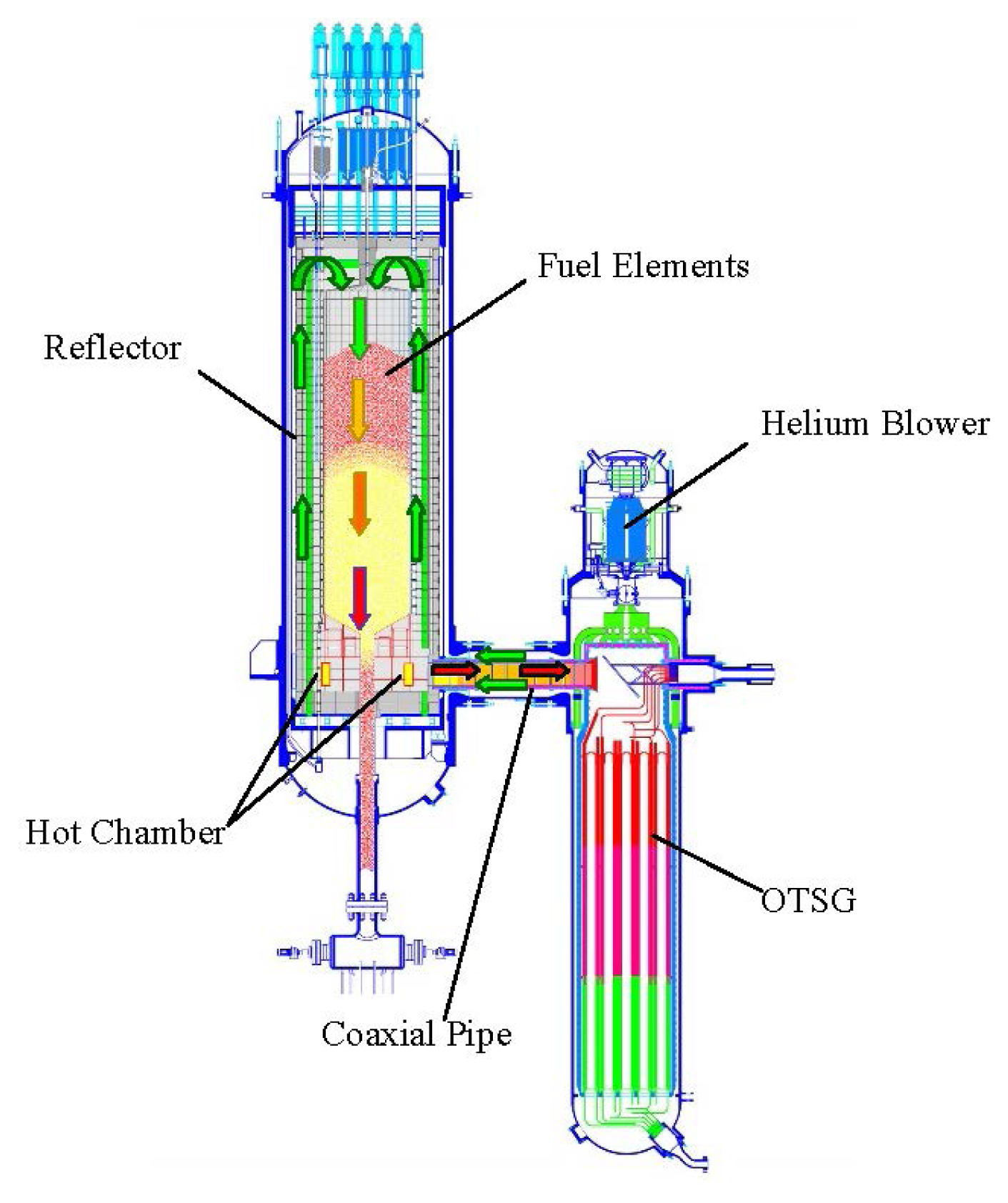
Nowadays, in addition to food and water, electricity is also a major factor that deeply influences human economic and social development. The increasing World population certainly results in an increased electricity demand. As a crucial type of clean energy, nuclear fission energy can play an important role in meeting the World's increasing energy needs. Small modular reactors (SMRs) are those nuclear fission reactors whose electrical output is less than 300 MW_e. Due to their passive safety, SMRs could be beneficial in providing electricity power to remote areas without transmission and distribution infrastructure and also be viable for specific localized applications such as seawater desalination and heat production [1,2]. The rated power of a SMR-based nuclear plant can be enlarged by adopting the scheme of multiple SMRs driving one turbine. Due to its inherent safety performance, the modular high temperature gas-cooled reactor (MHTGR, such as the HTR-MODUL designed in Germany and MHTGR designed in the US) has been seen as one of the best candidates for building SMR-based nuclear plants. The MHTGR uses helium as coolant and graphite as moderator and structural material, and its inherent safety is determined by the low power density, strong negative temperature feedback effect and slim reactor shape [3–5]. China began to study the MHTGR at the end of 1970s, and HTR-10, a 10 MW_th pebble-bed high temperature gas-cooled reactor (HTGR) which was designed by the Institute of Nuclear and New Energy Technology (INET) of Tsinghua University, achieved its criticality in December 2000 and full power (FP)-level in January 2003 [6]. Then, six safety demonstration tests were done on the HTR-10, which manifested its inherent safety and self-stabilizing performance [7]. Based on the experience of the HTR-10 project, a HTGR pebble-bed module (HTR-PM) project was then proposed [8]. The HTR-PM plant consists of two pebble-bed one-zone SMRs with combined 2 × 250 MW_th power, and adopts the operation scheme of two nuclear steam supplying systems (NSSSs) driving one steam turbine [8,9]. As shown in Figure 1, the NSSS is composed of an MHTGR, a helical coiled once-through steam generator (OTSG) and some connecting pipes.

In all kinds of power plants, the power supply and demand must be balanced by either generation or load since transmission lines provide negligible energy storage [10], which means that the load following ability of a SMR-based plant such as the HTR-PM is quite necessary for balancing power supply and demand. Moreover, it is clear that many new energy sources such as wind and solar can only supply electricity intermittently. Due to their power supply persistency, SMRs with load following performance can be incorporated with new energies to build stronger micro-grids which have the virtues of persistent power supply, free refueling of nuclear fission fuels and capability of seawater desalination and heat production. Thus, it is necessary to implement SMRs with large-scale load-following performance. Up to now, there have been some valuable approaches in designing load-following power-level control laws. One approach is to design nonlinear power-level control strategies which provide large-range closed-loop asymptotic stability. Shtessel [11] gave a nonlinear power-level regulator based on sliding mode control and observation techniques for the space reactor TOPAZ II. Dong [12] designed a dynamic output feedback dissipation power-level control for pressurized water reactors (PWRs) by using the techniques of backstepping [13] and a dissipation-based high gain filter (DHGF) [14,15]. However, the above nonlinear controllers are too complex to be implemented practically. Control design by retaining the natural dynamics which is beneficial to system stabilization, i.e., the physically-based control design approach can lead to simple and effective controllers, and is a promising trend of advanced control theory [16–18]. Very recently, based upon the physically-based design approach, Dong [19] proposed a nonlinear dynamic output-feedback power-level controller for the PWRs. Then, Dong [20] also proved theoretically that the simple proportional-differential (PD) controller can guarantee globally asymptotic closed-loop stability for the PWRs. The other approach to realize the load-following function is applying the model predictive control (MPC) method. Na [21] is the first researcher who applied the MPC to reactor power-level control design. Tai [22] also gave a MPC-based power-level control to a movable nuclear power plant. Etchepareborda and Eliasi [23–25] proposed nonlinear MPC (NMPC) method for PWR power-level control design.

It is clear that each reactor is a nonlinear complex system whose parameters vary with many factors such as fuel burnup, xenon isotope production and control rod amount. Thus, it is also necessary to design load-following power-level controllers with parameter adaption capability. Recently, based on the physically-based control design approach, Dong [26] proposed a nonlinear adaptive dynamic output feedback power-level control for PWR-like reactors. However, this controller not only has complicated form but also can only be adaptable to the constant system uncertainty, which limits its practically implementation. Since artificial neural networks (ANN) have a very strong approximation capability, they have already been applied to reactor control, identification and observation. Ku, Lee and Edwards [27] applied the diagonal recurrent neural network (DRNN) to a PWR model for a better temperature response, and the DRNNs were trained offline by a linearized model and a well-designed optimal temperature controller. Arab-Alibeik and Setayeshi [28] designed a neural inverse controller for the power-level of PWRs, and the ANN was also trained offline by a reactor model. Boroushaki et al. [29] applied the recurrent neural networks (RNNs) to identify the dynamics of a VVER in multi nonlinear autoregressive with exogenous inputs (multi-NARX) structure, and the RNNs were trained offline by a three-dimensional core calculation code. The above works in applying ANNs to the control and identification of nuclear reactors rely on the offline training. However, it is also very meaningful to develop online training method of ANNs for reactor control and observation. Based upon the Lyapunov stability theory, Dong [30] recently developed a multi-layer perceptron (MLP) based nonlinear state-observer for PWRs. This observer provides convergent and bounded state-observation, and a learning algorithm was also given to train the corresponding MLP online.

From the above discussions, we can clearly see that current results in reactor power-level control mainly focus on the PWRs. Since the MHTGR is one of the best Generation-IV reactor candidates with inherent safety features and can also satisfy well the requirements of building SMR-based nuclear plants, it is very meaningful to study both the dynamic features and control design method of MHTGRs. To date there have been some results on the analysis and design for the power-level regulation of MHTGRs. Li [31] studied the regulation characteristics of an experientially designed PID-like power-level control of the HTR-PM reactor through numerical simulation. Dong [32] designed a nonlinear state-feedback power-level control strategy to the MHTGR based on the technique of iterative damping assignment (IDA). Although this IDA-based control can provide globally asymptotic closed-loop stability, its mathematical form is too complex to be implemented practically. Based upon the physically-based control design approach, Dong [33] also presented a nonlinear dynamic output feedback power-level controller for the MHTGR. Then, motivated by the need of dealing with system uncertainty, Dong [34] proposed a nonlinear adaptive power-level control for the MHTGR. However, this adaptive control is still complicated in its form, and the corresponding adaption law can only be utilized to compensate the constant uncertainty. Therefore, it is necessary to design simple power-level control laws for the MHTGR with strong adaptation capability.

In this paper, an MLP-compensated output-feedback power-level control law is established for the MHTGR. It is firstly proved theoretically that the output-feedback control with simple PD structure can asymptotically stabilize the MHTGR. An MLP is then adopted to compensate the influence caused by the system uncertainty, and it is also proved theoretically that this MLP-compensated PD power-level control can provide bounded closed-loop stability. Finally, numerical simulation results not only verify the theoretic results but also show the high performance of this newly-built MLP-compensated output feedback PD power-level controller.

2. Dynamic Model and Problem Formulation

In this section, the dynamic model for control design is firstly introduced, and then the theoretical problem to be solved in the following sections is formulated.

2.1. Dynamic Model for Control Design

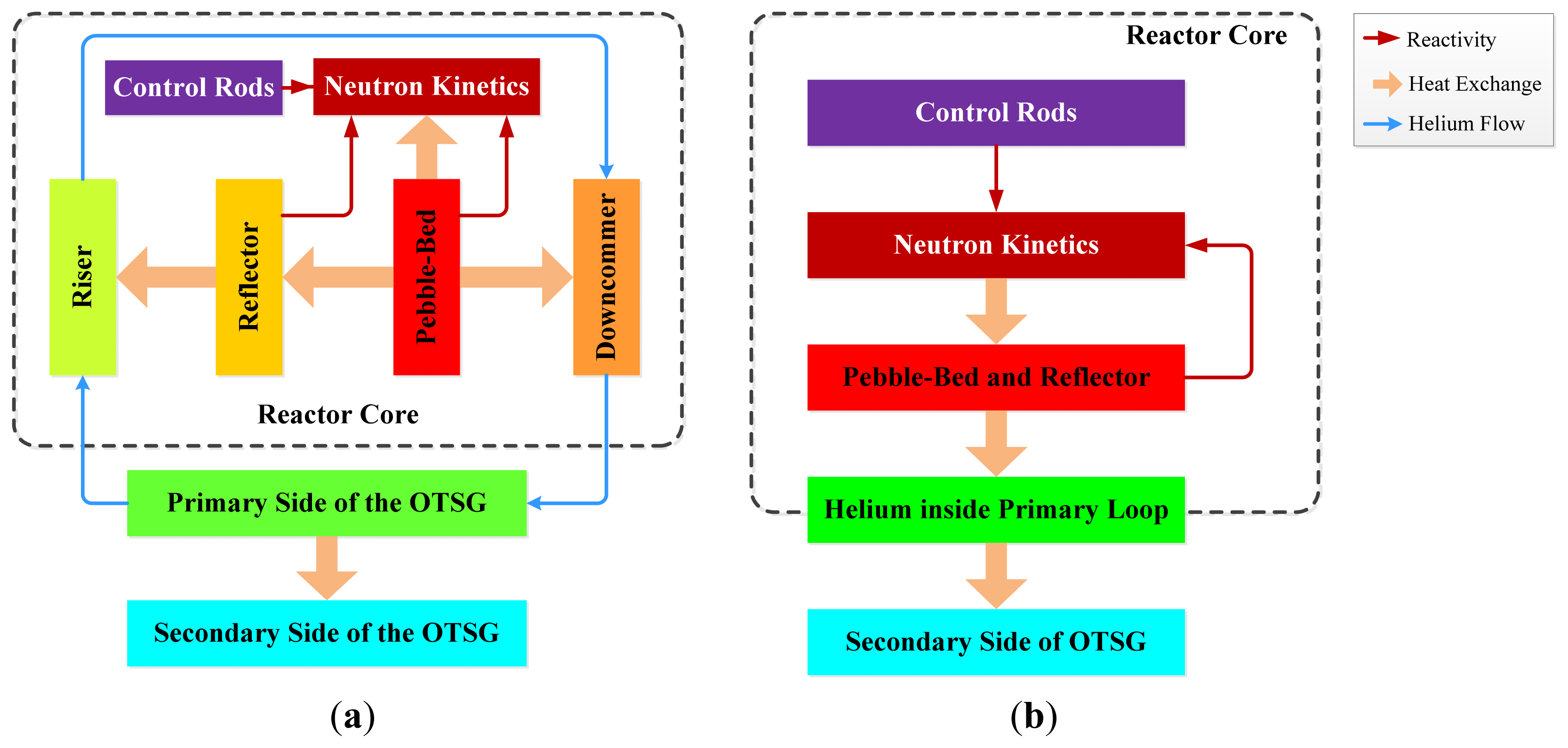
As shown in Figure 1, the MHTGR and OTSG of the NSSS are arranged side by side, and are connected to each other by a horizontal coaxial hot gas duct. The cold helium enters the main blower that is mounted on top of the OTSG, and is pressurized before flowing into the cold gas duct. It enters the channels in the reflector of the core, i.e., the riser from bottom to top, and then passes through the pebble-bed from top to bottom where it is heated to a high temperature. The hot helium leaves the hot gas chamber at the bottom reflector, and then flows into the primary side of the OTSG through the hot gas duct. The primary loop of the NSSS can be nodalized as the elements given in Figure 2a [35], and the control design results in [32–34] were all given based on this nodalization scheme. Since this nodalization scheme reflects too many internal dynamics of the MHTGR, the power-level controllers designed based on this scheme need the values of some unmeasurable internal system variables such as the average temperatures of both the fuel elements and the reflector, which then leads to the demand for designing proper nonlinear observer [32–34]. Moreover, if we regard the pebble bed and the reflector entirely as one node, and also regard all the helium inside the primary-loop as one node, then a simpler nodalization can be formed as illustrated by Figure 2b. Since a simpler nodalization scheme leads to a simpler dynamic model for control design, which then may result in a simpler control system, the dynamic model for control design in this paper is given under this new nodalization scheme.

By adopting the classical point kinetics with one equivalent delayed neutron group and with the temperature reactivity feedback effect determined by the pebble-bed/reflector community, the dynamic model for control design can be written as:

$$\{\begin{array}{l}{\dot{n}}_{\text{r}}=\frac{{\mathrm{\rho }}_{\text{r}}-\mathrm{\beta }}{\mathrm{\Lambda }}{n}_{\text{r}}+\frac{\mathrm{\beta }}{\mathrm{\Lambda }}{c}_{\text{r}}+\frac{{\mathrm{\alpha }}_{\text{R}}}{\mathrm{\Lambda }}{n}_{\text{r}}\left(T_{\text{R}}-T_{\text{R},\text{m}}\right)\hfill \\ {\dot{c}}_{\text{r}}=\mathrm{\lambda }\left(n_{\text{r}}-c_{\text{r}}\right)\hfill \\ {\dot{T}}_{\text{R}}=-\frac{{\mathrm{\Omega }}_{\text{p}}}{{\mathrm{\mu }}_{\text{R}}}\left(T_{\text{R}}-T_{\text{H}}\right)+\frac{P_0}{{\mathrm{\mu }}_{\text{R}}}{n}_{\text{r}}\hfill \\ {\dot{T}}_{\text{H}}=\frac{{\mathrm{\Omega }}_{\text{p}}}{{\mathrm{\mu }}_{\text{H}}}\left(T_{\text{R}}-T_{\text{H}}\right)-\frac{{\mathrm{\Omega }}_{\text{s}}}{{\mathrm{\mu }}_{\text{H}}}\left(T_{\text{H}}-T_{\text{S}}\right)\hfill \\ {\dot{\mathrm{\rho }}}_{\text{r}}=G_{\text{r}}{z}_{\text{r}}\hfill \end{array}$$

(1)

where n_r is the relative neutron power; c_r is the relative concentration of delayed neutron precursor; β is the fraction of delayed fission neutrons; Λ is the effective prompt neutron life time; ρ_r is the reactivity provided by the control rods; λ is the effective radioactive decay constant of the precursor; T_R and α_R is respectively the temperature and reactivity feedback coefficient of the community constituted by both the pebble-bed and reflector; T_R,m is the initial equilibrium value of T_R; P₀ is the rated reactor thermal power; T_H is the average helium temperature of the primary side; T_S is the average coolant temperature of the secondary side of the OTSG; Ω_p is the heat transfer coefficient between the helium and pebble-bed/reflector community; Ω_s is the heat transfer coefficient between the two sides of OTSG; μ_R and μ_H is respectively the total heat capacities of the pebble-bed/reflector community and the helium inside the primary loop; G_r is the total differential reactivity worth of the control rod; and z_r is the rod speed signal. Here, it is worthy to be noted that α_R is guaranteed to be negative by the physical design of the MHTGR.

We define the deviations of the actual values of n_r, c_r, T_R, T_H, T_S and ρ_r from their equilibrium values, i.e., n_r0, c_r0, T_R0, T_H0 and ρ_r0 as:

$$\{\begin{array}{l}\mathrm{\delta }{n}_{\text{r}}=n_{\text{r}}-n_{\text{r}0}\hfill \\ \mathrm{\delta }{c}_{\text{r}}=c_{\text{r}}-c_{\text{r0}}\hfill \\ \mathrm{\delta }{T}_{\text{R}}=T_{\text{R}}-T_{\text{R}0}\hfill \\ \mathrm{\delta }{T}_{\text{H}}=T_{\text{H}}-T_{\text{H}0}\hfill \\ \mathrm{\delta }{T}_{\text{S}}=T_{\text{S}}-T_{\text{S}0}\hfill \\ \mathrm{\delta }{\mathrm{\rho }}_{\text{r}}={\mathrm{\rho }}_{\text{r}}-{\mathrm{\rho }}_{\text{r}0}\hfill \end{array}$$

(2)

Here, δT_S reflects the influence of the secondary to the primary loop, and can be well suppressed by adjusting the feedwater flowrate of the OTSG. Therefore, in this paper, the influence of δT_S is omitted.

Let:

$$\mathit{x}={\left[\begin{array}{cccc}{x}_1& x_2& x_3& x_4\end{array}\right]}^{\text{T}}={\left[\begin{array}{cccc}\mathrm{\delta }{n}_{\text{r}}& \mathrm{\delta }{c}_{\text{r}}& \mathrm{\delta }{T}_{\text{R}}& \mathrm{\delta }{T}_{\text{H}}\end{array}\right]}^{\text{T}}$$

(3)

$$\mathrm{\xi }=\mathrm{\delta }{\mathrm{\rho }}_{\text{r}}$$

(4)

and:

$$u=G_{\text{r}}{z}_{\text{r}}$$

(5)

Here, x is the reactor state-vector of the MHTGR. Then, the nonlinear state-space model for controller design can be written as:

$$\{\begin{array}{l}\dot{\mathit{x}}=\mathit{\text{f}}\left(\mathit{x}\right)+\mathit{g}\left(\mathit{x}\right)\mathrm{\xi }\hfill \\ \dot{\mathrm{\xi }}=u\hfill \\ \mathit{y}=\mathit{h}\left(\mathit{x}\right)\hfill \end{array}$$

(6)

where:

$$\mathit{f}\left(\mathit{x}\right)=\left[\begin{array}{c}-\frac{\mathrm{\beta }}{\mathrm{\Lambda }}\left(x_1-x_2\right)+\frac{{\mathrm{\alpha }}_{\text{R}}}{\mathrm{\Lambda }}\left(n_{\text{r0}}+x_1\right)x_3\\ \mathrm{\lambda }\left(x_1-x_2\right)\\ \frac{P_0}{{\mathrm{\mu }}_{\text{R}}}{x}_1-\frac{{\mathrm{\Omega }}_{\text{p}}}{{\mathrm{\mu }}_{\text{R}}}\left(x_3-x_4\right)\\ \frac{{\mathrm{\Omega }}_{\text{p}}}{{\mathrm{\mu }}_{\text{H}}}\left(x_3-x_4\right)-\frac{{\mathrm{\Omega }}_{\text{s}}}{{\mathrm{\mu }}_{\text{H}}}{x}_4\end{array}\right]$$

(7)

$$\mathit{g}\left(\mathit{x}\right)={\left[\begin{array}{cc}\frac{n_{\text{r0}}+x_1}{\mathrm{\Lambda }}& {\mathit{\text{O}}}_{1\times 3}\end{array}\right]}^{\text{T}}$$

(8)

and:

$$\mathit{h}\left(\mathit{x}\right)={\left[\begin{array}{cc}{x}_1& x_4\end{array}\right]}^{\text{T}}$$

(9)

2.2. Theoretical Problem

Usually, in practical engineering it is nearly impossible to obtain reactor parameters such as Ω_s, μ_R and μ_H accurately. It is necessary to provide acceptable control performance if there exists parameter uncertainty. Thus, the theoretical problem to be solved in the next section is summarized as follows:

Problem

How to design an output-feedback control law of nonlinear system in Equation (6) so that the reactor state are bounded stable, i.e., x ∈ Ξ as t → ∞ when there exists bounded parameter uncertainty? Here, Ξ is a bounded set.

3. Output Feedback Control Design

In this section, we firstly prove that the output feedback power-level control [20] with the simple PD structure can provide globally asymptotic closed-loop stability for MHTGRs. However, since some feedback gains of this PD controller is tightly related with system parameters, an MLP network (MLPN) was utilized to compensate for the influence of system parameter uncertainty. Then, it is proved theoretically that bounded closed-loop stability can be provided with the existence of system parameter uncertainty.

3.1. PD Power-Level Control Design without the Existence of Parameter Uncertainty

The following Theorem 1, which is the first main result of this paper, shows that simple static output-feedback PD power-level control law can guarantee asymptotic closed-loop stability of reactor state-variables in case of no system parameter uncertainty.

Theorem 1

Suppose that there is no system parameter uncertainty. Then, there always exists a PD power-level control law which can provide the asymptotic closed-loop stability for the reactor state of the MHTGR, i.e., x → O as t → ∞.

Proof

Based on the idea of backstepping [13], a virtual control input ξ_r for the following subsystem:

$$\{\begin{array}{l}\dot{\mathit{x}}=\mathit{f}\left(\mathit{x}\right)+\mathit{g}\left(\mathit{x}\right){\mathrm{\xi }}_{\text{r}}\hfill \\ \mathit{\text{y}}=\mathit{h}\left(\mathit{x}\right)\hfill \end{array}$$

(10)

is firstly designed.

From [20], the shifted-ectropy of neutron kinetics is:

$${\mathrm{\zeta }}_{\text{N}}\left(x_1,x_2\right)=n_{\text{r}0}\left\{\mathrm{\Lambda }\left[\left(1+\frac{x_1}{n_{\text{r}0}}\right)-ln\left(1+\frac{x_1}{n_{\text{r}0}}\right)\right]+\frac{\mathrm{\beta }}{\mathrm{\lambda }}\left[\left(1+\frac{x_2}{n_{\text{r}0}}\right)-ln\left(1+\frac{x_2}{n_{\text{r}0}}\right)\right]\right\}$$

(11)

Based on Equation (11), choose the Lyapunov function for the neutron kinetics as:

$$V_{\text{N}}\left(x_1,x_2\right)={\mathrm{\zeta }}_{\text{N}}\left(x_1,x_2\right)+\frac{k_{\text{I}}}{2}{\left[\underset{0}{\overset{t}{\int }}{x}_1\left(s\right)\text{d}s\right]}^2$$

(12)

where the objective of adding the second term of V_N is to minimize the steady error of n_r by feedback control. Then, differentiate V_N along the trajectory given by neutron kinetics, and we have:

$${\dot{V}}_{\text{N}}\left(x_1,x_2\right)=-\frac{\mathrm{\beta }{\left(x_1-x_2\right)}^2}{\left(n_{\text{r0}}+x_1\right)\left(n_{\text{r0}}+x_2\right)}+x_1\left[{\mathrm{\xi }}_{\text{r}}+{\mathrm{\alpha }}_{\text{R}}{x}_3+k_{\text{I}}\underset{0}{\overset{t}{\int }}{x}_1\left(s\right)\text{d}s\right]$$

(13)

Moreover, it is clear that the shifted-ectropy of reactor thermal-hydraulics can be written as:

$${\mathrm{\zeta }}_{\text{T}}\left(x_3,x_4\right)=\frac{1}{2}\left({\mathrm{\mu }}_{\text{R}}{x}_3^2+{\mathrm{\mu }}_{\text{H}}{x}_4^2\right)$$

(14)

Then, based on Equation (14), choose the Lyapunov function for the thermal-hydraulic loop as:

$$V_{\text{T}}\left(x_3,x_4\right)=\left(1-\mathrm{\gamma }\right){\mathrm{\zeta }}_{\text{T}}\left(x_3,x_4\right)+\mathrm{\gamma }{\mathrm{\varsigma }}_{\text{T}}\left(x_3,x_4\right)$$

(15)

where γ is a positive given constant satisfying 0 < γ <1, and:

$${\mathrm{\varsigma }}_{\text{T}}=\frac{1}{2{\mathrm{\mu }}_{\text{R}}}{\left[{\mathrm{\mu }}_{\text{R}}{x}_3+{\mathrm{\mu }}_{\text{H}}{x}_4+{\mathrm{\Omega }}_{\text{S}}\underset{0}{\overset{t}{\int }}{x}_4\left(s\right)\text{d}s\right]}^2$$

(16)

denotes the energy variation of the thermal-hydraulic loops. Then, differentiate Equation (15) along the trajectory given by the reactor thermal-hydraulics:

$$\begin{array}{c}{\dot{V}}_{\text{T}}\left(x_3,x_4\right)=P_0{x}_1{x}_3+\mathrm{\gamma }{P}_0{x}_1\left[\frac{{\mathrm{\mu }}_{\text{H}}}{{\mathrm{\mu }}_{\text{R}}}{x}_4+\frac{{\mathrm{\Omega }}_s}{{\mathrm{\mu }}_{\text{R}}}\underset{0}{\overset{t}{\int }}{x}_4\left(s\right)\text{d}s\right]-\left(1-\mathrm{\gamma }\right)\left(1-\mathrm{\eta }\right)\left[{\mathrm{\Omega }}_{\text{p}}{\left(x_3-x_4\right)}^2+{\mathrm{\Omega }}_s{x}_4^2\right]-\\ \left(1-\mathrm{\gamma }\right)\mathrm{\eta }\left[\left({\mathrm{\Omega }}_{\text{p}}+{\mathrm{\Omega }}_{\text{s}}\right){\left(x_4-\frac{{\mathrm{\Omega }}_{\text{p}}}{{\mathrm{\Omega }}_{\text{p}}+{\mathrm{\Omega }}_{\text{s}}}{x}_3\right)}^2+\frac{{\mathrm{\Omega }}_{\text{p}}{\mathrm{\Omega }}_{\text{s}}}{{\mathrm{\Omega }}_{\text{p}}+{\mathrm{\Omega }}_{\text{s}}}{x}_3^2\right]\end{array}$$

(17)

where η is given positive constant satisfying 0 < η < 1.

Choose the Lyapunov function for subsystem in Equation (10) as:

$$V_1\left(\mathit{x}\right)=V_{\text{N}}\left(x_1,x_2\right)+\frac{q_{\text{R}}}{P_0}{V}_{\text{T}}\left(x_3,x_4\right)$$

(18)

where q_R is a given positive constant; V_N and V_T is determined by Equations (12) and (15), respectively. Then, differentiate Equation (18) along the trajectory given by subsystem dynamics in Equation (10), and we can derive that:

$$\begin{array}{ll}{\dot{V}}_1\left(x\right)\hfill & =-\frac{\mathrm{\beta }{\left(x_1-x_2\right)}^2}{\left(n_{\text{r}0}+x_1\right)\left(n_{\text{r}0}+x_2\right)}-\left(1-\mathrm{\gamma }\right)\left(1-\mathrm{\eta }\right)\frac{q_{\text{R}}}{P_0}\left[{\mathrm{\Omega }}_{\text{p}}{\left(x_3-x_4\right)}^2+{\mathrm{\Omega }}_{\text{s}}{x}_4^2\right]-\hfill \\ \hfill & \left(1-\mathrm{\gamma }\right)\mathrm{\eta }{q}_{\text{R}}\frac{{\mathrm{\Omega }}_{\text{p}}+{\mathrm{\Omega }}_{\text{s}}}{P_0}{\left(x_4-\frac{{\mathrm{\Omega }}_{\text{p}}}{{\mathrm{\Omega }}_{\text{p}}+{\mathrm{\Omega }}_{\text{s}}}{x}_3\right)}^2-\frac{q_{\text{R}}\left(1-\mathrm{\gamma }\right)\mathrm{\eta }{\mathrm{\Omega }}_{\text{p}}{\mathrm{\Omega }}_{\text{s}}}{2P_0\left({\mathrm{\Omega }}_{\text{p}}+{\mathrm{\Omega }}_{\text{s}}\right)}\left\{x_3^2+{\left[x_3-\frac{\left({\mathrm{\Omega }}_{\text{p}}+{\mathrm{\Omega }}_{\text{s}}\right)P_0}{\left(1-\mathrm{\gamma }\right)\mathrm{\eta }{\mathrm{\Omega }}_{\text{p}}{\mathrm{\Omega }}_{\text{s}}}\left(1+\frac{{\mathrm{\alpha }}_{\text{R}}}{q_{\text{R}}}\right)x_1\right]}^2\right\}+\hfill \\ \hfill & x_1\left\{{\mathrm{\xi }}_{\text{r}}+\frac{q_{\text{R}}{P}_0\left({\mathrm{\Omega }}_{\text{P}}+{\mathrm{\Omega }}_{\text{S}}\right)}{2\left(1-\mathrm{\gamma }\right)\mathrm{\eta }{\mathrm{\Omega }}_{\text{P}}{\mathrm{\Omega }}_S}{\left(1+\frac{{\mathrm{\alpha }}_{\text{R}}}{q_{\text{R}}}\right)}^2{x}_1+k_{\text{I}}\underset{0}{\overset{t}{\int }}{x}_1\left(s\right)\text{d}s+\mathrm{\gamma }{q}_{\text{R}}\left[\frac{{\mathrm{\mu }}_{\text{H}}}{{\mathrm{\mu }}_{\text{R}}}{x}_4+\frac{{\mathrm{\Omega }}_{\text{s}}}{{\mathrm{\mu }}_{\text{R}}}\underset{0}{\overset{t}{\int }}{x}_4\left(s\right)\text{d}s\right]\right\}\hfill \end{array}$$

(19)

From Equation (19), it is clear that if we design virtual control ξ_r as:

$${\mathrm{\xi }}_{\text{r}}=-k_{\text{ND}}{x}_1-k_{\text{I}}\underset{0}{\overset{t}{\int }}{x}_1\left(s\right)\text{d}s-\mathrm{\gamma }{q}_{\text{R}}\left[\frac{{\mathrm{\mu }}_{\text{H}}}{{\mathrm{\mu }}_{\text{R}}}{x}_4+\frac{{\mathrm{\Omega }}_{\text{s}}}{{\mathrm{\mu }}_{\text{R}}}\underset{0}{\overset{t}{\int }}{x}_4\left(s\right)\text{d}s\right]$$

(20)

where:

$$k_{\text{ND}}>\frac{q_{\text{R}}{P}_0\left({\mathrm{\Omega }}_{\text{P}}+{\mathrm{\Omega }}_{\text{S}}\right)}{2\left(1-\mathrm{\gamma }\right)\mathrm{\eta }{\mathrm{\Omega }}_{\text{P}}{\mathrm{\Omega }}_{\text{S}}}{\left(1+\frac{{\mathrm{\alpha }}_R}{q_{\text{R}}}\right)}^2$$

(21)

then the closed-loop subsystem constituted by Equations (10) and (20) is asymptotically stable.

Now, we focus on designing the control law for entire system in Equation (6). Choose the Lyapunov function of the entire system as:

$$V_2\left(\mathit{x},e_{\mathrm{\xi }}\right)=V_1\left(\mathit{x}\right)+\frac{e_{\mathrm{\xi }}^2}{2k_{\mathrm{\xi }}}$$

(22)

where k_ξ is a given positive constant, and:

$$e_{\mathrm{\xi }}=\mathrm{\xi }-{\mathrm{\xi }}_{\text{r}}$$

(23)

Differentiate Equation (22) along the trajectory given by entire system dynamics in Equation (6), and we have:

$$\begin{array}{ll}{\dot{V}}_2\left(\mathit{\text{x}},e_{\mathrm{\xi }}\right)\hfill & ={\dot{V}}_1\left(\mathit{\text{x}}\right)+\frac{1}{k_{\mathrm{\xi }}}{e}_{\mathrm{\xi }}{\dot{e}}_{\mathrm{\xi }}\hfill \\ \hfill & =-\frac{\mathrm{\beta }{\left(x_1-x_2\right)}^2}{\left(n_{\text{r0}}+x_1\right)\left(n_{\text{r0}}+x_2\right)}-\left(1-\mathrm{\gamma }\right)\left(1-\mathrm{\eta }\right)\frac{q_{\text{R}}}{P_0}\left[{\mathrm{\Omega }}_{\text{p}}{\left(x_3-x_4\right)}^2+{\mathrm{\Omega }}_{\text{s}}{x}_4^2\right]-\left(1-\mathrm{\gamma }\right)\mathrm{\eta }{q}_{\text{R}}\frac{{\mathrm{\Omega }}_{\text{p}}+{\mathrm{\Omega }}_{\text{s}}}{P_0}{\left(x_4-\frac{{\mathrm{\Omega }}_{\text{p}}}{{\mathrm{\Omega }}_{\text{p}}+{\mathrm{\Omega }}_{\text{s}}}{x}_3\right)}^2-\hfill \\ \hfill & \frac{q_{\text{R}}\left(1-\mathrm{\gamma }\right)\mathrm{\eta }{\mathrm{\Omega }}_{\text{p}}{\mathrm{\Omega }}_{\text{s}}}{2P_0\left({\mathrm{\Omega }}_{\text{p}}+{\mathrm{\Omega }}_{\text{s}}\right)}\left\{x_3^2+{\left[x_3-\frac{\left({\mathrm{\Omega }}_{\text{p}}+{\mathrm{\Omega }}_{\text{s}}\right)P_0}{\left(1-\mathrm{\gamma }\right)\mathrm{\eta }{\mathrm{\Omega }}_{\text{p}}{\mathrm{\Omega }}_{\text{s}}}\left(1+\frac{{\mathrm{\alpha }}_{\text{R}}}{q_{\text{R}}}\right)x_1\right]}^2\right\}-{\stackrel{\sim }{k}}_{\text{ND}}{x}_1^2+x_1{e}_{\mathrm{\xi }}+\frac{1}{k_{\mathrm{\xi }}}{e}_{\mathrm{\xi }}\left(u-{\dot{\mathrm{\xi }}}_{\text{r}}\right)\hfill \end{array}$$

(24)

where:

$${\stackrel{\sim }{k}}_{\text{ND}}=k_{\text{ND}}-\frac{q_{\text{R}}{P}_0\left({\mathrm{\Omega }}_{\text{P}}+{\mathrm{\Omega }}_{\text{S}}\right)}{2\left(1-\mathrm{\gamma }\right)\mathrm{\eta }{\mathrm{\Omega }}_{\text{P}}{\mathrm{\Omega }}_S}{\left(1+\frac{{\mathrm{\alpha }}_{\text{R}}}{q_{\text{R}}}\right)}^2$$

(25)

From Equation (24), if we design feedback control u as:

$$u=-k_{\mathrm{\xi }}{x}_1+{\dot{\mathrm{\xi }}}_{\text{r}}=-\left(k_{\text{NP}}{x}_1+k_{\text{ND}}{\dot{x}}_1+k_{\text{TP}}{x}_4+k_{\text{TD}}{\dot{x}}_4\right)$$

(26)

where:

$$k_{\text{NP}}=k_{\mathrm{\xi }}+k_{\text{I}}$$

(27)

$$k_{\text{TP}}=\mathrm{\gamma }{q}_{\text{R}}\frac{{\mathrm{\Omega }}_{\text{s}}}{{\mathrm{\mu }}_{\text{R}}}$$

(28)

and:

$$k_{\text{TD}}=\mathrm{\gamma }{q}_{\text{R}}\frac{{\mathrm{\mu }}_{\text{H}}}{{\mathrm{\mu }}_{\text{R}}}$$

(29)

then we have:

$$\begin{array}{ll}{\dot{V}}_2\left(\mathit{x},e_{\mathrm{\xi }}\right)\hfill & =-{\stackrel{\sim }{k}}_{\text{ND}}{x}_1^2-\frac{\mathrm{\beta }{\left(x_1-x_2\right)}^2}{\left(n_{\text{r}0}+x_1\right)\left(n_{\text{r}0}+x_2\right)}-\left(1-\mathrm{\gamma }\right)\left(1-\mathrm{\eta }\right)\frac{q_{\text{R}}}{P_0}\left[{\mathrm{\Omega }}_{\text{p}}{\left(x_3-x_4\right)}^2+{\mathrm{\Omega }}_{\text{s}}{x}_4^2\right]-\hfill \\ \hfill & \left(1-\mathrm{\gamma }\right)\mathrm{\eta }{q}_{\text{R}}\frac{{\mathrm{\Omega }}_{\text{p}}+{\mathrm{\Omega }}_{\text{s}}}{P_0}{\left(x_4-\frac{{\mathrm{\Omega }}_p}{{\mathrm{\Omega }}_{\text{p}}+{\mathrm{\Omega }}_{\text{s}}}{x}_3\right)}^2-\frac{q_{\text{R}}\left(1-\mathrm{\gamma }\right)\mathrm{\eta }{\mathrm{\Omega }}_{\text{p}}{\mathrm{\Omega }}_{\text{s}}}{2P_0\left({\mathrm{\Omega }}_{\text{p}}+{\mathrm{\Omega }}_{\text{s}}\right)}\left\{x_3^2+{\left[x_3-\frac{\left({\mathrm{\Omega }}_{\text{p}}+{\mathrm{\Omega }}_{\text{s}}\right)P_0}{\left(1-\mathrm{\gamma }\right)\mathrm{\eta }{\mathrm{\Omega }}_{\text{p}}{\mathrm{\Omega }}_{\text{s}}}\left(1+\frac{{\mathrm{\alpha }}_{\text{R}}}{q_{\text{R}}}\right)x_1\right]}^2\right\}\hfill \end{array}$$

(30)

Based on Equation (30), it is clear that there always exists a PD power-level controller in Equation (26), so that reactor state x of MHTGR dynamics in Equation (6) is asymptotically stable. This completes the proof of this theorem.

Remark 1

From Equations (12) and (27), it is clear that we can suppressing the steady error of nuclear power through enlarging the proportional feedback gain k_NP corresponding to δn_r. Moreover, from Equation (18), we can also strengthen the dynamic performance of the thermal-hydraulic loop through enlarging q_R, which certainly leads to larger values of feedback gains k_ND, k_TP and k_TD.

Remark 2

Since positive constants γ and η can be arbitrarily chosen between 0 and 1, inequality in Equation (21) is easy to satisfy by choosing γ to be close enough to 1 and η to be close enough to 0. However, larger γ also leads to larger k_TP and k_TD.

3.2. MLP-Compensated PD Power-Level Control Design with the Existence of Parameter Uncertainty

Based upon the analysis given in Remarks 1 and 2, although inequality in Equation (21) is easy to be satisfied. There is still tight relationship between feedback gains k_TP and k_TD and system parameters Ω_s, μ_R and μ_H. Applying PD control law in Equation (26) requires the precise values of parameters Ω_s, μ_R and μ_H which are all very difficult to obtain accurately. Therefore, there must exists uncertainty in of parameters Ω_s, μ_R and μ_H, and the practically implemented of PD power-level controller may be:

$$u_{\text{A}}=-\left(k_{\text{NP}}{x}_1+k_{\text{ND}}{\dot{x}}_1+k_{\text{TPA}}{x}_4+k_{\text{TDA}}{\dot{x}}_4\right)$$

(31)

where feedback gains k_NP and k_ND satisfies Equations (27) and (21), respectively; and both feedback gains k_TPA and k_TDA are positive scalars chosen experientially. Then, define:

$$u_{\text{e}}=u_{\text{A}}-u=-\left(k_{\text{TPe}}{x}_4+k_{\text{TDe}}{\dot{x}}_4\right)$$

(32)

where u is defined in Equation (26), and:

$$\{\begin{array}{l}{k}_{\text{TPe}}=k_{\text{TPA}}-k_{\text{TP}}\hfill \\ k_{\text{TDe}}=k_{\text{TDA}}-k_{\text{TD}}\hfill \end{array}$$

(33)

It is clear that the uncertainty of system parameters Ω_s, μ_R and μ_H results in nonzero k_TPe or k_TDe, which then leads to the existence of nonzero u_e determined by Equation (32). In practical engineering, we should design another term v in the power-level controller to compensate the influence of u_e so that the closed-loop system is bounded stable.

Due to the strong capability of MLPN in function approximation, an MLPN is utilized to build the compensating term v in this section. Before giving the design result, we firstly introduce the MLPN.

The mutli-input-single-output MLPN can be expressed as [36]:

$$G_{\text{MLP}}\left(\mathit{z}\right)={\mathit{\text{W}}}^{\text{T}}\mathit{\text{S}}({\mathit{\text{V}}}^{\text{T}}\overline{z})$$

(34)

where z ∈ Rⁿ is the input vector, V ∈ R^(n+1)×l and W ∈ R^l is respectively the first-to-second layer and second-to-third layer interconnection matrices, l is the number of neurons in the hidden layer, n is the number of input:

$$\overline{z}={\left[\begin{array}{cc}{z}^{\text{T}}& 1\end{array}\right]}^{\text{T}}$$

(35)

and:

$$\mathit{\text{S}}({\mathit{\text{V}}}^{\text{T}}\overline{z})={\left[\begin{array}{cccc}s({\mathit{v}}_1^{\text{T}}\overline{\mathit{z}})& s({\mathit{v}}_2^{\text{T}}\overline{\mathit{z}})& \dots & s({\mathit{v}}_l^{\text{T}}\overline{\mathit{z}})\end{array}\right]}^{\text{T}}$$

(36)

here, vector v_i (i = 1, …, l) is the ith column of interconnection matrix V; and activation function s is chosen as the hyperbolic tangent function, i.e.,

$$s\left(t\right)=\frac{e^t-e^{-t}}{e^t+e^{-t}},\forall t\in \text{R}$$

(37)

in this paper.

It has been proved in [37] that if the node number l of the hidden layer is large enough, then MLPN in Equation (34) can approximate an arbitrarily given continuous function h: Rⁿ → R to arbitrary accuracy on a compact set, i.e.,

$$h\left(\mathit{\text{z}}\right)={\mathit{\text{G}}}_{\text{MLP}}\left(\mathit{z}\right)+d_{\text{e}},\forall \mathit{z}\in {\mathrm{\Pi }}_z\subset {\text{R}}^n$$

(38)

here, d_e is the approximation error, and Π_z is a compact set on which W and V are bounded, i.e.,

$${\Vert \mathit{W}\Vert }_2\le w_{\text{m}}$$

(39)

and:

$${\Vert \mathit{V}\Vert }_{\text{F}}\le v_{\text{m}}$$

(40)

where:

$${\Vert \mathit{\text{V}}\Vert }_{\text{F}}=\sqrt{\text{tr}({\mathit{\text{V}}}^{\text{T}}\mathit{\text{V}})}$$

(41)

In general, the ideal weights W and V are unknown and need to be estimated in control design. Let Ŵ and V̂ be the estimates of W and V respectively, and also define the weight estimation error as:

$$\{\begin{array}{l}\stackrel{\sim }{\mathit{\text{W}}}=\hat{\mathit{W}}-\mathit{W}\hfill \\ \stackrel{\sim }{\mathit{\text{V}}}=\hat{\mathit{V}}-\mathit{V}\hfill \end{array}$$

(42)

Now, an important property of the estimation error of MLPN in Equation (34) is introduced as the following lemma.

Lemma 1 [38]

The corresponding approximation error χ of MLPN in Equation (34) can be expressed as:

$$\chi ={\hat{G}}_{\text{MLP}}\left(\text{z}\right)-G_{\text{MLP}}\left(\text{z}\right)={\stackrel{\sim }{\mathit{W}}}^{\text{T}}\left(\hat{\mathit{S}}-{\hat{\mathit{S}}}^{\prime }{\hat{\mathit{V}}}^{\text{T}}\overline{\mathit{z}}\right)+{\hat{\mathit{W}}}^{\text{T}}{\hat{\mathit{S}}}^{\prime }{\stackrel{\sim }{\mathit{V}}}^{\text{T}}\overline{\mathit{z}}+d_{\text{u}}$$

(43)

where:

$${\hat{G}}_{\text{MLP}}\left(\mathit{\text{z}}\right)={\hat{\mathit{W}}}^{\text{T}}\mathit{\text{S}}\left({\hat{\mathit{V}}}^{\text{T}}\overline{\mathit{z}}\right)$$

(44)

$$\widehat{\mathit{\text{S}}}=\mathit{S}\left({\hat{\mathit{V}}}^{\text{T}}\overline{\mathit{z}}\right)$$

(45)

$${\hat{\mathit{S}}}^{\prime }=\text{diag}\left({\left[\begin{array}{cccc}{\hat{s}}_1^{\prime }& {\hat{s}}_2^{\prime }& \cdots & {\hat{s}}_l^{\prime }\end{array}\right]}^{\text{T}}\right)$$

(46)

$${{{\hat{s}}^{\prime }}_i=s^{\prime }({\hat{v}}_i^{\text{T}}z)=\frac{\text{d}s\left(t\right)}{\text{d}t}|}_{t={\hat{v}}_i^{\text{T}}z}\left(i=1,2,\dots ,l\right)$$

(47)

v̂_i is the ith column of interconnection matrix V̂. Moreover, the residual term d_u is bounded by:

$$d_{\text{u}}\le {\Vert \mathit{V}\Vert }_{\text{F}}{\Vert \overline{\mathit{z}}{\widehat{\mathit{\text{W}}}}^{\text{T}}{\hat{\mathit{S}}}^{\prime }\Vert }_{\text{F}}+{\Vert \mathit{\text{W}}\Vert }_2{\Vert {\hat{\mathit{S}}}^{\prime }{\hat{\mathit{V}}}^{\text{T}}\overline{\mathit{z}}\Vert }_2+{\Vert \mathit{W}\Vert }_1$$

(48)

where:

$${\Vert \mathit{\text{W}}\Vert }_1=\sum _{i=1}^l\left|w_i\right|$$

(49)

and w_i is the ith element of network weighting W.

Remark 3

From Equation (34), it is clear that the MLPN is essentially a nonlinearly parameterized function approximator, i.e., the hidden layer weight V appears in a nonlinear fashion. Thus, when applying Ĝ_MLP for solving approximation problem, it is highly desirable to have a linearly parameter-ization of approximation error χ. The value of Lemma 1 is giving a linearly parameterized form of χ in terms of W̃ and Ṽ, which is very useful in designing learning algorithms of the MLPN weighting matrices. Based upon the above introduction, we summarize the second main result of this paper in the following Theorem 2, which guarantees reactor state x to be bounded closed-loop stable with the existence of uncertainty of parameters Ω_s, μ_R and μ_H.

Theorem 2

Consider the existence of uncertainty in parameters Ω_s, μ_R and μ_H. Define:

$$\mathrm{\theta }=k_{\text{TDe}}{x}_4+k_{\text{TPe}}\underset{0}{\overset{t}{\int }}{x}_4\left(s\right)\text{d}s$$

(50)

and suppose that uncertainty θ can be approximated by a MLPN, i.e.,

$$\mathrm{\theta }={\mathit{\text{W}}}^{\text{T}}\mathit{S}({\mathit{V}}^{\text{T}}\overline{\mathit{z}})+d_{\text{e}}$$

(51)

where z̄ and S satisfy Equations (35) and (36), respectively, approximation error d_e is bounded, and both weighting vector W and weighting matrix V are bounded and constant, i.e., Ẇ ≡ Ȯ and V̇ ≡ O. Design the control input as:

$$u=u_{\text{A}}+v$$

(52)

where:

$$v=\frac{\text{d}}{\text{d}t}\left[G_{\text{MLP}}\left(\mathit{z}\right)\right]=\frac{\text{d}}{\text{d}t}\left[{\hat{\mathit{W}}}^{\text{T}}\mathit{S}\left({\hat{\mathit{V}}}^{\text{T}}\overline{\mathit{z}}\right)\right]$$

(53)

$$\mathit{z}=\mathit{\text{U}}\overline{\mathit{y}}$$

(54)

$$\overline{\mathit{y}}={\left[\begin{array}{cccccc}{x}_1& \underset{0}{\overset{t}{\int }}{x}_1\left(s\right)\text{d}s& {\dot{x}}_1& x_4& \underset{0}{\overset{t}{\int }}{x}_4\left(s\right)\text{d}s& {\dot{x}}_4\end{array}\right]}^{\text{T}}$$

(55)

u_A, z̄ and S satisfy Equations (31), (35) and (36), respectively; and U ∈ R^6×6 is a given diagonally positive-definite matrix. Here, the learning algorithms of weighting matrices Ŵ and V̂ in Equation (53) are designed respectively as:

$$\dot{\hat{\mathit{W}}}=-{\mathit{\Gamma }}_{\text{W}}\left[\left(\hat{\mathit{S}}-{\hat{\mathit{S}}}^{\prime }{\hat{\mathit{V}}}^{\text{T}}\overline{\mathit{z}}\right)x_1+{\delta }_{\text{W}}\hat{\mathit{W}}\right]$$

(56)

$$\dot{\hat{\mathit{V}}}=-{\mathit{\Gamma }}_{\text{V}}\left(\overline{\mathit{z}}{\hat{\mathit{W}}}^{\text{T}}{\hat{\mathit{S}}}^{\prime }{x}_1+{\delta }_{\text{V}}\hat{\mathit{V}}\right)$$

(57)

where both δ_W and δ_V are given positive scalars, and both Γ_W and Γ_V are given positive-definite matrices. Then, the power-level control law constituted by Equations (31), (52), (53), (56) and (57) guarantees closed-loop bounded stability of reactor state x if:

$$k_{\text{ND}}-\frac{q_{\text{R}}{P}_0\left({\mathrm{\Omega }}_{\text{P}}+{\mathrm{\Omega }}_{\text{S}}\right)}{2\left(1-\mathrm{\gamma }\right)\mathrm{\eta }{\mathrm{\Omega }}_{\text{P}}{\mathrm{\Omega }}_S}{\left(1+\frac{{\mathrm{\alpha }}_{\text{R}}}{q_{\text{R}}}\right)}^2-\frac{\epsilon }{2}>0$$

(58)

where ε is an arbitrarily given positive scalar.

Proof

Similarly to the poof of Theorem 1, we also study firstly the stabilization of subsystem in Equation (10) with the existence of system parameter uncertainty. Based on the idea of incorporating MLPN to compensate the parameter uncertainty, we design virtual control ξ_r of subsystem in Equation (10) as:

$${\mathrm{\xi }}_{\text{r}}={\mathrm{\xi }}_{\text{rA}}+{\mathrm{\xi }}_{\text{rC}}$$

(59)

where:

$${\mathrm{\xi }}_{\text{rA}}=-\left[k_{\text{ND}}{x}_1+k_{\text{I}}\underset{0}{\overset{t}{\int }}{x}_1\left(s\right)\text{d}s+k_{\text{TDA}}{x}_4+k_{\text{TPA}}\underset{0}{\overset{t}{\int }}{x}_4\left(s\right)\text{d}s\right]$$

(60)

$${\mathrm{\xi }}_{\text{rC}}={\hat{\mathit{W}}}^{\text{T}}\mathit{\text{S}}\left({\hat{\mathit{V}}}^{\text{T}}\overline{\mathit{z}}\right)$$

(61)

z̄ and S satisfies Equations (35) and (36), respectively.

Moreover, choose the Lyapunov function of subsystem in Equation (10) as:

$$V_3\left(\text{x},\stackrel{\sim }{\mathit{W}},\stackrel{\sim }{\mathit{V}}\right)=V_1\left(x\right)+\frac{1}{2}{\stackrel{\sim }{\mathit{W}}}^{\text{T}}{\mathrm{\Gamma }}_{\text{W}}^{-1}\stackrel{\sim }{\mathit{W}}+\frac{1}{2}\text{tr}\left({\stackrel{\sim }{\mathit{V}}}^{\text{T}}{\mathrm{\Gamma }}_{\text{V}}^{-1}\stackrel{\sim }{\mathit{V}}\right)$$

(62)

Differentiate V₃ given by Equation (62) along the trajectory determined by subsystem dynamics in Equation (10) and control input in Equation (59), and we can derive that:

$$\begin{array}{ll}{\dot{V}}_3(\mathit{x},\stackrel{\sim }{\mathit{\text{W}}},\stackrel{\sim }{\mathit{V}})\hfill & ={\dot{V}}_1\left(\mathit{x}\right)+{\stackrel{\sim }{\mathit{W}}}^T{\mathrm{\Gamma }}_{\text{W}}^{-1}\dot{\stackrel{\sim }{\mathit{W}}}+\text{tr}\left({\stackrel{\sim }{\mathit{V}}}^T{\mathrm{\Gamma }}_{\text{V}}^{-1}\dot{\stackrel{\sim }{\mathit{V}}}\right)\hfill \\ \hfill & =-\frac{\mathrm{\beta }{\left(x_1-x_2\right)}^2}{\left(n_{\text{r}0}+x_1\right)\left(n_{\text{r}0}+x_2\right)}-\left(1-\mathrm{\gamma }\right)\left(1-\mathrm{\eta }\right)\frac{q_{\text{R}}}{P_0}\left[{\mathrm{\Omega }}_{\text{p}}{\left(x_3-x_4\right)}^2+{\mathrm{\Omega }}_{\text{s}}{x}_4^2\right]-\left(1-\mathrm{\gamma }\right)\mathrm{\eta }{q}_{\text{R}}\frac{{\mathrm{\Omega }}_{\text{p}}+{\mathrm{\Omega }}_{\text{s}}}{P_0}{\left(x_4-\frac{{\mathrm{\Omega }}_{\text{p}}}{{\mathrm{\Omega }}_{\text{p}}+{\mathrm{\Omega }}_{\text{s}}}{x}_3\right)}^2-\hfill \\ \hfill & \frac{q_{\text{R}}\left(1-\mathrm{\gamma }\right)\mathrm{\eta }{\mathrm{\Omega }}_{\text{p}}{\mathrm{\Omega }}_{\text{s}}}{2P_0\left({\mathrm{\Omega }}_{\text{p}}+{\mathrm{\Omega }}_{\text{s}}\right)}\left\{x_3^2+{\left[x_3-\frac{\left({\mathrm{\Omega }}_{\text{p}}+{\mathrm{\Omega }}_{\text{s}}\right)P_0}{\left(1-\mathrm{\gamma }\right)\mathrm{\eta }{\mathrm{\Omega }}_{\text{p}}{\mathrm{\Omega }}_{\text{s}}}\left(1+\frac{{\mathrm{\alpha }}_{\text{R}}}{q_{\text{R}}}\right)x_1\right]}^2\right\}-{\stackrel{\sim }{k}}_{\text{ND}}{x}_1^2+x_1\left[{\hat{\mathit{W}}}^{\text{T}}\mathit{\text{S}}\left({\hat{\mathit{V}}}^{\text{T}}\overline{\mathit{z}}\right)-{\mathit{W}}^{\text{T}}\mathit{\text{S}}({\mathit{V}}^{\text{T}}\overline{\mathit{z}})-d_{\text{e}}\right]+\hfill \\ \hfill & {\stackrel{\sim }{\mathit{W}}}^{\text{T}}{\mathrm{\Gamma }}_{\text{W}}^{-1}\dot{\stackrel{\sim }{\mathit{W}}}+\text{tr}\left({\stackrel{\sim }{\mathit{V}}}^T{\mathrm{\Gamma }}_{\text{V}}^{-1}\dot{\stackrel{\sim }{\mathit{V}}}\right)\hfill \end{array}$$

(63)

Based on Lemma 1, it is easy to see that:

$${\widehat{\mathit{\text{W}}}}^{\text{T}}\mathit{\text{S}}\left({\widehat{\mathit{\text{V}}}}^{\text{T}}\overline{\mathit{z}}\right)-{\mathit{W}}^{\text{T}}\mathit{\text{S}}({\mathit{V}}^{\text{T}}\overline{\mathit{z}})-d_{\text{e}}={\stackrel{\sim }{\mathit{W}}}^{\text{T}}\left(\hat{\mathit{S}}-{\hat{\mathit{S}}}^{\prime }{\hat{\mathit{V}}}^{\text{T}}\overline{\mathit{z}}\right)+\text{tr}\left({\stackrel{\sim }{\mathit{V}}}^{\text{T}}\overline{\mathit{z}}{\hat{\mathit{W}}}^{\text{T}}{\hat{\mathit{S}}}^{\prime }\right)+d$$

(64)

where:

$$d=d_{\text{u}}-d_{\text{e}}$$

(64)

is bounded.

Substituting Equation (64) into Equation (63), we have:

$$\begin{array}{ll}{\dot{V}}_3\left(\mathit{x},\stackrel{\sim }{\mathit{W}},\stackrel{\sim }{\mathit{V}}\right)\hfill & =-\frac{\mathrm{\beta }{\left(x_1-x_2\right)}^2}{\left(n_{\text{r0}}+x_1\right)\left(n_{\text{r0}}+x_2\right)}-\left(1-\mathrm{\gamma }\right)\left(1-\mathrm{\eta }\right)\frac{q_{\text{R}}}{P_0}\left[{\mathrm{\Omega }}_{\text{p}}{\left(x_3-x_4\right)}^2+{\mathrm{\Omega }}_{\text{s}}{x}_4^2\right]-\left(1-\mathrm{\gamma }\right)\mathrm{\eta }{q}_{\text{R}}\frac{{\mathrm{\Omega }}_{\text{p}}+{\mathrm{\Omega }}_{\text{s}}}{P_0}{\left(x_4-\frac{{\mathrm{\Omega }}_{\text{p}}}{{\mathrm{\Omega }}_{\text{p}}+{\mathrm{\Omega }}_{\text{s}}}{x}_3\right)}^2-\hfill \\ \hfill & {\stackrel{\sim }{k}}_{\text{ND}}{x}_1^2-\frac{q_{\text{R}}\left(1-\mathrm{\gamma }\right){\mathrm{\eta }\mathrm{\Omega }}_{\text{p}}{\mathrm{\Omega }}_{\text{s}}}{2P_0\left({\mathrm{\Omega }}_{\text{p}}+{\mathrm{\Omega }}_{\text{s}}\right)}\left\{x_3^2+{\left[x_3-\frac{\left({\mathrm{\Omega }}_{\text{p}}+{\mathrm{\Omega }}_{\text{s}}\right)P_0}{\left(1-\mathrm{\gamma }\right){\mathrm{\eta }\mathrm{\Omega }}_{\text{p}}{\mathrm{\Omega }}_{\text{s}}}\left(1+\frac{{\mathrm{\alpha }}_{\text{R}}}{q_{\text{R}}}\right)x_1\right]}^2\right\}+x_{1}d+{\stackrel{\sim }{\mathit{W}}}^{\text{T}}\left[\left(\hat{\mathit{S}}-{\hat{\mathit{S}}}^{\prime }{\hat{\mathit{V}}}^{\text{T}}\overline{\mathit{z}}\right)x_1+{\mathrm{\Gamma }}_{\text{W}}^{-1}\dot{\stackrel{\sim }{\mathit{W}}}\right]+\hfill \\ \hfill & \text{tr}\left({\stackrel{\sim }{\mathit{V}}}^{\text{T}}\overline{\mathit{z}}{x}_1{\hat{\mathit{W}}}^{\text{T}}{\hat{\mathit{S}}}^{\prime }+{\mathrm{\Gamma }}_{\text{V}}^{-1}\dot{\stackrel{\sim }{\mathit{V}}}\right)\hfill \end{array}$$

(66)

From the assumption Ẇ ≡ O and V̇ ≡ O, and by choosing the learning algorithms of weights Ŵ and V̂ as Equations (56) and (57), we have:

$$\begin{array}{c}{\dot{\mathit{\text{V}}}}_3\le -\frac{\mathrm{\beta }{\left(x_1-x_2\right)}^2}{\left(n_{\text{r}0}+x_1\right)\left(n_{\text{r}0}+x_2\right)}-\left(1-\mathrm{\gamma }\right)\left(1-\mathrm{\eta }\right)\frac{q_{\text{R}}}{P_0}\left[{\mathrm{\Omega }}_{\text{p}}{\left(x_3-x_4\right)}^2+{\mathrm{\Omega }}_{\text{s}}{x}_4^2\right]-\left(1-\mathrm{\gamma }\right)\mathrm{\eta }{q}_{\text{R}}\frac{{\mathrm{\Omega }}_{\text{p}}+{\mathrm{\Omega }}_{\text{s}}}{P_0}{\left(x_4-\frac{{\mathrm{\Omega }}_{\text{p}}}{{\mathrm{\Omega }}_{\text{p}}+{\mathrm{\Omega }}_{\text{s}}}{x}_3\right)}^2-{\overline{k}}_{\text{ND}}{x}_1^2-\\ \frac{q_{\text{R}}\left(1-\mathrm{\gamma }\right)\mathrm{\eta }{\mathrm{\Omega }}_{\text{p}}{\mathrm{\Omega }}_{\text{s}}}{2P_0\left({\mathrm{\Omega }}_{\text{p}}+{\mathrm{\Omega }}_{\text{s}}\right)}\left\{x_3^2+{\left[x_3-\frac{\left({\mathrm{\Omega }}_{\text{p}}+{\mathrm{\Omega }}_{\text{s}}\right)P_0}{\left(1-\mathrm{\gamma }\right)\mathrm{\eta }{\mathrm{\Omega }}_{\text{p}}{\mathrm{\Omega }}_{\text{s}}}\left(1+\frac{{\mathrm{\alpha }}_{\text{R}}}{q_{\text{R}}}\right)x_1\right]}^2\right\}-\frac{{\mathrm{\delta }}_{\text{W}}}{2}{\Vert \stackrel{\sim }{\mathit{\text{W}}}\Vert }_2^2-\frac{{\mathrm{\delta }}_{\text{V}}}{2}{\Vert \stackrel{\sim }{\mathit{V}}\Vert }_{\text{F}}^2+\frac{d^2}{2\epsilon }+\frac{{\mathrm{\delta }}_{\text{W}}}{2}{\Vert \mathit{W}\Vert }_2^2+\frac{{\mathrm{\delta }}_{\text{V}}}{2}{\Vert \mathit{V}\Vert }_F^2\end{array}$$

(67)

where:

$${\overline{k}}_{\text{ND}}={\stackrel{\sim }{k}}_{\text{ND}}-\frac{\epsilon }{2}=k_{\text{ND}}-\frac{q_{\text{R}}{P}_0\left({\mathrm{\Omega }}_P+{\mathrm{\Omega }}_{\text{S}}\right)}{2\left(1-\mathrm{\gamma }\right)\mathrm{\eta }{\mathrm{\Omega }}_{\text{P}}{\mathrm{\Omega }}_S}{\left(1+\frac{{\mathrm{\alpha }}_{\text{R}}}{q_{\text{R}}}\right)}^2-\frac{\epsilon }{2}$$

(68)

Now, we focus on the stabilization of entire system in Equation (6). Choose the corresponding Lyapunov function as:

$$V_4\left(\mathit{\text{x}},\stackrel{\sim }{\mathit{W}},\stackrel{\sim }{\mathit{V}},e_{\mathrm{\xi }}\right)=V_3(\mathit{\text{x}},\stackrel{\sim }{\mathit{W}},\stackrel{\sim }{\mathit{V}})+\frac{e_{\mathrm{\xi }}^2}{2k_{\mathrm{\xi }}}$$

(69)

and design control input as:

$$u=-k_{\mathrm{\xi }}{x}_1+{\dot{\mathrm{\xi }}}_{\text{r}}=u_{\text{A}}+{\dot{\mathrm{\xi }}}_{\text{rC}}$$

(70)

where ξ_r, u_A and ξ_rC is given by Equations (59), (31) and (61), respectively. Then, differentiate V₄ along the trajectory given by system dynamics in Equation (6) and control input Equation (70):

$$\begin{array}{ll}{\dot{\mathit{\text{V}}}}_4\hfill & ={\dot{V}}_3+\frac{1}{k_{\mathrm{\xi }}}{e}_{\mathrm{\xi }}\left(u-{\dot{\mathrm{\xi }}}_{\text{r}}\right)\hfill \\ \hfill & \le -\frac{\mathrm{\beta }{\left(x_1-x_2\right)}^2}{\left(n_{\text{r}0}+x_1\right)\left(n_{\text{r}0}+x_2\right)}-\left(1-\mathrm{\gamma }\right)\left(1-\mathrm{\eta }\right)\frac{q_{\text{R}}}{P_0}\left[{\mathrm{\Omega }}_{\text{p}}{\left(x_3-x_4\right)}^2+{\mathrm{\Omega }}_{\text{s}}{x}_4^2\right]-\left(1-\mathrm{\gamma }\right)\mathrm{\eta }{q}_{\text{R}}\frac{{\mathrm{\Omega }}_{\text{p}}+{\mathrm{\Omega }}_{\text{s}}}{P_0}{\left(x_4-\frac{{\mathrm{\Omega }}_{\text{p}}}{{\mathrm{\Omega }}_{\text{p}}+{\mathrm{\Omega }}_{\text{s}}}{x}_3\right)}^2-\hfill \\ \hfill & {\overline{k}}_{\text{ND}}{x}_1^2-\frac{q_{\text{R}}\left(1-\mathrm{\gamma }\right)\mathrm{\eta }{\mathrm{\Omega }}_{\text{p}}{\mathrm{\Omega }}_{\text{s}}}{2P_0\left({\mathrm{\Omega }}_{\text{p}}+{\mathrm{\Omega }}_{\text{s}}\right)}\left\{x_3^2+{\left[x_3-\frac{\left({\mathrm{\Omega }}_{\text{p}}+{\mathrm{\Omega }}_{\text{s}}\right)P_0}{\left(1-\mathrm{\gamma }\right)\mathrm{\eta }{\mathrm{\Omega }}_{\text{p}}{\mathrm{\Omega }}_{\text{s}}}\left(1+\frac{{\mathrm{\alpha }}_{\text{R}}}{q_{\text{R}}}\right)x_1\right]}^2\right\}-\frac{{\mathrm{\delta }}_{\text{W}}}{2}{\Vert \stackrel{\sim }{\mathit{\text{W}}}\Vert }_2^2-\frac{{\mathrm{\delta }}_{\text{V}}}{2}{\Vert \stackrel{\sim }{\mathit{V}}\Vert }_{\text{F}}^2+\frac{d^2}{2\mathit{\epsilon }}+\frac{{\mathrm{\delta }}_{\text{W}}}{2}{\Vert \mathit{W}\Vert }_2^2+\frac{{\mathrm{\delta }}_{\text{V}}}{2}{\Vert \mathit{V}\Vert }_{\text{F}}^2\hfill \end{array}$$

(71)

From the boundness of d, W and V and inequalities in Equations (58) and (71), reactor state x and weight estimation error W̃ and Ṽ converges to bounded set Ξ determined by:

$$\Xi =\left\{\begin{array}{cc}\mathit{x},\stackrel{\sim }{\mathit{W}},\stackrel{\sim }{\mathit{V}}|& \Psi \left(x\right)+\frac{{\mathrm{\delta }}_{\text{W}}}{2}{\Vert \stackrel{\sim }{\mathit{W}}\Vert }_2^2+\frac{{\mathrm{\delta }}_{\text{V}}}{2}{\Vert \stackrel{\sim }{\mathit{V}}\Vert }_{\text{F}}^2\le \frac{d^2}{2\mathit{\epsilon }}+\frac{{\mathrm{\delta }}_{\text{W}}}{2}{\Vert \mathit{W}\Vert }_2^2+\frac{{\mathrm{\delta }}_{\text{V}}}{2}{\Vert \mathit{V}\Vert }_{\text{F}}^2\end{array}\right\}$$

(72)

where:

$$\begin{array}{ll}\Psi \left(x\right)\hfill & ={\overline{k}}_{\text{ND}}{x}_1^2+\frac{\mathrm{\beta }{\left(x_1-x_2\right)}^2}{\left(n_{\text{r}0}+x_1\right)\left(n_{\text{r}0}+x_2\right)}+\left(1-\mathrm{\gamma }\right)\left(1-\mathrm{\eta }\right)\frac{q_{\text{R}}}{P_0}\left[{\mathrm{\Omega }}_{\text{p}}{\left(x_3-x_4\right)}^2+{\mathrm{\Omega }}_{\text{s}}{x}_4^2\right]+\hfill \\ \hfill & \left(1-\mathrm{\gamma }\right)\mathrm{\eta }{q}_{\text{R}}\frac{{\mathrm{\Omega }}_{\text{p}}+{\mathrm{\Omega }}_{\text{s}}}{P_0}{\left(x_4-\frac{{\mathrm{\Omega }}_{\text{p}}}{{\mathrm{\Omega }}_{\text{p}}+{\mathrm{\Omega }}_{\text{s}}}{x}_3\right)}^2+\frac{q_{\text{R}}\left(1-\mathrm{\gamma }\right)\mathrm{\eta }{\mathrm{\Omega }}_{\text{p}}{\mathrm{\Omega }}_{\text{s}}}{2P_0\left({\mathrm{\Omega }}_{\text{p}}+{\mathrm{\Omega }}_{\text{s}}\right)}\left\{x_3^2+{\left[x_3-\frac{\left({\mathrm{\Omega }}_{\text{p}}+{\mathrm{\Omega }}_{\text{s}}\right)P_0}{\left(1-\mathrm{\gamma }\right)\mathrm{\eta }{\mathrm{\Omega }}_{\text{p}}{\mathrm{\Omega }}_{\text{s}}}\left(1+\frac{{\mathrm{\alpha }}_{\text{R}}}{q_{\text{R}}}\right)x_1\right]}^2\right\}\hfill \end{array}$$

(73)

Therefore, from Equations (71) and (72), it is clear that reactor state x is closed-loop bounded stable, which completes the proof of Theorem 2 and solves Problem raised in Section 2.2.

Remark 4

The basic idea of Theorem 2 is incorporating MLPN to compensate the uncertainty in parameters Ω_s, μ_R and μ_H. Due to the fact the approximation error of MLPN is bounded, we cannot guarantee asymptotic closed-loop stability anymore. Instead, bounded closed-loop stability of reactor state x can be provided. However, the bounded stability is enough in practical engineering. Thus, we can easily see that there exists a tradeoff between uncertainty compensation and closed-loop stability.

Remark 5

The novel MLP-compensated PD control for power-level regulation of the MHTGRs presented in this paper can be summarized as:

$$\{\begin{array}{l}u=u_{\text{A}}+v\hfill \\ u_{\text{A}}=-\left(k_{\text{NP}}{x}_1+k_{\text{ND}}{\dot{x}}_1+k_{\text{TPA}}{x}_4+k_{\text{TDA}}{\dot{x}}_4\right)\hfill \\ v=\frac{\text{d}}{\text{d}t}\left[{\hat{\mathit{W}}}^{\text{T}}\mathit{\text{S}}\left({\hat{\mathit{V}}}^{\text{T}}\overline{\mathit{z}}\right)\right]\hfill \\ \dot{\hat{\mathit{W}}}=-{\mathrm{\Gamma }}_{\text{W}}\left[\left(\hat{\mathit{S}}-{\hat{\mathit{S}}}^{\prime }{\hat{\mathit{V}}}^{\text{T}}\overline{\mathit{z}}\right)x_1+{\mathrm{\delta }}_{\text{W}}\hat{\mathit{W}}\right]\hfill \\ \dot{\hat{\mathit{V}}}=-{\mathrm{\Gamma }}_{\text{V}}\left(\overline{\mathit{z}}{\hat{\mathit{W}}}^{\text{T}}{\hat{\mathit{S}}}^{\prime }{x}_1+{\mathrm{\delta }}_{\text{V}}\hat{\mathit{V}}\right)\hfill \\ k_{\text{ND}}>\frac{q_{\text{R}}{P}_0\left({\mathrm{\Omega }}_{\text{P}}+{\mathrm{\Omega }}_{\text{S}}\right)}{2\left(1-\mathrm{\gamma }\right)\mathrm{\eta }{\mathrm{\Omega }}_{\text{P}}{\mathrm{\Omega }}_S}{\left(1+\frac{{\mathrm{\alpha }}_{\text{R}}}{q_{\text{R}}}\right)}^2+\frac{\mathit{\epsilon }}{2}\hfill \end{array}$$

(74)

where z is given by Equations (54) and (55), z̄, S, Ŝ and Ŝ′ are defined by Equations (35), (36), (45) and (46), respectively, activation function S is chosen as the hyperbolic tangent function given by Equation (37), feedback gain k_NP is a positive scalar which satisfies Equation (27), both gains k_TPA and k_TDA are positive scalars chosen experientially, both δ_W and δ_V are given positive scalars, and both Γ_W and Γ_V are given positive-definite matrices. Moreover, since there have been mature program that realizing the MLP, algorithm in Equation (74) can be easily realized in those digital control system platforms.

4. Simulation Results with Discussions

To show the feasibility and performance of the MLP-compensated PD power-level control which is constituted by Equations (31), (52), (53), (56) and (57), in this section it is applied to the power-level regulation of a NSSS of HTR-PM plant. Here, the comparison between the simulation results with and without MLPN compensation is given and analyzed.

4.1. Description of the Numerical Simulation

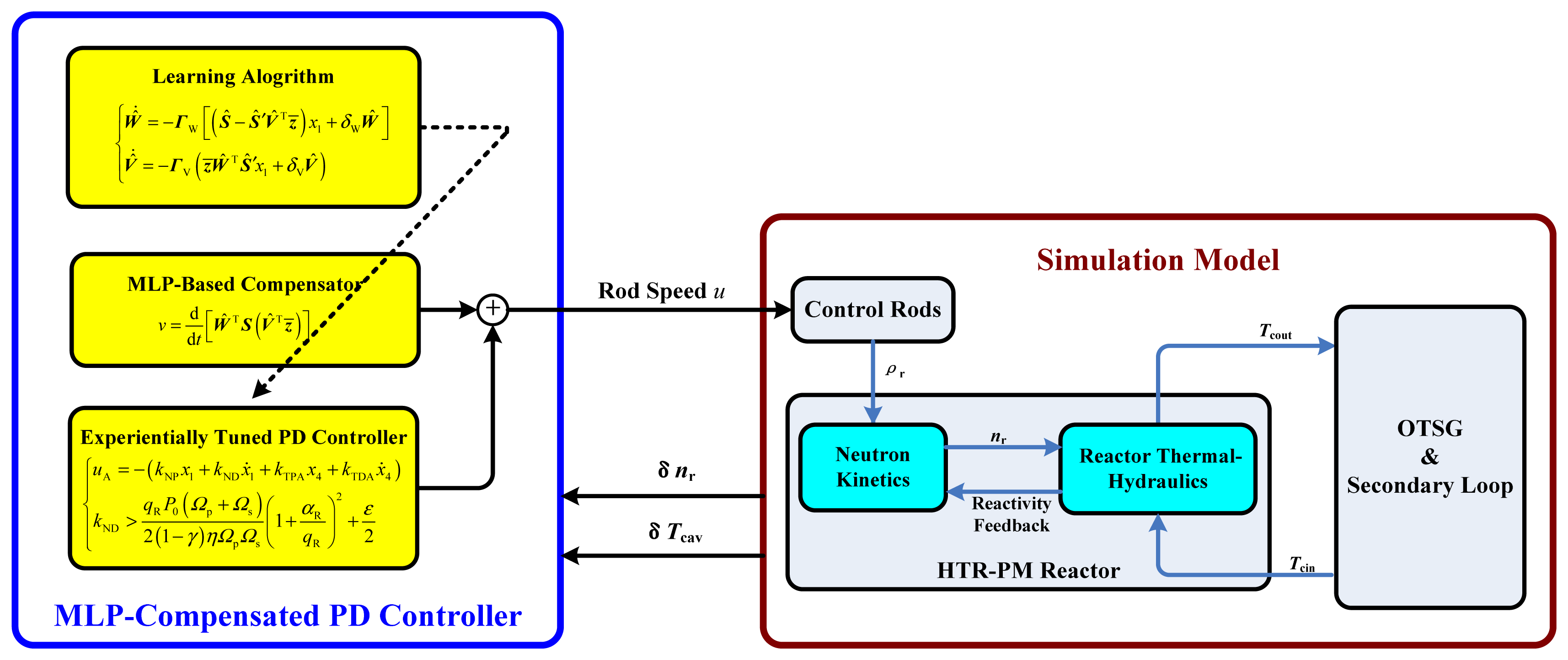
The dynamic model of the MHTGR utilized in this simulation adopts that one composed of both nodal neutron kinetics and nodal reactor thermal-hydraulics given in [39]. The OTSG model is just the moving boundary model presented in [40]. Furthermore, the model of the steam turbine and that of the electrical generator are also included in the simulation code [41]. The schematic view of this NSSS dynamic model for numerical simulation is shown in Figure 3, and the structure of the closed-loop composed of this model and the power-level control strategy proposed in this paper is shown in Figure 4.

Here, in this simulation, we choose those feedback gains of u_A as k_NP = 0.2, k_ND = 0.1, k_TPA = 0.2 and k_TDA = 0.003. Moreover, the parameters of the MLPN utilized for compensation in control strategy in Equation (74) is chosen as l = 3, Γ_W = 1000I₃, Γ_V = 1000I₇, δ_W = δ_V = 0.01, and:

$$\mathit{U}=\text{diag}({\left[\begin{array}{ccccccc}50& 1& 1& 5& 1& 1& 0.01\end{array}\right]}^{\text{T}})$$

(75)

4.2. Simulation Results

In this simulation, two case studies are done to show the feasibility of the above newly-built MLP-compensated PD power-level control law in Equation (74). Moreover, the performance of this new control law is compared with that of the experientially-tuned PD controller u_A given by Equation (31). Here, it is clear that controller in Equation (74) is just experiential control u_A compensated by an MLPN.

(1)

Case A. power-level changes linearly from 100% FP to 50% FP in 10 min.

In this test, the power demand signal decreases down from 100% FP to 50% FP linearly with a speed of 5% FP/min. Due to the drop in power demand, both the error between the actual and demanded nuclear powers and that between the actual and referenced helium temperatures become larger than before.

These error signals drive the power-level controller to insert the control rods. The system enters to a steady state when the reactivity induced by temperature feedback effect is balanced with that given by the control rods. Here, the dynamic responses of the relative nuclear power, average fuel temperature and outlet helium temperature as well as designed control rod speed with and without MLPN compensation are illustrated in Figure 5.

(2)

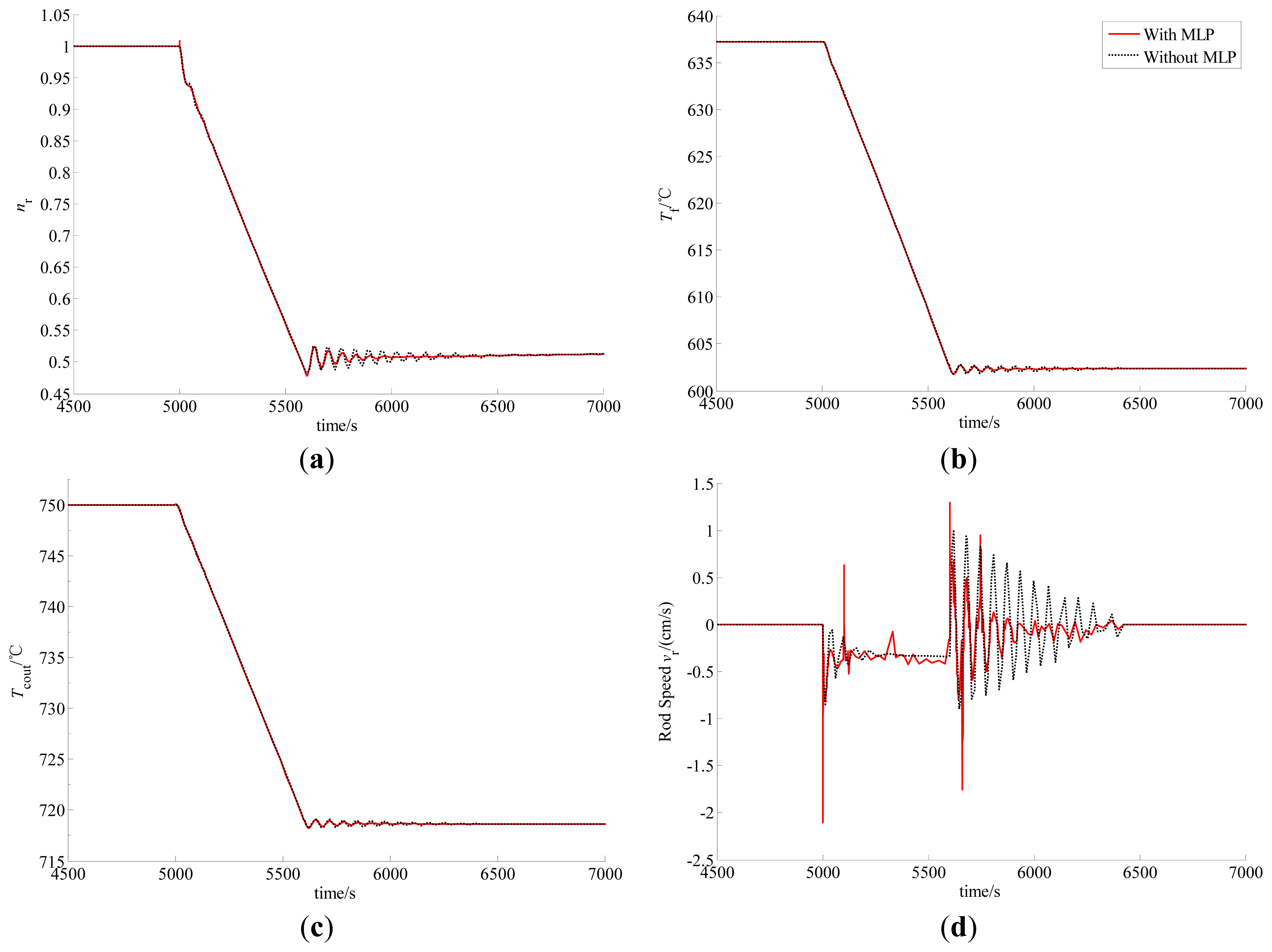
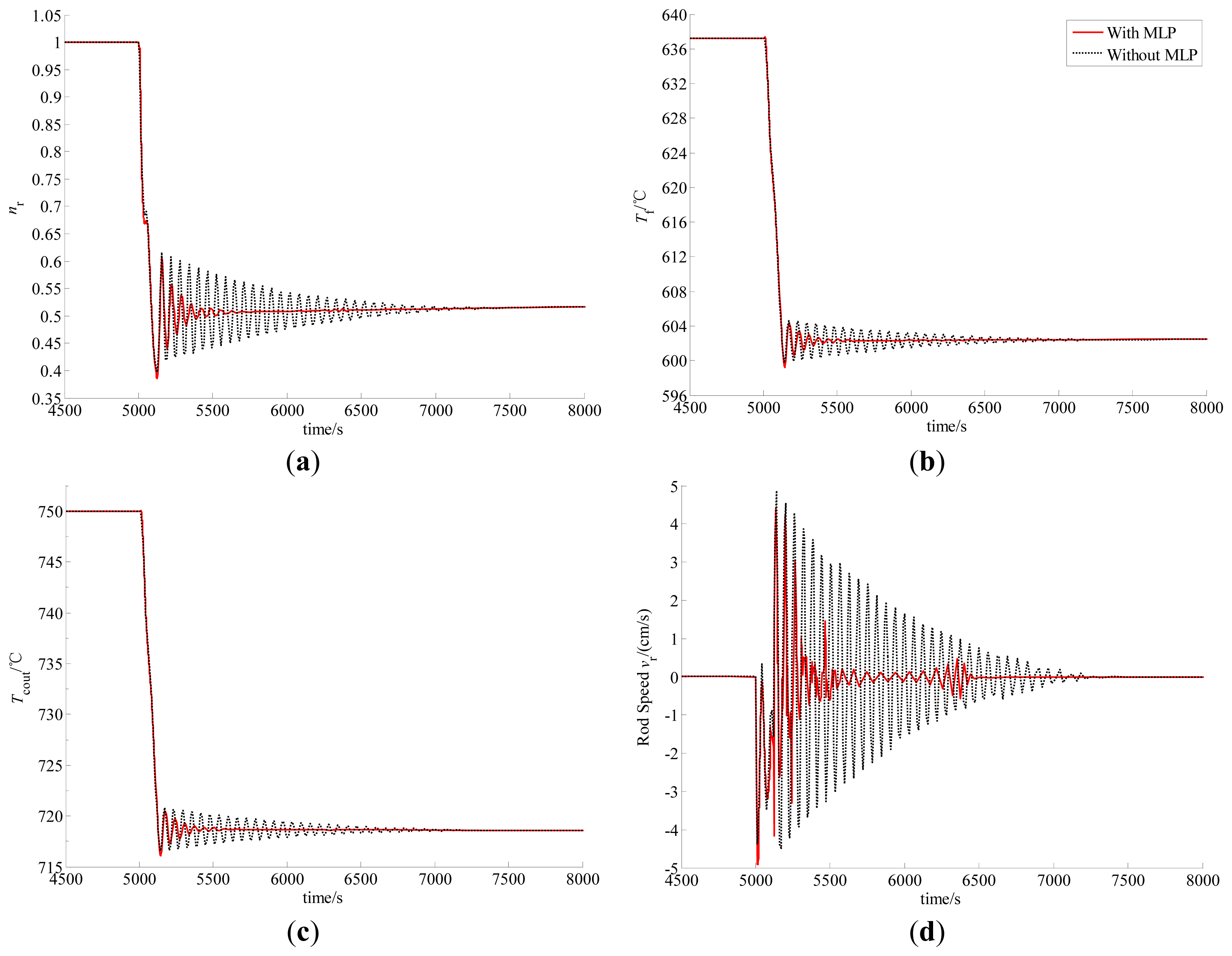
Case B: power-level changes linearly from 100% FP to 50% FP in 2 min.

In this study, the power demand signal decreases linearly from 100% FP to 50% FP in 2 min, and the error signals of the nuclear power and the helium temperature cause the power-level regulator to generate proper rod speed to cope with the decrease of power demand. The computed responses of some crucial reactor process variables and the designed control rod speed with and without the MLPN compensation are all illustrated in Figure 6.

4.3. Discussions

From Figures 5 and 6, we can see that although the closed-loop stability is still guaranteed, there exists oscillation in the dynamic responses of the key process variables. The amplitude of this oscillation is small in the case of slow large-range power maneuvers, and may be acceptable in practical engineering. However, both the amplitude and acting duration are unacceptable in the case of fast large-range power maneuvers. This phenomenon is caused by the parameter uncertainty. Actually, since the real values of some physical and thermal-hydraulic parameters cannot be obtained accurately, we can only tune u_A experientially, which results in parameter uncertainty. Fast variation in the power demand induces large parameter uncertainty, which then leads to strong oscillation of the dynamic responses. Also from Figures 5 and 6, because of the incorporation of the MLPN in the power-level control strategy, the oscillation in the dynamic responses is then quickly and effectively suppressed, especially in the case of fast large-range power maneuvers. This is given by the strong approximation ability of the MLPN. Actually, the oscillations of the process variables quickly excite the learning algorithm of the MLPN weighting matrices to approximate the modal features of this oscillation, and then suppress it by a compensating term in the feedback controller. Thus, the MLPN can be used to cancel the response oscillations by a properly designed learning algorithm.

Finally, from the theoretical analysis and numerical simulation given in Sections 3 and 4, MLP-compensated PD power-level control strategy in Equation (74) not only guarantees the bounded closed-loop stability, but also effectively suppresses the response oscillations caused by parameter mismatch. Furthermore, due to the wide utilization of advanced digital control system platforms, there is no difficulty in realizing MLP-compensated power-level control law in Equation (74). Since there already have been some mature programs of the MLPN, it is easy for engineers to implement MLP-compensated controller in Equation (74) as a software running on the digital platforms. Here, it is worthy to be noted that the power-level control strategy given in this paper is only for the normal power operation of the MHTGR, and NOT for the reactor startup.

5. Conclusions

Due to its inherent safety features and potentially competitive economic power, the MHTGR has already been seen as one of the best candidates in building SMR-based nuclear power plants. It is clear that power-level control of the MHTGR is meaningful in providing safe, stable and efficient operation. Moreover since the MHTGR dynamics have the features of high nonlinearity and parameter uncertainty, this leads to the necessity of developing nonlinear power-level control strategies with strong adaptation capability. Based on the shifted-ectropies of neutron kinetics and reactor thermal-hydraulics, it is firstly proved theoretically that the output-feedback power-level controller with simple PD structure can guarantee the asymptotic closed-loop stability. However, since for tuning this PD control law, we should know the values of some physical or thermal-hydraulic parameters which are difficult to obtain accurately, there must exist parameter uncertainty. Then, an MLPN-based compensator is introduced to deal with the uncertainty. It has been proved theoretically that this newly-built MLP-compensated PD power-level control law can guarantee bounded closed-loop stability. Numerical simulation results in case of large-range power maneuver verify the theoretical results, and show that this MLP compensator can effectively suppress the oscillations caused by system parameter uncertainty. This newly-built power-level regulator can be easily implemented on those advanced digital control system platforms. The main contribution of this paper is proving that simple PD power-level control strategy can provide asymptotic closed-loop stability and designing an MLP-based compensator to suppress the negative influence given by parameter uncertainty.

References

- Ingersoll, D.T. Deliberately small reactors and the second nuclear era. Prog. Nucl. Energy 2009, 51, 589–603. [Google Scholar]
- Vujić, J.; Bergmann, R.M.; Škoda, R.; Miletić, M. Small modular reactors: Simpler, safer, cheaper? Energy 2012, 45, 288–295. [Google Scholar]
- Reutler, H.; Lohnert, G.H. The modular high-temperature reactor. Nucl. Technol. 1983, 62, 22–30. [Google Scholar]
- Reutler, H.; Lohnert, G.H. Advantages of going modular in HTRs. Nucl. Eng. Des. 1984, 78, 129–136. [Google Scholar]
- Lohnert, G.H. Technical design features and essential safety-related properties of the HTR-Module. Nucl. Eng. Des. 1990, 121, 259–275. [Google Scholar]
- Wu, Z.; Lin, D.; Zhong, D. The design features of the HTR-10. Nucl. Eng. Des. 2002, 218, 25–32. [Google Scholar]
- Hu, S.; Liang, X.; Wei, L. Commissioning and Operation Experience and Safety Experiment on HTR-10. Proceedings of the 3rd International Topical Meeting on High Temperature Reactor (HTR) Technology, Johannesburg, South Africa, 1–4 October 2006.
- Zhang, Z.; Sun, Y. Economic potential of modular reactor nuclear power plants based on the Chinese HTR-PM project. Nucl. Eng. Des. 2007, 237, 2265–2274. [Google Scholar]
- Zhang, Z.; Wu, Z.; Wang, D.; Xu, Y.; Sun, Y.; Li, F.; Dong, Y. Current status and technical description of Chinese 2 × 250 MWth HTR-PM demonstration plant. Nucl. Eng. Des. 2009, 239, 265–2274. [Google Scholar]
- Ablay, G. A modeling and control approach to advanced nuclear power plants with gas turbines. Energy Convers. Manag. 2013, 76, 899–909. [Google Scholar]
- Shtessel, Y.B. Sliding mode control of the space nuclear reactor system. IEEE Trans. Aerosp. Electron. Syst. 1998, 34, 579–589. [Google Scholar]
- Dong, Z. Nonlinear state-feedback dissipation power level control for nuclear reactors. IEEE Trans. Nucl. Sci. 2011, 58, 241–257. [Google Scholar]
- Kokotović, P. The joy of feedback. IEEE Control Syst. 1992, 12, 7–17. [Google Scholar]
- Dong, Z.; Feng, J.; Huang, X.; Zhang, L. Dissipation-based high gain filter for monitoring nuclear reactors. IEEE Trans. Nucl. Sci. 2010, 57, 328–339. [Google Scholar]
- Dong, Z.; Huang, X.; Zhang, L. Output-feedback load-following control of nuclear reactors based on a dissipative high gain filter. Nucl. Eng. Des. 2011, 241, 4783–4793. [Google Scholar]
- Maschke, B.M.; Ortega, R.; van der Schaft, A.J. Energy-based Lyapunov functions for forced Hamiltonian systems with dissipation. IEEE Trans. Autom. Control 2000, 45, 1498–1502. [Google Scholar]
- Ortega, R.; van der Schaft, A.J.; Maschke, B.M.; Escobar, G. Interconnection and damping assignment passivity-based control of port-controlled Hamiltonian systems. Automatica 2002, 38, 585–596. [Google Scholar]
- Ortega, R.; van der Schaft, A.J.; Castaños, F.; Astolfi, A. Control by interconnection and standard passivity-based control of port-Hamiltonian systems. IEEE Trans. Autom. Control 2008, 53, 2527–2542. [Google Scholar]
- Dong, Z. Nonlinear dynamic output-feedback power-level control for PWRs: A shifted-ectropy based design approach. Prog. Nucl. Sci. 2013, 68, 223–234. [Google Scholar]
- Dong, Z. PD power-level control design for PWRs: A physically-based approach. IEEE Trans. Nucl. Sci. 2013, 60, 3889–3898. [Google Scholar]
- Na, M.G.; Shin, S.H.; Kim, W.C. A model predictive controller for nuclear reactor power. J. Korean Nucl. Soc. 2003, 35, 399–411. [Google Scholar]
- Tai, Y.; Hou, S.-X.; Li, C.; Zhao, F.-Y. An improved implicit multiple model predictive control used for movable nuclear power plant. Nucl. Eng. Des. 2010, 240, 3582–3585. [Google Scholar]
- Etchepareborda, A.; Lolich, J. Research reactor power controller design using an output feedback nonlinear receding horizon control method. Nucl. Eng. Des. 2007, 237, 268–276. [Google Scholar]
- Eliasi, H.; Menhaj, M.B.; Davilu, H. Robust nonlinear model predictive control for nuclear power plants in load following operations with bounded xenon oscillations. Nucl. Eng. Des. 2011, 241, 533–543. [Google Scholar]
- Eliasi, H.; Menhaj, M.B.; Davilu, H. Robust nonlinear model predictive control for a PWR nuclear power plant. Prog. Nucl. Energy 2012, 54, 177–185. [Google Scholar]
- Dong, Z. Nonlinear adaptive dynamic output feedback power-level control of nuclear heating reactors. Sci. Technol. Nucl. Install. 2013, 2013. [Google Scholar] [CrossRef]
- Ku, C.-C.; Lee, K.Y.; Edwards, R.M. Improved nuclear reactor temperature control using diagonal recurrent neural networks. IEEE Trans. Nucl. Sci. 1992, 39, 2298–2308. [Google Scholar]
- Arab-Alibeik, H.; Setayeshi, S. Adaptive control of a PWR core power using neural networks. Ann. Nucl. Energy 2005, 32, 588–605. [Google Scholar]
- Boroushaki, M.; Ghofrani, M.B.; Lucas, C.; Yazdanpanah, M.J. Identification and control of a nuclear reactor core (VVER) using recurrent neural networks and fuzzy systems. IEEE Trans. Nucl. Sci. 2003, 50, 159–174. [Google Scholar]
- Dong, Z. A neural-network-based nonlinear adaptive state-observer for pressurized water reactors. Energies 2013, 6, 5382–5401. [Google Scholar]
- Li, H.; Huang, X.; Zhang, L. Operation and control simulation of a modular high temperature gas cooled reactor nuclear power plant. IEEE Trans. Nucl. Sci. 2008, 55, 2357–2365. [Google Scholar]
- Dong, Z. Dynamic output feedback power-level control for the MHTGR based on iterative damping assignment. Energies 2012, 5, 1782–1815. [Google Scholar]
- Dong, Z. Physically-based power-level control for modular high temperature gas-cooled reactors. IEEE Trans. Nucl. Sci. 2012, 59, 2531–2548. [Google Scholar]
- Dong, Z. Nonlinear adaptive power-level control modular high temperature gas-cooled reactors. IEEE Trans. Nucl. Sci. 2013, 60, 1332–1345. [Google Scholar]
- Li, H.; Huang, X.; Zhang, L. Simplified mathematical dynamic model of the HTR-10 high temperature gas-cooled reactor with control system design purposes. Ann. Nucl. Energy 2008, 35, 1642–1651. [Google Scholar]
- Ge, S.S.; Huang, C.C.; Lee, T.H.; Zhang, T. Stable Adaptive Neural Network Control; Kluwer Academic Publisher: Norwell, MA, USA, 2002. [Google Scholar]
- Funahashi, K.I. On the approximate realization of continuous mappings by neural networks. Neural Netw. 1989, 2, 183–192. [Google Scholar]
- Zhang, T.; Ge, S.S.; Huang, C.C. Design and performance analysis of a direct adaptive controller for nonlinear systems. Automatica 1999, 35, 1809–1817. [Google Scholar]
- Dong, Z.; Huang, X.; Zhang, L. A nodal dynamic model for control system design and simulation of an MHTGR core. Nucl. Eng. Des. 2010, 240, 1251–1261. [Google Scholar]
- Li, H.; Huang, X.; Zhang, L. A lumped parameter dynamic model of the helical coiled once-through steam generator with movable boundaries. Nucl. Eng. Des. 2008, 238, 1657–1663. [Google Scholar]
- Dong, Z.; Huang, X. Real-Time Simulation Platform for the Design and Verification of the Operation Strategy of the HTR-PM. Proceedings of the 21th International Conference on Nuclear Engineering, Chengdu, China, 29 July–2 August 2013. [CrossRef]
© 2014 by the authors; licensee MDPI, Basel, Switzerland. This article is an open access article distributed under the terms and conditions of the Creative Commons Attribution license ( http://creativecommons.org/licenses/by/3.0/).
Share and Cite
Dong, Z. An Artificial Neural Network Compensated Output Feedback Power-Level Control for Modular High Temperature Gas-Cooled Reactors. Energies 2014, 7, 1149-1170. https://doi.org/10.3390/en7031149
Dong Z. An Artificial Neural Network Compensated Output Feedback Power-Level Control for Modular High Temperature Gas-Cooled Reactors. Energies. 2014; 7(3):1149-1170. https://doi.org/10.3390/en7031149
Chicago/Turabian StyleDong, Zhe. 2014. "An Artificial Neural Network Compensated Output Feedback Power-Level Control for Modular High Temperature Gas-Cooled Reactors" Energies 7, no. 3: 1149-1170. https://doi.org/10.3390/en7031149