Methods to Increase the Robustness of Finite-Volume Flow Models in Thermodynamic Systems

Abstract

This paper addresses the issues linked to simulation failures during integration in finite-volume flow models, especially those involving a two-phase state. This kind of model is particularly useful when modeling 1D heat exchangers or piping, e.g., in thermodynamic cycles involving a phase change. Issues, such as chattering or stiff systems, can lead to low simulation speed, instabilities and simulation failures. In the particular case of two-phase flow models, they are usually linked to a discontinuity in the density derivative between the liquid and two-phase zones. In this work, several methods to tackle numerical problems are developed, described, implemented and compared. In addition, methods available in the literature are also implemented and compared to the proposed approaches. Results suggest that the robustness of the models can be significantly increased with these different methods, at the price of a small increase of the error in the mass and energy balances.

1. Introduction

Dynamic models of thermodynamic systems are very useful for simulating transient conditions, to define, implement and test control strategies or to evaluate and optimize the system response time [1-4]. In particular, two-phase flow models are required for cycles involving evaporation and condensation of the working fluid. For that purpose, finite volume models are among the most widely used.

However, such models are subject to different numerical issues, leading to potentially slow simulation or to simulation failures, and can make the model unusable for some externally imposed operating conditions (e.g., highly transient operation, start-up or shut-down).

One of these issues is chattering, a well-known issue in finite-volumes two-phase flow models. It has been described by various authors, e.g., [3,5], and is due to discontinuities in the model state variables or their derivatives. In the particular case of two-phase flow models, numerical artifacts usually arise from discontinuities in the working fluid thermodynamic properties across the phase boundaries or in the computation of heat transfer.

Flow reversals and/or highly transient system boundary conditions can also result in unsolvable systems of equations, leading, once again, to low simulation speeds or to simulation failures [6].

Solutions to these numerical problems have already been proposed in the literature. One possible solution can be to smooth the discontinuities in the thermodynamic properties, as suggested by [3,5,7]. This was implemented by Bonilla using a Hermite bicubic spline interpolation method, with good results on the chattering problem, but involving a substantial error in the computation of the cell densities [7].

Another solution was originally proposed by Casella et al. [8], consisting in computing a mean density presenting the advantage of being C₁-continuous during phase boundary transitions. This method was tested in [9], showing that it indeed eliminates the chattering problem, with good simulation results and accuracy.

Another proposal consists in numerically removing state variables outside of the part of the state space corresponding to a risk of chattering [10]. This method has proven to reduce the simulation time up to 85% with a limited error, less than 2% in density and 0.6% in specific enthalpy. In [6], an enthalpy limiter method is presented, whose purpose is to avoid an unsolvable system of equations, due to flow reversals or other issues. This imposes a lower boundary on a cell inlet enthalpy and constitutes an effective way to enable the simulation under those critical boundary conditions.

In this paper, a description of the above methods is proposed. Alternative methods are also proposed and described. These methods are then implemented and compared in ThermoCycle, an open-source Modelica library for the modeling of thermal systems [11]. Three different test cases are defined and simulated with the different methods. The comparison criteria are the robustness, the simulation speed, the ability to handle flow reversal, the error on the mass and energy balances and the accuracy of the predicted outputs. Two different discretization schemes are also compared (upwind and central differences) using the same indicators.

Finally recommendations are formulated regarding the use of these different methods with respect to the boundary conditions imposed on the system.

2. Problem Formulation

The models and methods presented here are developed in the Modelica environment. Modelica is well adapted to thermoflow problems, mainly because of its acausal formulation [5]. The proposed models are part of the Modelica ThermoCycle library [1], developed and maintained at the University of Liège. The working fluid thermodynamic properties are obtained using the CoolProp thermodynamic library [12].

This library presents the advantage of being fully open-source and, therefore, allows the implementation of the smoothing methods directly in the thermodynamic properties library.

2.1. Finite Volumes Modeling of Fluid Flows

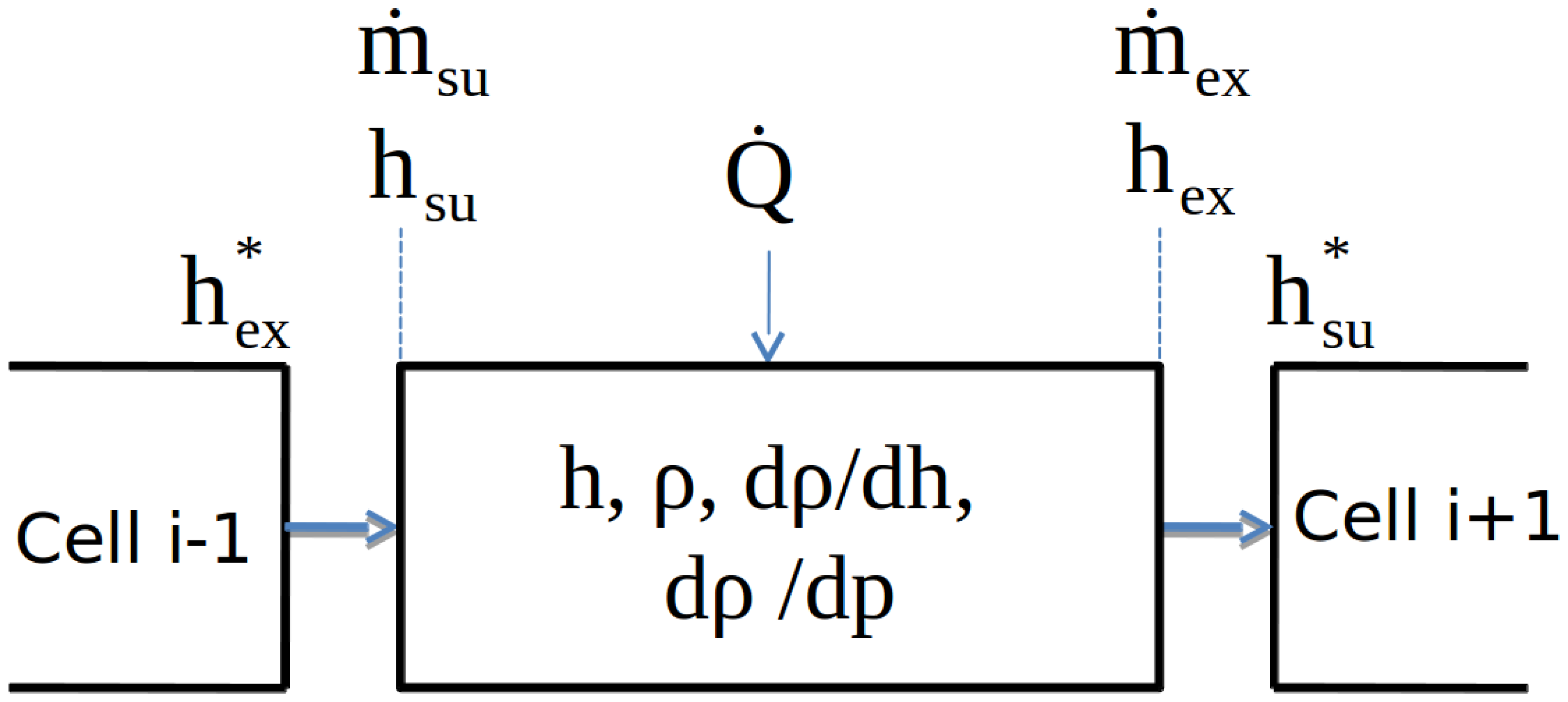
This work focuses on finite volume models of fluid flow (as opposed to, e.g., moving-boundaries models). The flow is discretized into N cells in which the energy and mass conservation equations are applied (see Figure 1). The momentum balance is neglected. The proposed model is a 1D model, i.e., the fluid properties are assumed to vary only in the flow direction.

Two types of variables can be distinguished: cell variables and node variables. Node variables are distinguished by the “su” (supply) and “ex” (exhaust) subscripts and correspond to the inlet and outlet nodes of each cell (Figure 1). The “*” exponent indicates a value relative to the adjacent cell. The mass balance is expressed as a function of the two differentiated state variable (p and h) [13]:

$${ṁ}_{ex}-{ṁ}_{su}=V·\frac{d\rho }{dt}=V·\left(\frac{\partial \rho }{\partial h}·\frac{dh}{dt}+\frac{\partial \rho }{\partial p}·\frac{dp}{dt}\right)$$

(1)

where $\frac{\partial \rho }{\partial h}$ and $\frac{\partial \rho }{\partial p}$ are considered as thermodynamic properties of the working fluid and are computed in CoolProp.

The pressure drop between the inlet and outlet can be computed using the momentum balance [14]:

$$p_{su}-p_{ex}=\frac{V}{A^2}\frac{dṁ}{dt}-\frac{1}{A^2}\left(\frac{{ṁ}_{su}^2}{{\rho }_{su}}-\frac{{ṁ}_{ex}^2}{{\rho }_{cx}}\right)+\mathrm{\Delta }{p}_{\mathit{\text{fric}}}$$

(2)

where A is the channel cross-sectional area and Δp_fric is the pressure drop due to friction. If fast dynamic processes (e.g., sound propagation) are not considered, it is reasonable to neglect the momentum derivative term [14,15]. In the same manner, the momentum fluxes term can also be neglected if the density variation remains limited.

The energy balance is expressed by [13]:

$$V·\rho ·\frac{dh}{dt}={ṁ}_{su}·(h_{su}-h)-{ṁ}_{ex}·(h_{ex}-h)+\dot{Q}+V·\frac{dp}{dt}$$

(3)

where Q̇ is the heat flow to the cell.

The relation between the cell and node values depends on the discretization scheme. In this work, two schemes are implemented: the central difference scheme and the upwind scheme. Since the model accounts for flow reversal, a conditional statement is added depending on the flow rates at the inlet and outlet nodes:

For the central differences scheme, h = (h_su + h_ex)/2, h_su is therefore expressed by (an equivalent equation applies to h_ex):

$$h_{su}=\{\begin{array}{ccccc}{h}_{ex}^{*}& \text{if}& {ṁ}_{su}\ge 0& & \\ 2·h-h_{ex}& \text{if}& {ṁ}_{su}<0& \text{and}& {ṁ}_{ex}<0\\ h& \text{if}& {ṁ}_{su}<0& \text{and}& {ṁ}_{ex}\ge 0\end{array}$$

(4)

where the flow rates are defined as positive when the fluid flows in the nominal direction (from “su” to “ex”) and where $h_{ex}^{*}$ indicates the exhaust node enthalpy of the previous cell.

In the upwind scheme, h = h_su, h_su is therefore expressed by:

$$h_{su}=\{\begin{array}{ccc}h& \text{if}& {ṁ}_{su}<0\\ h_{ex}^{*}& \text{if}& {ṁ}_{su}\ge 0\end{array}$$

(5)

The overall flow model is finally obtained by interconnecting several cells in series. This kind of discretization corresponds to a staggered grid, i.e., the thermodynamics states and the state variables (the enthalpies) are calculated inside the cells and the node values (“su” and “ex”) are deduced using Equations (4) and (5). In a collocated grid, on the contrary, the state variables are the node variables, and the cell variables are deduced.

2.2. Chattering and Flow Reversals

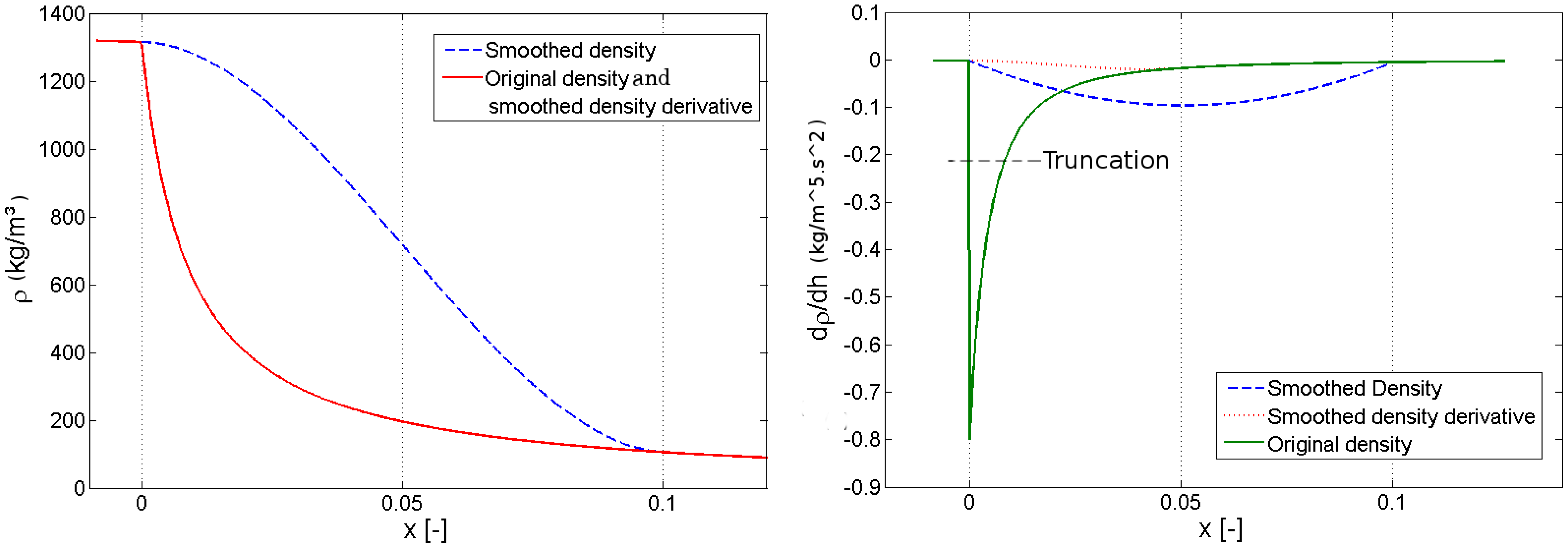
The phenomenon of chattering may occur when discontinuities in the model variables are present [3]. This phenomenon can lead to extremely slow simulation or to simulation failures, because the computed variables exceed acceptable boundaries. In discretized two-phase flow models, the main discontinuity is often the density derivative on the liquid saturation curve (Figure 2). Simulation failure or stiff systems can occur if the cell-generated (and purely numerical) flow rate due to this discontinuity causes a flow reversal in one of the nodes (i.e., the computation of h_su and h_ex switches from one value to the other in Equations (4) and (5).

Flow reversal can result in a singular (i.e., non-solvable) set of equations [6]. This effect can be illustrated with the simple case of a single control volume operating in the following conditions:

• It is assumed that there is one single flow directed towards the control volume. This can, for example, correspond to the situation in which (ṁ_su = 0), and the outlet undergoes a flow reversal, which brings, by convection, an enthalpy imposed by the outer world (ṁ_ex > 0).

• The heat flow to the control volume is assumed to be null or negligible.

When considering a single cell, the addition of working fluid has an effect both on the density in the cell and on its enthalpy. However, a modification of the enthalpy also affects the density in the cell. These two effects can be expressed as a function of an infinitesimal mass addition dm:

$$d\rho =\frac{dm}{V}=\frac{ṁ·dt}{V}>0$$

(6)

where dm is positive, since the considered control volume is assumed to undergo entering flows only due to the flow reversal. With the above hypotheses, the energy balance (Equation (3)) can be simplified into:

$$V·\rho ·dh=dm·(h_{su}-h)+V·dp$$

By combining with Equation (1) to replace dh, the effect of the incoming enthalpy flow on the density can thus be written:

$$\frac{dm}{V}=\frac{\partial \rho }{\partial h}·\frac{1}{\rho }·\frac{dm}{V}·(h_{su}-h)+\frac{\partial \rho }{\partial h}·\frac{1}{\rho }·dp+\frac{\partial \rho }{\partial h}·dp$$

(7)

According to Bridgeman's Table, the two last terms correspond to the equation of an isentropic compression:

$${\left(\frac{\partial \rho }{\partial p}\right)}_s=\frac{\partial \rho }{\partial h}·\frac{1}{\rho }+\frac{\partial \rho }{\partial p}$$

which is a positive term.

Equation (7) can therefore be re-arranged into:

$$\frac{dm}{V}·\left(1-\frac{\partial \rho }{\partial h}·\frac{1}{\rho }·(h_{su}-h)\right)={\left(\frac{\partial \rho }{\partial p}\right)}_s·d\rho$$

(8)

The system of equations related to this control volume is solvable only if the pressure increases (dp > 0) when new fluid is added (dm > 0) [6]. In this case, the right term of Equation (7) is positive, which leads to the following solvability criterion on the enthalpies:

$$h_{su}>h+\frac{\rho }{\frac{\partial \rho }{\partial h}}$$

(9)

where ∂p/∂h is a negative term.

This inequality states that in case of flow reversal, if the enthalpy of the entering fluid is below a certain limit, an unsolvable system of equations appears. A formal and generalized demonstration of this effect can be found in [6].

Therefore, to ensure the robustness of the simulation and to avoid chattering or unsolvable systems, two strategies can be employed:

• Avoid the flow reversals due to the density derivative discontinuity (Equation (1));

• If flow reversal occurs (it is physically possible), make sure that the backflow enthalpy is higher than the limit described in Equation (9).

The first strategy can be expressed by an inequality stating that numerically, cell-generated flow rates must be lower than the flow rate circulating through the cycle, which can be written (for a single cell):

$${ṁ}_{\mathit{\text{ext}}}>>\frac{V}{N}·\frac{d\rho }{dt}=\frac{V}{N}·\left(\frac{\partial \rho }{\partial h}·\frac{dh}{dt}+\frac{\partial \rho }{\partial p}·\frac{dp}{dt}\right)$$

(10)

According to Equation (10), flow reversals and, thus, chattering or simulation failures are likely to occur if:

• The number of cells (N) is low;

• The working fluid flow rate (ṁ_ext) is low;

• The internal volume (V) is high;

• The working conditions are highly transient (i.e., dp/dt and dh/dt are high).

3. Proposed Robustness Methods

This section describes the different methods implemented to avoid the simulation issues described in the previous section. These methods aim at avoiding numerical flow reversal or avoiding unsolvable systems in case a flow reversal occurs.

The different solutions are implemented and tested in the Modelica ThermoCycle library. Some can be implemented at the Modelica level, while others require a modification of the thermodynamic properties of the working fluid. It should also be noted that some of these methods have already been proposed in the literature, while some others are new. The main goal is to compare these different approaches on a common basis, i.e., for the same test cases and using unified comparison criteria.

3.1. Filtering Method

In this strategy, a first-order filter is applied to the fast variations of the density with respect to time:

$$\frac{dy}{dt}=\frac{u-y}{T_{\mathit{\text{filter}}}}$$

(11)

where u and y are the input and output signals, respectively. In this particular case, u is the mass variation calculated with the equation of state (Equation (1)), and y is the filtered mass derivative. This filter therefore acts as the “mass damper” and avoids transmitting abrupt variations of the flow rate due to the density derivative discontinuity. The filtered mass accumulation in each cell is written:

$$\frac{d^{2}m}{d{t}^2}=\frac{V·\left[\frac{\partial \rho }{\partial h}·\frac{dh}{dt}+\frac{\partial \rho }{\partial h}·\frac{dp}{dt}\right]-\frac{dm}{dt}}{T_{\mathit{\text{filter}}}}$$

(12)

where T_filter is the filter time constant, set as the model input. This strategy displaces the mass variations in time, but does not generate mass defects. However, the energy balance is affected, because the cell density is not exactly the one corresponding to the actual node flow rates.

This approach can be implemented at the model level, but doubles the number of time states of the model, since a second-order derivative of the working fluid mass in the cell is defined in Equation (12).

3.2. Truncation Method

This strategy acts on the terms, ∂ρ/∂p and ∂ρ/∂h, of Equation (10). The peak in the density derivative occurring after the transition from liquid to two-phase is truncated, as shown in Figure 2 as a function of the vapor quality (defined as x = (h − h_l)/(h_υ − h_l)). The maximum time derivative of the density is a model parameter, and the maximum partial derivatives are calculated using the following equation:

$$\frac{\partial {\rho }^{\mathit{\text{max}}}}{\partial h}=\frac{d{\rho }^{\mathit{\text{max}}}}{dt}/\frac{d{h}^{\mathit{\text{ref}}}}{dt};\frac{\partial {\rho }^{\mathit{\text{max}}}}{\partial p}=\frac{d{\rho }^{\mathit{\text{max}}}}{dt}/\frac{d{p}^{\mathit{\text{ref}}}}{dt}$$

(13)

The reference values of the time derivatives of p and h are set to a typical value. This allows for the use of a single parameter to compute the two maximum values of the partial derivatives.

This strategy conserves mass balance in each cell, except when a phase transition occurs. In this case, a fictitious creation or destruction of mass appears. Figure 2 shows, however, that the truncated area is relatively limited, which should reduce the mass unbalance. The underlying idea is that a mass defect is acceptable for the simulation if its value is limited and if it significantly increases the robustness of the model. The main advantage of this approach is its easy implementation at the model level, i.e., without modification of the working fluid equation of state.

3.3. Smoothing of the Density Derivative

The idea behind this method is to smooth out the density derivative discontinuity using a spline function, as shown in Figure 2. This can therefore only be performed at the level of the equation of state, i.e., in the thermophysical properties database. Most fluid properties libraries are not open-source, which does not enable the implementation of such a method. However, the CoolProp library [12] is open-source, and its database comprises nearly as many fluids as the Refprop library. It is therefore the one that has been selected for the present work: the smoothing method was implemented in the main code and is now available in the standard distribution of CoolProp.

The main drawback of this method is that the density function is still calculated with the original equation of state; the smoothed density derivative is not consistent with the density function provided by the equation of state. This might cause a mass defect during the simulation.

3.4. Smoothing of the Density Function

In order to avoid the mismatch between the density function and its derivative, one possible solution is to smooth the density for a range of vapor qualities (i.e., making it C₁-continuous) and recalculating its partial derivatives in the smoothed area. In this situation, the density derivatives are continuous, but not smooth, which should still be manageable for the solver.

The density is smoothed using a spline function with respect to the enthalpy between the liquid saturation line and a constant vapor quality line (hereunder referred to by the subscript “x”), as shown in Figure 2. Note that in the equations below, the two independent variables are p and h. For the sake of conciseness, partial derivatives as a function of one of these variables is always assumed to be performed with the other one being constant, although this is not explicitly indicated in the equations.

$${\rho }_{\mathit{\text{smooth}}}=a·{\mathrm{\Delta }}^3+b·{\mathrm{\Delta }}^2+c·\mathrm{\Delta }+d\text{for}0<\mathrm{\Delta }<{\mathrm{\Delta }}_x$$

(14)

where Δ is the difference between the current enthalpy and the saturated liquid enthalpy at the given pressure:

$$\mathrm{\Delta }=h-h_l;{\mathrm{\Delta }}_x=x·(h_{\upsilon }-h_l)$$

The spline coefficients, a, b, c and d, are given by:

$$\begin{array}{c}a=\frac{1}{{\mathrm{\Delta }}_x^3}·\left[2·{\rho }_l-2·{\rho }_x+{\mathrm{\Delta }}_x·({\frac{\partial \rho }{\partial h}|}_l+{\frac{\partial \rho }{\partial h}|}_x)\right]\\ b=\frac{3}{{\mathrm{\Delta }}_x^2}·({\rho }_x-{\rho }_l)-\frac{1}{{\mathrm{\Delta }}_x}·(2·{\frac{\partial \rho }{\partial h}|}_l+{\frac{\partial \rho }{\partial h}|}_x)\\ c={\frac{\partial \rho }{\partial h}|}_l\\ d={\rho }_l\end{array}$$

Since the partial derivative of Δ with respect to h is equal to one; the partial derivative of the smoothed density function with respect to h is straightforward:

$$\frac{\partial {\rho }_{\mathit{\text{smooth}}}}{\partial h}=3a·{\mathrm{\Delta }}^2+2b·\mathrm{\Delta }+c$$

(15)

The partial derivative with respect to p requires more terms, since the spline coefficients depend on p and must also be differentiated.

$$\frac{\partial {\rho }_{\mathit{\text{smooth}}}}{\partial p}=(3a·{\mathrm{\Delta }}^2+2b·\mathrm{\Delta }+c)·\frac{\partial \mathrm{\Delta }}{\partial p}+\frac{da}{dp}·{\mathrm{\Delta }}^3+\frac{db}{dp}·{\mathrm{\Delta }}^2+\frac{dc}{dp}·\mathrm{\Delta }+\frac{dd}{dp}$$

(16)

with:

$$\begin{array}{c}\frac{da}{dp}=\frac{6}{{\mathrm{\Delta }}_x^4}·\frac{d{\mathrm{\Delta }}_x}{dp}·({\rho }_x-{\rho }_l)+\frac{2}{{\mathrm{\Delta }}_x^3}·(\frac{d{\rho }_l}{dp}-\frac{d{\rho }_x}{dp})+\frac{1}{{\mathrm{\Delta }}_x^2}·({\frac{{\partial }^2\rho }{\partial h\partial p}|}_l+{\frac{{\partial }^2\rho }{\partial h\partial p}|}_x)-\frac{2}{{\mathrm{\Delta }}_x^3}·(\frac{d{\rho }_l}{dh}+\frac{d{\rho }_x}{dh})·\frac{d{\mathrm{\Delta }}_x}{dp}\\ \frac{db}{dp}=\frac{6}{{\mathrm{\Delta }}_x^3}·\frac{d{\mathrm{\Delta }}_x}{dp}·({\rho }_x-{\rho }_l)+\frac{3}{{\mathrm{\Delta }}_x^2}·(\frac{d{\rho }_x}{dp}-\frac{d{\rho }_l}{dp})+\frac{1}{{\mathrm{\Delta }}_x^2}·\frac{d{\mathrm{\Delta }}_x}{dp}·({2·\frac{\partial \rho }{\partial h}|}_l+{\frac{\partial \rho }{\partial h}|}_x)-\frac{1}{{\mathrm{\Delta }}_x}·({\frac{{\partial }^2\rho }{\partial h\partial p}|}_x+{2·\frac{{\partial }^2\rho }{\partial h\partial p}|}_l)\\ \frac{dc}{dp}={\frac{{\partial }^2\rho }{\partial h\partial p}|}_l\\ \frac{dd}{dp}=\frac{d{\rho }_l}{dp}\end{array}$$

and:

$$\begin{array}{c}\frac{d{\mathrm{\Delta }}_x}{dp}=x·(\frac{d{h}_{\upsilon }}{dp}-\frac{d{h}_l}{dp})\\ \frac{\partial \mathrm{\Delta }}{\partial p}=-\frac{d{h}_l}{dp}\\ \frac{d{\rho }_x}{dp}={\rho }_x^2·(\frac{x}{{\rho }_{\upsilon }^2}·\frac{d{\rho }_{\upsilon }}{dp}+\frac{1-x}{{\rho }_l^2}·\frac{d{\rho }_l}{dp})\end{array}$$

All the other partial or total derivatives can be obtained from the Bridgeman Tables. They are implemented in the standard distribution of CoolProp [12] and are summarized in [16].

Equations (14)–(16) are therefore used instead of the original equation of state in the area of the thermodynamic diagram characterized by a vapor quality varying between zero and x. x is a parameter of the model and is set by default to 0.1.

3.5. Mean Densities Method

The mean densities method was originally proposed by Casella [8] and successfully tested by Bonilla et al. [9]. It is also the method implemented in the ThermoPower Modelica library [2].

The goal is to avoid the numerical artifact, due to the density derivative discontinuity crossing one of the finite volumes boundaries. To that end, a mean density and its partial derivatives are computed in each cell as a function of the node densities. The main advantage is that the discontinuity in the partial derivatives disappears. Nine different equations of the mean density are proposed, corresponding to nine possible situations: h_su and h_ex can both either be liquid, two-phase or vapor. The total number of combinations is therefore equal to nine. As an example, in the case where h_su is liquid and h_ex is two-phase, the mean density is computed by:

$$\begin{array}{c}\overline{\rho }=\frac{1}{h_{ex}-h_{su}}\left[\frac{{\rho }_{su}+{\rho }_l}{2}(h_l-h_{su})+\frac{h_{\upsilon }-h_l}{{\upsilon }_{\upsilon }-{\upsilon }_l}ln\left(\frac{{\rho }_l}{{\rho }_{ex}}\right)\right]\\ \frac{\partial \overline{\rho }}{\partial h}=\frac{{\rho }_{ex}-{\rho }_{su}}{h_{ex}-h_{su}}\\ \frac{\partial \overline{\rho }}{\partial h}=\frac{1}{h_{ex}-h_{su}}\left[\frac{1}{2}\left(\frac{\partial {\rho }_{su}}{\partial p}+\frac{\partial {\rho }_l}{\partial p}\right)(h_l-h_{su})+A·ln\left(\frac{{\rho }_l}{{\rho }_{ex}}\right)+B({\rho }_l-{\rho }_{ex})\right]\end{array}$$

where A and B are functions of the fluid thermodynamic properties on the liquid and vapor saturation lines. The equations for the eight other cases, as well as the analytical expression of A and B are available in [8,9].

It should be noted that this approach requires the computation of the node densities. As a consequence, a staggered grid should not be used, since it would require twice as many thermodynamic state computations (in the cells and in the nodes), which would considerably increase the simulation time. Therefore, to implement this method, the staggered grid described in the previous section was changed to a collocated grid (i.e., the thermodynamic states are only computed at the nodes).

3.6. The Enthalpy Limiter Method

Contrary to the previous methods, the enthalpy limiter method does not aim at avoiding flow reversals. Instead, it ensures that the system of equations remains solvable even in case of flow reversal. As indicated in Equation (9), the enthalpy of the fluid entering a cell should have a minimum value, ensuring that the system of equations can be solved. The enthalpy limiter method is the practical implementation of this constraint in the cell model. It was originally proposed by Schultze et al. and implemented in the TIL Modelica library.

The idea is to make profit of the “Stream” connector type available in Modelica to propagate the minimum enthalpy limitation: in this manner, a cell can communicate with its two neighboring cells and propagate the minimum enthalpy of an incoming flow according to Equation (9). The incoming flow is limited to this minimum value:

$$h_{\mathit{\text{limit}},i}=h_i+0.9·\frac{{\rho }_i}{\frac{\partial {\rho }_i}{\partial h}}$$

(17)

In the two adjacent cells, the enthalpy of the outlet flow is given by (example for i-1):

$$h_{ex,i-1}=max(h_{\mathit{\text{limit}},i},h_{i-1})$$

(18)

A security factor of 0.9 is taken to ensure a minimum distance between the outlet enthalpy and the theoretical limit.

Details regarding the practical implementation of this method in Modelica are available in [6].

3.7. Smooth Reversal Enthalpy

In Equation (5), a discontinuity appears in the computed node enthalpy in the case of flow reversal. This can be solved using a smooth transition between both parts of the equation. Equation (5) is therefore transformed into:

$$h_{su}=\{\begin{array}{ccc}h& \text{if}& {ṁ}_{su}\le -\frac{{ṁ}_{\mathit{\text{nom}}}}{10}\\ h+\frac{h_{ex}^{*}-h}{2}·\left[1+sin(\frac{5·\pi }{{ṁ}_{\mathit{\text{nom}}}}ṁ)\right]& \text{if}& -\frac{{ṁ}_{\mathit{\text{nom}}}}{10}<{ṁ}_{su}<\frac{{ṁ}_{\mathit{\text{nom}}}}{10}\\ h_{ex}^{*}& \text{if}& {ṁ}_{su}\ge \frac{{ṁ}_{\mathit{\text{nom}}}}{10}\end{array}$$

(19)

The smooth transition is a C₁-continuous sinusoidal transition function varying from zero to one between −ṁ_nom/10 and −ṁ_nom/10 and available in ThermoCycle. ṁ_nom is a user-defined model parameter.

4. Comparison and Benchmarking of the Different Methods

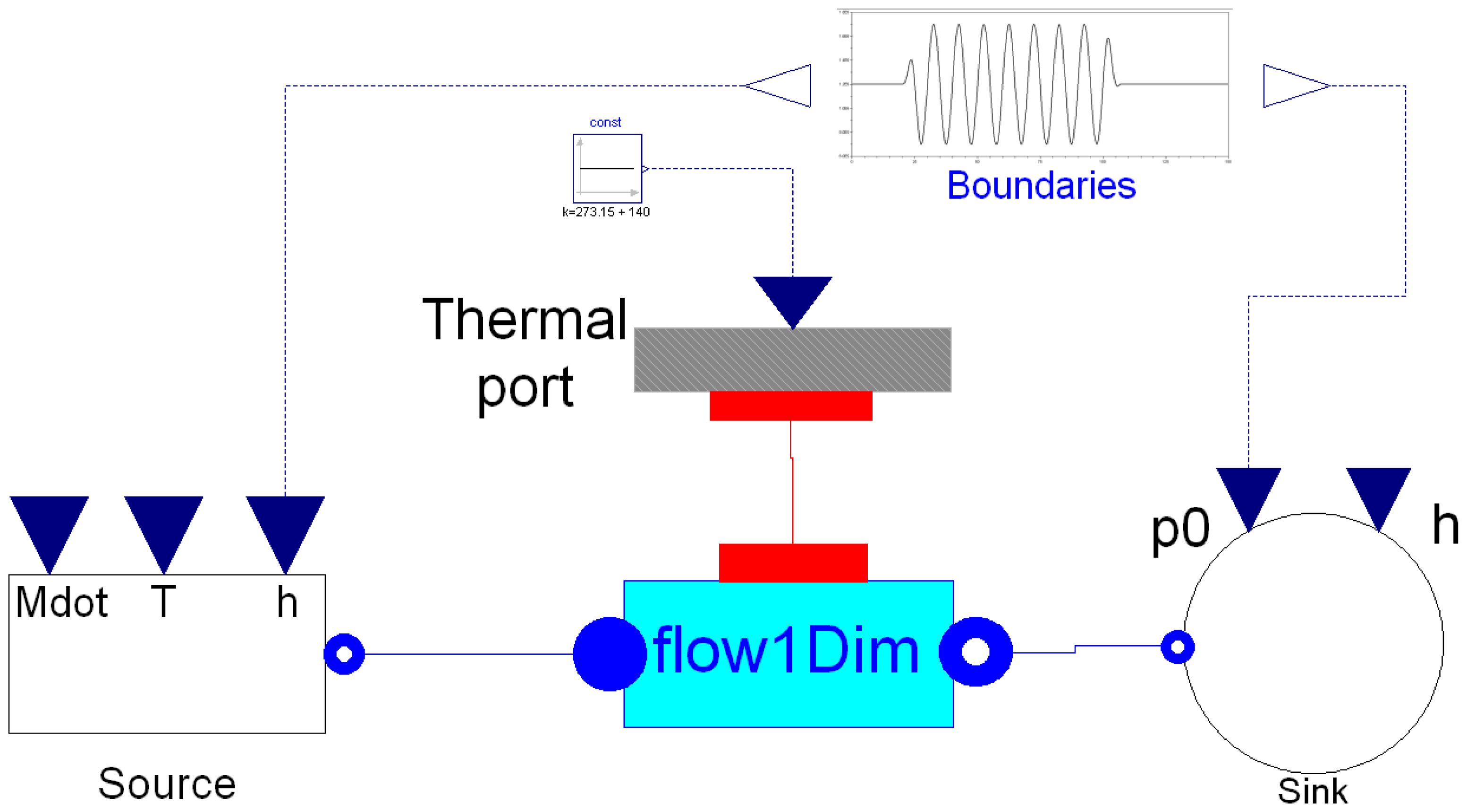
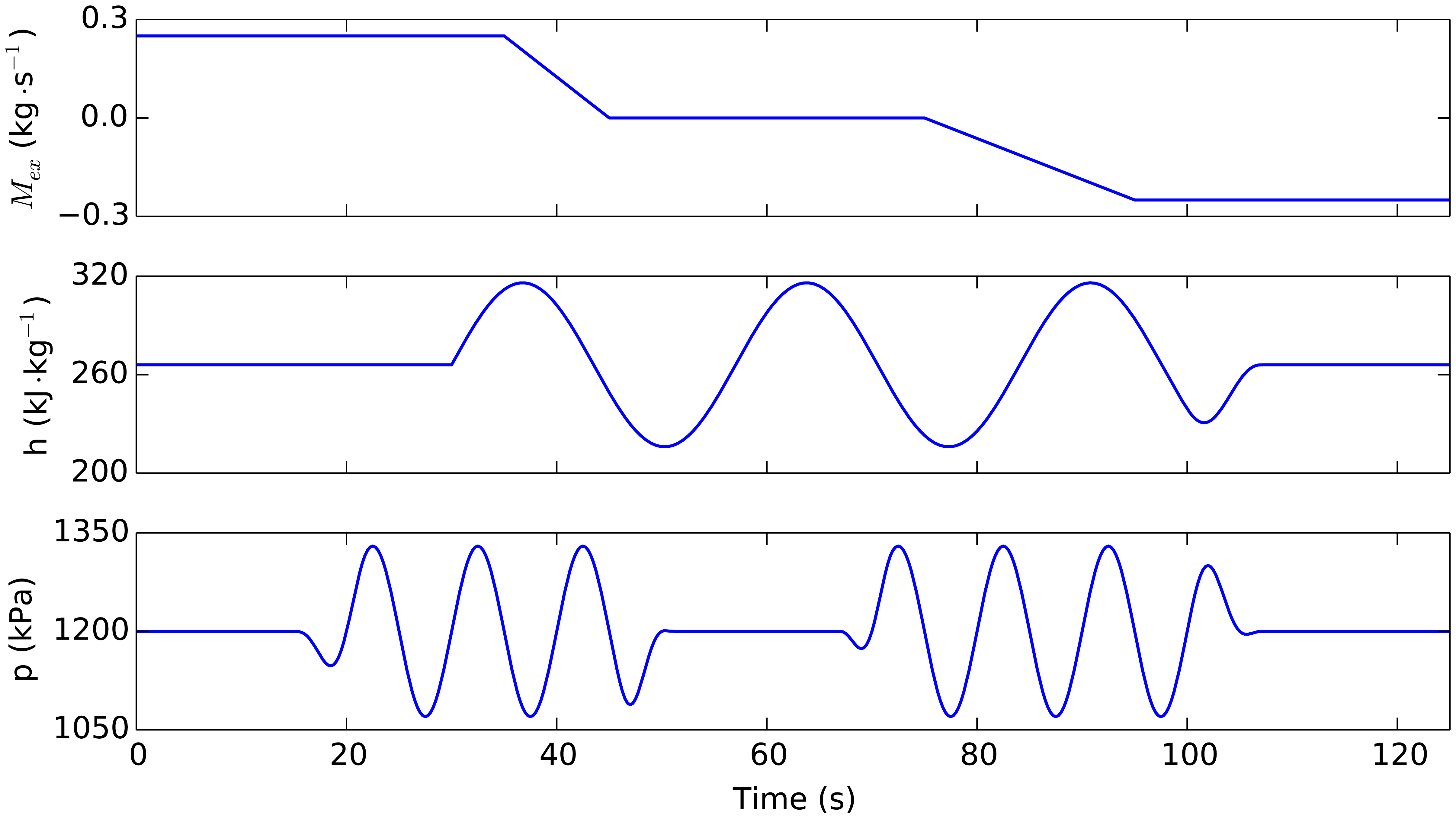
To test and compare the different methods presented above, a reference system is defined, comprising a working fluid flow being evaporated by a constant-temperature heat source, a working fluid source and a working fluid sink. In this system, the two-phase fluid flow is submitted to highly transient conditions by varying its pressure and inlet enthalpy (Figure 3). The pressure drop is assumed to be null (Equation (2)) since its influence on the numerical issues described above is negligible. The detailed system characteristics are provided in

Table 1. Characteristics of the reference system.

Parameter	Variable Name and Value
Working fluid	R245fa
Pipe internal volume	V = 0.004 m3
Number of cells	N = 20
Source flow rate	ṁext = 0.25 kg/s
Heat source temperature	Ths = 140 °C
Heat transfer coefficient	U = 500 W/m2K
Heat transfer area	A = 1.2 m2

.

The simulation is initialized in the steady state and lasts 125 s. After 100 s, the pressure and enthalpy inputs are imposed at their constant initial value to bring the system back to the steady state at the end of the simulation.

4.1. Benchmarking Indicators

The comparison criteria between the proposed methods are presented hereunder.

4.1.1. Mass and Energy Balance

As stated above, the methods involving a modification (truncation, filtering, smoothing) of the density derivatives might generate non-physical artifacts, e.g., create mass and energy unbalances. This is checked by computing the mass and energy balances over the whole simulation period using the following equations:

$${\mathit{\varepsilon }}_{\mathit{\text{ener}}}=\frac{\underset{t}{\mathit{\int }}[\dot{Q}-({ṁ}_{ex}{h}_{ex}-{ṁ}_{su}{h}_{su})]dt-\text{∑}_1^N(U_{i,\mathit{\text{final}}}-U_{i,\mathit{\text{init}}})}{\underset{t}{\mathit{\int }}\dot{Q}dt}$$

(20)

$${\mathit{\varepsilon }}_{\mathit{\text{mass}}}=\frac{\underset{t}{\mathit{\int }}({ṁ}_{ex}-{ṁ}_{su})dt-\text{∑}_1^N{V}_i({\rho }_{i,\mathit{\text{final}}}-{\rho }_{i,\mathit{\text{init}}})}{\underset{t}{\mathit{\int }}{ṁ}_{su}dt}$$

(21)

4.1.2. Accuracy

The accuracy is defined as the agreement of the model-predicted output values (the outlet enthalpy and flow rate) with a reference system. The selected reference system is the same as the one presented in Figure 3, but with a high number of cells (100 in this case). The reference system is run with the upwind discretization scheme, and the selected mathematical indicator is the coefficient of determination (R²) between ṁ_ex,ref and ṁ_ex,ref and between h_ex,ref and h_ex,pred (i.e., the two model outputs).

4.1.3. Computational Efficiency

The computational efficiency of a method is evaluated by the CPU time required for the integration.

4.1.4. Flow Reversal Capability

Most finite volume models present the capability to handle reverse flow. However, few of them are able to handle flow reversal (i.e., switching from a positive flow rate to a negative one). As mentioned before, this is an important feature, since flow reversals are likely to occur either because of numerical artifacts (Equation (10)) or because the flow reversal is imposed by the process. This capability is also related to the ability of the system to handle zero flow. This is especially important when simulating start-up or shut-down conditions.

4.1.5. Robustness

In the present work, robustness is defined as the ability of the model to simulate the system without failure. To assess this ability, the amplitude of the variations of the boundary conditions are multiplied by a factor, α, which is progressively increased until reaching a simulation failure. Therefore, models capable of running without failure with high α values are considered to be the most robust.

5. Simulation Results and Discussion

To characterize the different finite volumes approaches, the simple model described above is submitted to three different boundary conditions sets, representative of different practical situations in which such models are likely to be used.

5.1. Speed Test

This first test aims at characterizing the simulation speed of the different methods. To that end, the system presented in Figure 3 is submitted to enthalpy and pressure variations, but these variations are limited to avoid any back-flow or state event generation. As a consequence, none of the above-presented methods should undergo any simulation failure in this test. The boundary conditions for pressure and enthalpy are defined as follow:

$$p=12+\alpha ·1.3·sin(0.1·2\pi ·t)[\text{bar}]$$

(22)

$$h_{su}=2.66·{10}^5+\alpha ·5·{10}^4·sin(0.9·2\pi ·t)[\text{J}/\text{kg}]$$

(23)

$$h_{\mathit{\text{backflow}}}=6·{10}^5[\text{J}/\text{kg}]$$

(24)

where the parameter, α, is a multiplicator that increases the amplitude of the transients to which the system is submitted. For the present test, it is set to one. h_{back flow} is the enthalpy of the fluid coming out of the sink component in the case of flow reversal. Enthalpy values are referenced to 200 kJ/kg for saturated liquid at 273.15 K.

Table 2. Simulation results of the speed test.

Method	Discretization	tCPU (s)	εener (%)	εmass (%)	${\mathit{R}}_{\mathit{\text{flow}}}^{\mathbf{2}}\mathbf{(}\mathbf{\%}\mathbf{)}$	${\mathit{R}}_{\mathit{h}}^{\mathbf{2}}\mathbf{(}\mathbf{\%}\mathbf{)}$
Standard—100 cells	Upwind	124.0	0.11	0.07	100.0	100.0
Standard	Upwind	9.5	0.81	0.32	91.0	96.6
Standard	Central differences	10.2	0.44	0.20	98.5	99.3
Filtering	Upwind	27.6	1.23	0.26	30.0	53.3
Filtering	Central differences	40.6	2.27	0.18	46.6	66.6
Truncation	Upwind	4.7	2.24	0.80	0.0	21.2
Truncation	Central differences	4.9	2.76	1.03	47.2	53.6
Smooth density derivative	Upwind	6.2	0.16	0.07	40.2	47.7
Smooth density derivative	Central differences	5.7	0.13	0.08	73.6	69.4
Smooth density	Upwind	6.0	0.47	0.15	88.4	94.9
Smooth density	Central differences	6.1	0.14	0.01	83.3	98.5
Mean densities	Upwind	5.2	0.20	0.25	86.4	94.2
Enthalpy limiter	Upwind	9.1	0.36	0.15	91.1	96.9
Smooth reversal enthalpy	Upwind	8.8	0.98	0.38	91.8	96.6

shows that, using the standard model, the error on the mass and energy balances varies between 0.2% and 0.3% and between 0.4% and 0.8%, respectively, depending on the discretization scheme. These figures, although small, are not negligible. It should be noted that the selected numerical relative tolerance for the integration algorithm (DASSL) is set to 10⁻⁴. Setting the tolerance to 10⁻⁶ significantly reduces the error (between 0.02% and 0.07% for the energy and between 0.009% and 0.011% for the mass). In this case, the simulation time is multiplied by a factor close to 10 (46.6 s for the upwind scheme and 49.5 s for the central differences scheme). Since 10⁻⁴ is the default value used in most simulations, the reference error values will be the ones related to this tolerance. It should also be noted that simulation speed can vary between different simulations of the same model. The maximum stated difference was about 0.5 s. The provided simulation times should therefore be considered as indicative only.

The following conclusions can be drawn from Table 2:

• The central difference scheme is more accurate (higher R²) than the upwind scheme, both for the standard model and coupled to the proposed numerical methods.

• The simulation speeds for both discretization schemes are very similar.

• There is no straightforward correlation between mass and energy unbalances (ε) and accuracy (R²). High ε is therefore a necessary, but not sufficient, condition for a valid simulation.

• A comparison between the different methods in terms of computational efficiency leads to the following ranking (from the fastest to the slowest): truncation, mean densities, smoothing of the thermodynamic properties, smooth reversal enthalpy, standard, filtering. Most robustness methods therefore increase the model computational efficiency, except for the filtering method. This is due to the higher number of state variables for this latter method, because of the second-order time derivative (Equation (12)).

• The mass and energy unbalances are acceptable for most numerical methods. Most of the proposed robustness methods present a lower error on the balance than the standard model, with the exception of the filtering and truncation methods, in which the unbalance becomes significant. These two methods should therefore be avoided.

• The lowest unbalance is obtained for the smoothed density method with the central differences scheme.

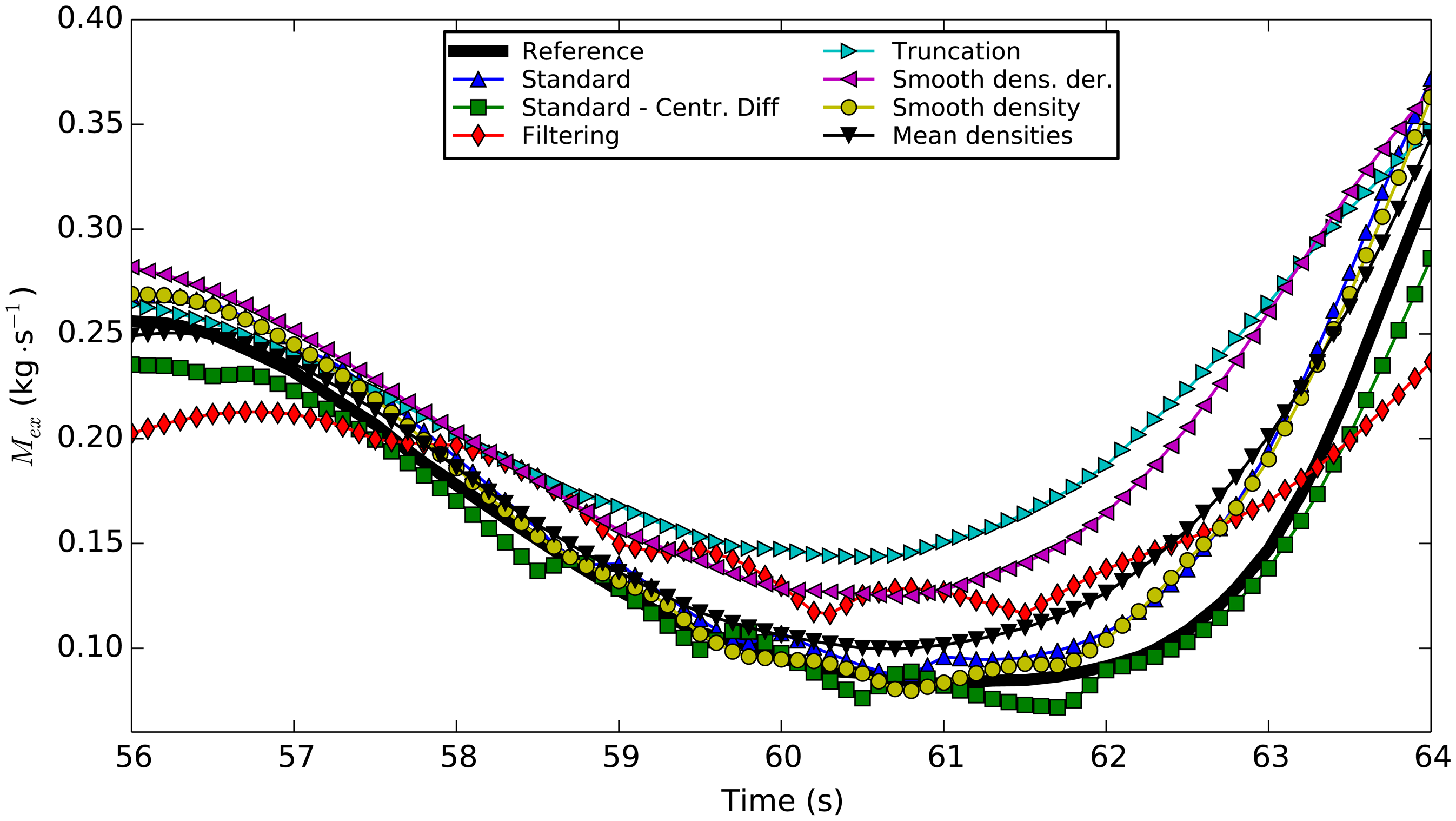
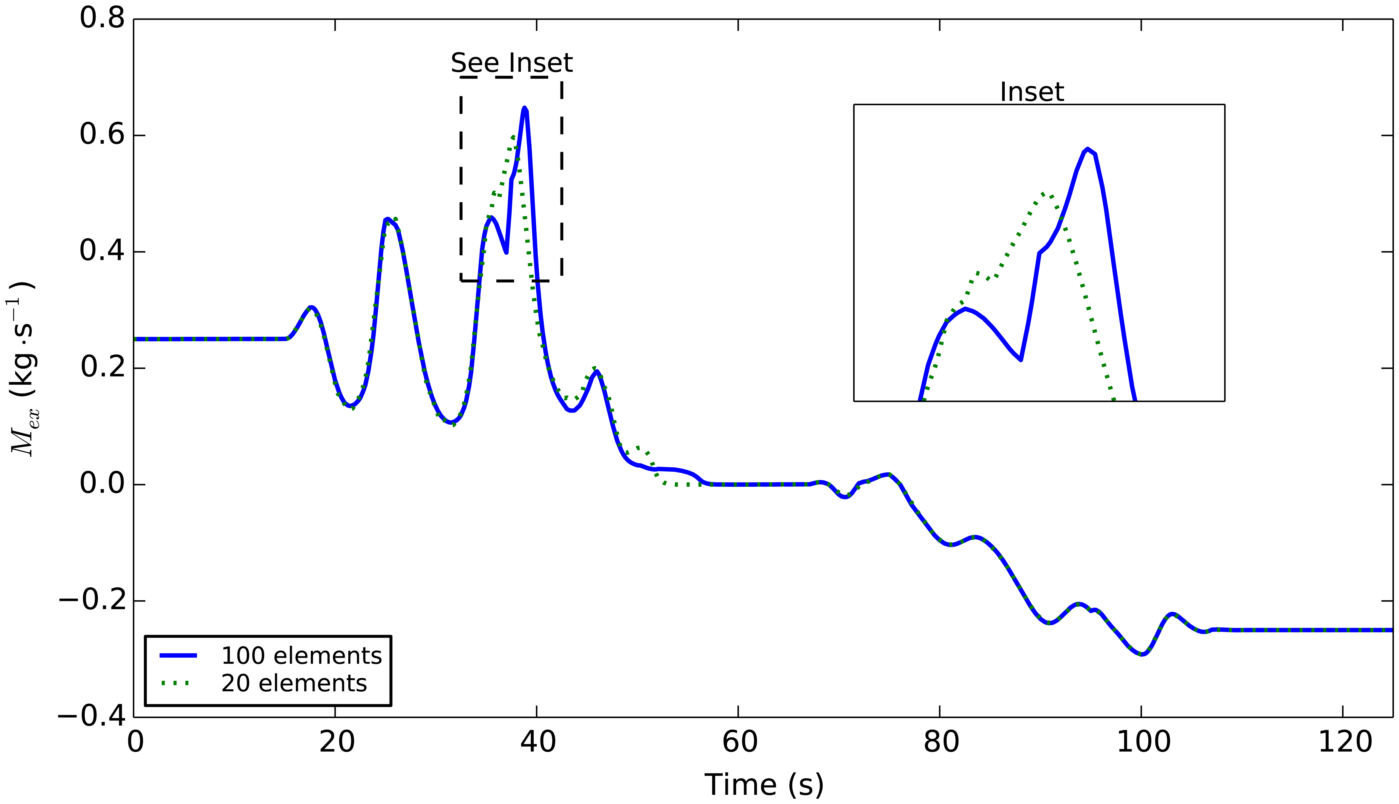
• The accuracy of the different methods is variable, as illustrated in Figure 4. The smooth reversal enthalpy and the enthalpy limiter method present the same accuracy as the standard method, since the models are equivalent in the absence of flow reversal. The most accurate model is, as expected, the standard model, followed by the smooth density method, the mean densities, the smooth density derivative, the filtering method and the truncation method. It should be noted that the two latter methods present very low R² values for both outputs and should therefore be avoided.

• As shown in Figure 4 for a highly transient part of the simulation, the differences between the predicted exhaust flow rates are significant. The profiles that match best the reference profile are the standard model, the smooth density method and the mean densities method. The standard model (both upwind and central differences) undergoes abrupt changes in the predicted flow rate, each of which correspond to a cell crossing the liquid saturation line (and, thus, numerically generating a cell flow rate). With the smooth density method, the variations are lower, while they totally disappear with the mean densities method.

5.2. Flow Reversal Test

This test evaluates the ability to handle zero flow and flow reversal. To that end, the imposed working fluid flow rate is decreased from 0.25 to zero; zero flow is maintained for 30 s and reversed from zero to −0.25. The boundary conditions are described in Figure 5. During zero flow conditions, h_su and p are set to constants to evaluate the ability to simulate standstill conditions. For this simulation, the only accuracy indicator taken into account is the $R_{\mathit{\text{flow}}}^2$ (the prediction of the outlet flow), since after reversal, the enthalpy at the outlet is imposed by the sink and not predicted by the model anymore.

Simulations results are presented in

Table 3. Simulation results of the reversal test.

Method	Discretization	tCPU (s)	εener (%)	εmass (%)	$R_{\mathit{\text{flow}}}^2(\%)$
Standard—100 cells	Upwind	114.0	0.10	0.05	100.0
Standard	Upwind	9.4	0.28	0.15	98.9
Filtering	Upwind	12.5	0.90	0.10	97.9
Filtering	Central differences	42.7	1.56	0.05	98.3
Truncation	Upwind	6.5	7.76	3.45	97.3
Smooth density derivative	Upwind	6.5	7.15	3.21	97.7
Smooth density	Upwind	8.4	0.06	0.04	98.8
Enthalpy limiter	Upwind	6.7	2.47	0.18	98.9
Smooth reversal enthalpy	Upwind	8.5	0.26	0.15	98.9

and in Figure 6. It should be noted that the mean densities method is not suitable for flow reversal and could therefore not be included in the present analysis. The central difference scheme methods also present numerical issues at zero flow (except with the filtering method, but with a prohibitive simulation time). Is is also interesting to note that the comments formulated for the speed test are still valid for the reversal test: lower accuracy of the filtering and truncation method, lower simulation time for most implemented methods compared to the standard model, low energy and mass conservation errors with the smooth density method, etc. In addition, the following comments can be expressed:

• The enthalpy limiter method creates an artifact on the energy balance and, therefore, results in a slightly higher error.

• The smooth density derivative method involves substantial errors and a lower accuracy.

5.3. Robustness Test

In this test, the same system as in the speed test is simulated. However, the amplitude of the pressure and enthalpy variations is multiplied by a factor, α, whose value is increased by steps of 0.25, until a simulation failure occurs. The value of α is then taken as the robustness criterion to compare the different methods.

Table 4. Simulation results of the robustness test.

Method	Discretization	α (−)	εener (%)	εmass (%)
Standard	Upwind	3	0.4	0.3
Standard	Central differences	1.5	2.3	0.7
Filtering	Upwind	9	45.6	1.1
Filtering	Central differences	4	25.5	0.6
Truncation	Upwind	8.5	17.9	5.8
Smooth density derivative	Upwind	7.25	6.7	3.3
Smooth density derivative	Central differences	1.5	0.5	0.1
Smooth density	Upwind	5.5	5.5	3.1
Smooth density	Central differences	2	0.6	0.4
Mean densities	Upwind	4	36.8	4.6
Enthalpy limiter	Upwind	6	24.6	1.2
Smooth reversal Enthalpy	Upwind	2.75	4.0	1.6

presents the simulation results. It shows that all the proposed methods can significantly increase the robustness of the simulation, except the smooth reversal enthalpy method. Even though the errors cannot be directly compared, since the boundary conditions are not equal for all simulation, the following conclusions can be drawn:

• The central difference scheme is less robust than the upwind scheme, which is most likely due to its inability to handle flow reversals, as shown in the previous section.

• The classification of the proposed methods in terms of increased robustness leads to the following chart (here, for the upwind scheme): filtering, truncation, smooth density derivative, enthalpy limiter, smooth density, mean densities standard, smooth reversal enthalpy.

• However, the balance errors linked to these methods are significantly high, especially for the energy balance. This is due to the fact the the model is run at its limits, where a large number of numerical artifacts occur, such as the activation of the enthalpy limiter, or very high numerically generated flow rates. The associated error on the energy balance can be as high as 45.6% in the case of the filtering method, which is explained by the very variability of the heat source (a = 9) in this case.

6. Conclusions

This paper presents different strategies to improve the robustness of finite volume models for two-phase flows. Different strategies are defined and described, originating from the scientific literature (mean densities, enthalpy limiter, smooth reversal enthalpy) or newly developed for the purpose of this work (smoothing methods, truncation, filtering). In particular, some of the developed strategies could only be implemented by modifying the implementation of the working fluid equation of state. This was made possible by the use of CoolProp, which is, to our knowledge, the first comprehensive open-source thermophysical properties library. The proposed methods can therefore be implemented for a large variety of working fluids. The main conclusions related to each of these methods are summarized in

Table 5. Summary of the different methods.

Method	Speed	Robustness	Error	Accuracy	Recommended use
Filtering	−	++	−−	−−	Not recommended
Truncation	++	++	−−	−−	Not recommended
Smooth density derivative	+	++	+	±	If the smooth density method is not sufficient
Smooth density	+	+	++	++	To avoid the discontinuity in the liquid saturation line
Mean densities	++	±	+	++	Systems without flow reversal
Enthalpy limiter	+	+	±	+	Systems submitted to flow reversals
Smooth reversal Enthalpy	+	−−	−	+	Not recommended

.

In all the tests, using a first-order filter or a truncation for the density derivative leads to a much higher error on the mass and energy balances (up to 45%) and to a very low accuracy. These two methods are therefore not recommended. Smoothing the density derivative instead of the density function leads to a higher robustness, but a low accuracy. This is due to the fact that in the second case, the density function and it derivatives are consistent, which reduces artifacts in the mass balance. The mean densities method presents very interesting characteristics in terms of speed, error and accuracy. However, its main drawback is the incapacity to simulate flow reversal. It is, however, very computationally efficient and presents a low mass and energy balance error in usual operation (i.e., avoiding highly transient operation). When flow reversals are unavoidable, the enthalpy limiter method is very useful to ensure that the system remains solvable. However, by limiting the enthalpy, it generates an artifact that causes significant errors on the energy balance.

The simulations have also shown that the central difference scheme is more accurate than the upwind scheme in usual operation. However, its robustness is limited, because of its inability to handle flow reversals.

As shown in the simulations, it is interesting to see that even if numerical artifacts are generated, the error remains of the same order of magnitude as the error linked to the standard finite volume model with a 10⁻⁴ tolerance. This is an important statement showing that the proposed models can ensure failure-free simulation, even in highly transient conditions. A direct validation of the proposed methods with experimental data is out of the scope of this paper, but the limited error in comparison with the standard model (which has been validated by various authors) tends to demonstrate that their accuracy is acceptable. It should also be noted that the transient conditions likely to generate chattering or stiff systems are usually concentrated in specific times of the simulation (e.g., start-up and shut-down), in which robustness is more important than accuracy.

References

- Fritzson, P. Principles of Object-Oriented Modeling and Simulation with Modelica 2.1; John Wiley & Sons: Piscataway, NJ, USA, 2010. [Google Scholar]
- Casella, F.; Leva, A. Modelica Open Library for Power Plant Simulation: Design and Experimental Validation. Proceeding of the 2003 Modelica Conference, Linköping, Sweden, 3–4 November 2003.
- Jensen, J.M. Dynamic Modeling of Thermo-Fluid Systems: With Focus on Evaporators for Refrigeration. Ph.D. Thesis, Energy Engineering, Department of Mechanical Engineering, Technical University of Denmark, Kongens Lyngby, Denmark, 2003. [Google Scholar]
- Quoilin, S.; Aumann, R.; Grill, A.; Schuster, A.; Lemort, V.; Spliethoff, H. Dynamic modeling and optimal control strategy of waste heat recovery Organic Rankine Cycles. Appl. Energy 2011, 88, 2183–2190. [Google Scholar]
- Tummescheit, H. Design and Implementation of Object-Oriented Model Libraries Using Modelica. Ph.D. Thesis, Lund Institute of Technology, Lund, Sweden, 2002. [Google Scholar]
- Schulze, C.; Gräber, M.; Tegethoff, W. A limiter for preventing singularity in simplified finite volume methods. Math. Model. 2012, 7, 1095–1100. [Google Scholar]
- Bonilla, J.; Yebra, L.; Dormido, S. Chattering in dynamic mathematical two-phase flow models. Appl. Math. Model. 2012, 36, 2067–2081. [Google Scholar]
- Casella, F. Object-Oriented Modelling of Two-Phase Fluid Flows by the Finite Volume Method. Proceedings of the 5th Mathmod, Vienna, Austria, 8–10 February 2006; pp. 6–8.
- Bonilla, J.; Yebra, L.J.; Dormido, S. Mean densities in dynamic mathematical two-phase flow models. Comput. Model. Eng. Sci. (CMES) 2010, 67, 13–37. [Google Scholar]
- Bonilla, J.; Yebra, L.; Dormido, S. A heuristic method to minimise the chattering problem in dynamic mathematical two-phase flow models. Math. Comput. Model. 2011, 54, 1549–1560. [Google Scholar]
- Quoilin, S.; Desideri, A.; Bell, I.; Wronski, J.; Lemort, V. Robust and Computationally Efficient Dynamic Simulation of Orc Systems: The Thermocycle Modelica Library. Proceedings of the 2nd International Seminar on ORC Power Systems, Rotterdam, The Netherlands, 7–8 October 2013.
- Bell, I.H.; Wronski, J.; Quoilin, S.; Lemort, V. Pure- and Pseudo-Pure Fluid Thermophysical Property Evaluation and the Open-Source Thermophysical Property Library CoolProp. Ind. Eng. Chem. Res. 2014, 53, 2498–2508. [Google Scholar]
- Quoilin, S. Sustainable Energy Conversion Through the Use of Organic Rankine Cycles for Waste Heat Recovery and Solar Applications. Ph.D. Thesis, University of Liege, LiÃĺge, Belgium, 2011. [Google Scholar]
- Richter, C. Proposal of New Object-Oriented Equation-Based Model Libraries for Thermodynamic Systems. Ph.D. Thesis, University of Braunschweig, Braunschweig, Germany, 2008. [Google Scholar]
- O'Kelly, P. Computer Simulation of Thermal Plant Operations; Springer: New York, NY, USA, 2012. [Google Scholar]
- Thorade, M.; Saadat, A. Partial derivatives of thermodynamic state properties for dynamic simulation. Environ. Earth Sci. 2013, 70, 3497–3503. [Google Scholar]