Evaluation of Visitor Counting Technologies and Their Energy Saving Potential through Demand-Controlled Ventilation

Abstract

Direction-sensitive visitor counting sensors can be used in demand-controlled ventilation (DCV). The counting performance of two light beam sensors and three camera sensors, all direction sensitive, was simultaneously evaluated at an indoor location. Direction insensitive sensors (two mat sensors and one light beam sensor) were additionally tested as a reference. Bidirectional counting data of free people flow was collected for 36 days in one-hour resolution, including five hours of manual counting. Compared to the manual results, one of the light beam sensors had the most equally balanced directional overall counting errors (4.6% and 5.2%). The collected data of this sensor was used to model the air transportation energy consumption of visitor counting sensor-based DCV and constant air volume ventilation (CAV). The results suggest that potential savings in air transportation energy consumption could be gained with the modeled DCV as its total daily airflow during the test period was 54% of the total daily airflow of the modeled CAV on average. A virtually real-time control of ventilation could be realized with minute-level counting resolution. Site-specific calibration of the visitor counting sensors is advisable and they could be complemented with presence detectors to avoid unnecessary ventilation during unoccupied periods of the room. A combination of CO₂ and visitor counting sensors could be exploited in DCV to always guarantee sufficient ventilation with a short response time.

1. Introduction

People flow rate means the number of people passing a specific location during a selected time interval. It is measured using a visitor counting sensor triggered by physical signals caused by the passing person such as visual appearance, heat emission, reflections of the body surface, or pressure against the floor [1]. Building maintenance applications of visitor counting include monitoring customer circulation patterns in commercial facilities [2] and determining the number of people occupying a certain zone. The zone population information can be further used in automatic control of environmental settings, such as demand-controlled ventilation (DCV) that responds to changes in the generation rate of indoor pollutant by adjusting ventilation rate [3,4]. Ventilation recommendations are usually given in outdoor airflow rates per person, and during unoccupied periods the system can be turned to minimum flow settings or totally shut off [5]. Thus a DCV can provide an acceptable indoor air quality and energy savings [5–7]. The most notable benefits are achieved in overventilated facilities and in rooms with high and varying populations, and where the occupants are the main source of indoor air contaminants [8,9]. While a DCV that operates by monitoring the room's carbon dioxide (CO₂) level or temperature is always more or less retrospective, the use of visitor counting sensors enables a real-time response to changing occupancies. For statistical counting of visitors the direction insensitive sensors are also applicable, but in zone population detection bidirectional counting is practically always needed.

Previous research on sensor-based DCV has focused on CO₂ sensor-controlled solutions. The previous studies point out that significant energy savings can be reached using a sensor-based DCV instead of constant air volume (CAV) ventilation [4,8]. Mysen et al. [4] evaluated the energy consumption of a CO₂ sensor-based and infrared (IR) occupancy sensor-based DCV at class rooms during a regular school day. Compared to a CAV, the CO₂ sensor-based DCV reduced the energy use of ventilation to 38% and the IR occupancy sensor-based DCV to 51% [4]. Nassif [10] proposed a robust CO₂ sensor-based DCV strategy. Its performance was compared to a calculation by ASHRAE Standard 62.1 procedure for variable air volume system supplying conditioned air to typical two-story office buildings in seven USA locations with different climate. With occupancies less than 50% of the room design occupancy, the saving in cooling energy could be up to 23% [10]. Norbäck et al. [11] compared the computer class rooms with CAV and with a CO₂ sensor-based DCV. It was found out that the DCV system may slightly reduce headache and tiredness of the room occupants and improve the perceived air quality. It was, however, noticed that there was also high levels of pet allergens in the class rooms that were possibly home-originated and attracted by the electrostatic effects of the computer monitors [11]. In the evaluation of a CO₂ sensor-based DCV by Fan et al. [12] in an open-type office in Japan, approximately a 30% energy saving compared to CAV was noticed.

Benezeth et al. [13] proposed an algorithm for a video camera-based system for indoor occupant presence detection and activity analysis. The system was evaluated at an office room and a corridor setting, yielding people detection accuracies of about 93% and 83%, respectively [13]. Naghiyev et al. [14] compared occupancy detection methods for domestic environments. They were based on passive infrared (PIR) sensors, CO₂ sensors and a device-free localization (DfL) that exploited irregularities in existing Wi-Fi network caused by room occupants. Use of advanced algorithms or a combination of several occupancy detection methods was suggested to compensate the slow response time of CO₂ sensors. The detection capabilities of the PIR sensor-based system could be improved by increasing the sensor density. It was mentioned as a benefit of the DfL that it needs no additional hardware. More research, however, is still needed for proper exploitation of the method [14]. Yang et al. [15] presented an energy saving ventilation control system exploiting temperature sensors. The computer based system modified the velocity of the ventilation fans according to the environmental temperature; for example for temperatures of 10 °C and 38 °C the used fan speeds were 1.7 m/s and 5.5 m/s, respectively [15]. Zamora-Martínez et al. [16] described an indoor temperature forecasting system based on artificial neural networks. The system utilized various sensors inputs, including CO₂, humidity and temperature. As the preliminary tests showed that maintaining the current temperature used only 30%–38.9% of the energy needed to lower the temperature, an accurate forecasting of the indoor temperature could be exploited in energy efficient control of the indoor conditions [16].

In a visitor counting sensor-based DCV knowledge of the sensor's performance is of great importance, as the more reliable the data it provides, the better the results in the application utilizing it. Many commercial sensors claiming to be high in accuracy are also high in price [17], but any specification about the conditions under which the promised accuracy can be reached is seldom available. Literature-based surveys comparing properties of different brands of sensors and sensor technologies include a study by Bu et al. [18]. The survey included IR beam and PIR counters, a piezoelectric pad, a laser scanner and computer vision systems [18]. Previous sensor comparisons including experimental testing of the devices have mostly been performed outdoors. A sensor survey undertaken by SRF Consulting Group, Inc. [19] included four commercial sensors suitable for both pedestrian and bicycle detection: microwave, video camera, and IR sensors, and a combined passive IR and ultrasonic sensor. Turner et al. [20] performed an evaluation test of three IR sensors with varying target speed, distance, group spacing and sensor mounting height. Yang et al. [17] tested the accuracy of a passive IR counter and an IR camera counter at a trail, a sidewalk, a crosswalk and a pedestrian bridge. Bauer et al. [21] evaluated an IR beam sensor and a switching mat sensor in counting passengers and inferring checkpoint service times at the Vienna airport in Austria. Kuutti et al. tested the accuracy of four different video and IR overhead camera sensors at an indoor location using predetermined patterns of two and three people [22].

Although manual counting results—gathered either on site or from video recordings—are commonly used as a ground-truth reference when evaluating the accuracy of a visitor counting sensor, the method undeniably has its limitations. Counting complex pedestrian crowds correctly can be difficult and the manual counting process is tedious, thus being prone to error due to constraints in the counter's ability to maintain attention. Manual data is also typically collected only for a short period of time, which makes generalizing the results over the entire sensor operation time somewhat unreliable [23]. The accuracy of different manual counting methods suitable for sensor calibration—bookkeeping with paper sheets and hand held clickers and counting from video recordings—has been evaluated among others by Anberger and Hinterberger [24] and Diógenes et al. [25].

In the first part of this study the counting performance of five direction sensitive sensors was evaluated simultaneously at the same indoor counting site. Additionally three direction insensitive sensors were included in the test as a comparison for the non-direction results of the direction sensitive sensors. The test included side-mounted light-beam sensors, overhead camera sensors and floor-installed sensor mats. Generally speaking, image processing-based camera sensors should be both accurate and high in counting capacity, as being overhead-installed they are able to detect multiple people entering the counting site simultaneously. However, they are more expensive (€500–2500) compared to lower capacity side-mounted light beam sensors (€50–200) or floor-assembled mat sensors (about €400). Thus multiple sensor technologies were tested to find out if the camera sensors provided a benefit for the visitor counting. The individual technologies and brands were selected based on their availability. For statistical analysis, the counting data was collected for 36 days with a one-hour resolution. During this period, five one-hour bidirectional manual counting sessions were made for sensor counting error analysis.

In the second part of the study the gathered test data was used to model changes in energy consumption of air transportation if a visitor counting sensor-based DCV was used to control a test room's ventilation instead of CAV. Based on the sensor test results the counting data of the most promising bidirectional visitor counting sensor was used. The set point for the modeled CAV was selected according to a time-weighted average zone population of the room.

2. Materials and Methods

2.1. Sensors Included

The visitor counting sensors included in the test setup are presented in

Table 1. Sensors included to the test setup. The direction insensitive sensors are shaded in gray color.

Category	Description	Model	Manufacturer	Origin (city, country)
Light beam	Triangulation proximity switch (IR)	TPS 210	Cedes	Landquart, Switzerland
Light beam	Background suppression sensor (IR)	DL-S202 a	Takex/Teknovisio	Kyoto, Japan/Parainen, Finland
Camera	Network camera	M3203 b	Axis	Lund, Sweden
Camera	Stereoscopic camera	PCN-1001	Eurotech	Amaro, Italy
Camera	Thermal camera	IRC3020	Irisys	Northampton, UK
Mat	Piezoelectric mat	L-series c	Emfit	Jyväskylä, Finland
Mat	Switching mat	SMS 4 d	Schmersal	Wuppertal, Germany
Light beam	IR photocell with reflector	DES-700	Yu-Heng Electric	Kaohsiung, Taiwan

^aCustom made by Teknovisio Ltd. (Parainen, Finland) of two sensor modules and a direction sorting circuit;^bWith embedded Cognimatics True View people counting software;^cMat size 1200 × 580 mm;^dMat size 1000 × 500 mm.

. All sensors, except the network camera, provided counting pulse outlets utilized for data acquisition in the test setup. All tested camera sensors came with their own setup software.

The direction sensitive light beam sensors (a triangulation proximity switch and a background suppression sensor) featured two separately adjustable infrared beams in the same housing with built-in signal processing. These sensors recognized the movement direction of a passing person from the interruption order of the beams and sent a pulse to the corresponding output channel.

The object detection and direction discrimination of the camera sensors (a network camera, a stereoscopic camera and a thermal camera) was based on processing the captured video or infrared images. Two virtual counting lines perpendicular to the movement direction were defined in the sensor's embedded counting software. As a passer-by completely crossed the counting lines in a certain order the movement direction was recognized and a counting pulse was sent to the corresponding channel.

Although sensitivity of movement direction is in practice essential in building maintenance applications, also direction-insensitive sensors (a piezoelectric mat, a switching mat and an IR photocell with reflector) were included in the tests. The non-directional readings of the direction sensitive sensors were obtained by totaling the corresponding directional readings. Thus the counting results of the direction-insensitive sensors could be used to find out the possible effect of direction discrimination on the counting accuracy. Unlike the light beam and mat sensors the camera sensors were capable of detecting people passing them side-by-side.

2.2. Test Site and Sensor Displacement

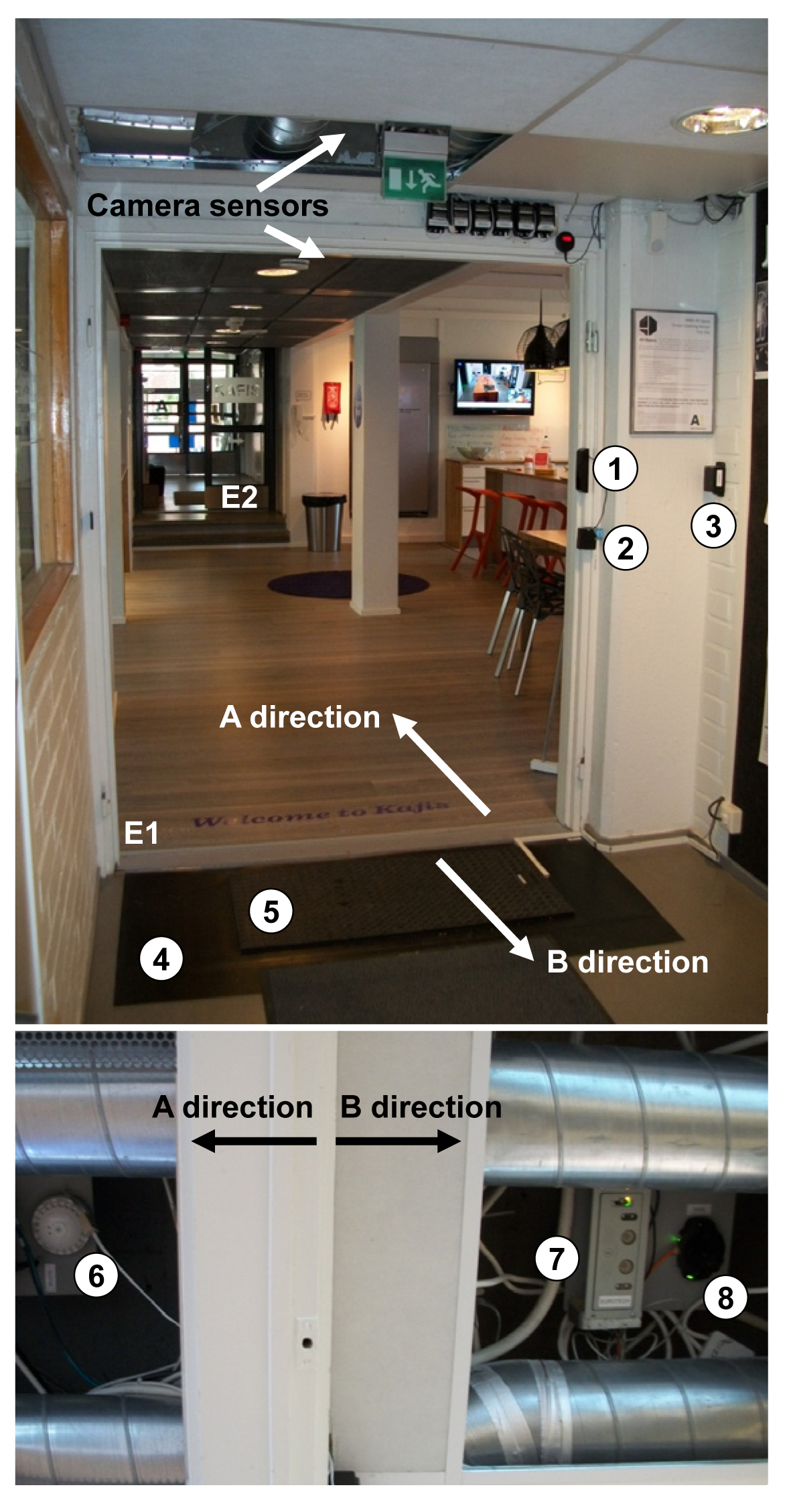
The location for the test setup was a doorway between the Café room and a meeting room corridor in the Aalto Design Factory building in Espoo, Finland. The site's physical dimensions were considered suitable for the sensor installations: the width and height of the doorway were 156 cm and 198 cm, respectively. There also were no doors that could possibly affect the sensors. Based on empirical experience, the passage was also known to be one of the busiest in the building.

The sensors were installed at the test site following the manufacturer and vendor instructions. The placement of the sensors and the counting directions A and B are presented in Figure 1. The piezoelectric mat sensor was placed on the corridor side of the door threshold between two shielding rubber mats. The switching mat sensor was placed on top of the piezoelectric mat. The installation heights of the light beam sensors were as follows (measured from the bottom of the casing): the triangulation proximity switch 123 cm, the background suppression sensor 125 cm and the IR photocell with reflector 104 cm. Distances between the camera sensors and the floor were 244 cm for the network camera, 243 cm for the stereoscopic camera and 260 cm for the thermal camera. Because the ventilation ducts would otherwise have blocked the cameras' fields of view the camera sensors were mounted on two 30 cm high mounting brackets, the network camera and the stereoscopic camera on the first and the thermal camera on the second one. The brackets were then installed in a single file of about 1.5 m in length along the corridor direction, the one holding the network camera and stereoscopic camera on the corridor side, and the thermal camera on the Café side of the doorway (below in Figure 1).

2.3. Data Acquisition

For data collection and power supply, all test sensors except the network camera were connected to Teknovisio Ltd.'s (Parainen, Finland) Visit Log 4000 GSM data loggers. One logger included four pulse-channel interfaces and as the direction insensitive and sensitive sensors reserved one and two channels respectively, altogether four loggers were needed. The counting data was collected with a one-hour resolution and the readings were sent once a day to the Visit Service server. For the direction sensitive sensors both counting directions were registered separately and added up to get the non-directional samples. For quick checking of the proper function of the sensors, digital indicators were connected between the sensors and loggers and mounted above the doorway on the corridor side.

The network camera was connected through an Ethernet connection to a local computer stationed in a private office. The counting results in one-hour intervals were afterwards downloaded from the sensor using an internet browser. The Visit Service system used Finnish standard time which was also used to synchronize the network camera with rest of the system. The network camera had no external indicators at the test site.

Verification of the proper operation of the test setup was done along with the installation and configuration of the devices. Patterns of one and—when applicable—two persons walking side-by-side and one behind the other were used. The completed setup was used to collect round-the-clock counting data for 36 days, yielding altogether 863 sensor-specific one-hour samples (one sample was lost due to changing to daylight saving time) for both directions, when applicable. During the data collection no manipulated patterns of passers-by were used but people were freely allowed to walk through the test site.

For sensor performance evaluation a manual on-site control counting was additionally carried out in five one-hour periods. Two volunteers were seated in suitable locations on both sides of the test site doorway, each monitoring and counting only one of the two walking directions. By doing this, any problems stemming from one person trying to monitor two directions simultaneously were avoided. The manual monitors used simple four-digit hand-held counters to register the passers-by. The manual results were double-checked from the video recording that was captured using the network camera sensor.

2.4. Evaluation of the Sensors' Counting Accuracy

2.4.1. Sensor Counting Error Rates

The counting accuracies of the test sensors were evaluated against the real time manual control results by calculating a counting error rate (ε) for the sensor specific readings (in percentage):

$$\varepsilon =\frac{S-M}{M}\times 100\%$$

(1)

where S is the hourly sensor reading and M the corresponding manual ground truth reference of the control counting period. After this an overall error rate (E) for every sensor was calculated as (in percentage):

$$E=\frac{1}{5}\sum _{i=1}^5\left|{\varepsilon }_i\right|$$

(2)

where i is the ordinal number of the manual control period (1–5) and ε_i is the observed error rate for this period given in Equation (1). For the direction sensitive sensors the analysis was performed separately for both counting directions. The non-directional error rates of the direction sensitive sensors were calculated using the summed hourly directional readings, to be compared with the results of the direction-insensitive sensors.

2.4.2. Relative Standard Deviations of the Sensor Readings

To find out if the readings of some direction sensitive sensor brand or technology differed significantly from the readings of other sensors or technologies, a relative standard deviation (σ_rel) for the average sensor reading (S_ave) in every one-hour sample of the 36 day test period was calculated as (in percentage):

$${\sigma }_{\text{rel}}=\frac{\sigma }{S_{\text{ave}}}\times 100\%$$

(3)

where σ is the standard deviation of the sensor readings in the sample. This was done for groups of:

• All direction sensitive sensors;

• All direction sensitive sensors with one sensor brand in turn removed;

• One type of direction sensitive technology (light beam or camera);

• One type of direction sensitive technology (light beam or camera) with one sensor brand in turn removed.

The results were examined by comparing groups (1) and (2), (1) and (3), and (3) and (4) with each other. This was done separately for the A and B counting directions.

2.5. Modeling of the Visitor Counting Sensor-Based DCV and CAV

2.5.1. Zone Populations

The gathered test data was used to calculate the hourly zone populations of the Aalto Design Factory Café room and select the needed ventilation airflow rates for a visitor counting sensor-based DCV and CAV. The modeled DCV was then compared with the CAV to discover the possible savings in energy consumption. Based on the sensor test results only the data of the most promising bidirectional visitor counting sensor was used.

Before the zone population calculations, the hourly readings (S) of the selected sensor were corrected using the directional overall error rates (E) calculated in accordance with Equation (2). The corrected sensor readings C were then calculated based on Equation (1) and replacing ε with E and M with C (in persons per hour):

$$C=\frac{S}{\frac{E}{100\%}+1}$$

(4)

A decision whether to use a negative or positive sign with the overall error rate was made afterwards based on the hourly counting error rates of the selected sensor.

The zone populations of the Café room were determined using the hourly in and out pedestrian traffic through its two entrances (E1 and E2 in Figure 1). As only the pedestrian counting data through the sensor test site doorway (E1) was available, the hourly traffic through the another entrance (E2) was estimated assuming the following:

• Approximately 75% of the hourly inbound traffic through the entrance E1 exited the Café through the entrance E2;

• Approximately 75% of the hourly outbound traffic through the entrance E1 entered the room through the entrance E2.

These assumptions were based on the authors' prior knowledge about the relation between the people flows through the two entrances. The hourly zone populations (P_z) of the Café were then calculated as:

$$P_{\text{z}}=P_{\text{z},\text{prev}}+C_{\text{A}}-C_{\text{B}}+0.75C_{\text{B}}-0.75C_{\text{A}}$$

(5)

where P_{z, prev} is the previous hourly zone population and C_A and C_B are the corrected inbound and outbound sensor readings through the sensor test site doorway (E1), respectively. To compensate the cumulative errors in the calculation of the zone population, two simple constraints were applied on the results [26]: possible negative zone populations were considered as a random error and were zeroed and the zone population of the Café was zeroed every midnight. This time-slot was selected because during the test period no traffic was ever registered between 23:00 and 0:00. Finally all decimal number zone populations were rounded up to the next integer.

2.5.2. Outdoor Airflows of the DCV and CAV

The hourly set points for the outdoor airflow of the modeled DCV were calculated as the zone outdoor airflow (V_oz) determined in accordance with Equation (6.2.2.3) of the ASHRAE Standard 62.1-2013 [27] (in dm³/s):

$$V_{\text{oz}}=\frac{V_{\text{bz}}}{E_{\text{z}}}$$

(6)

where E_z = 1.0 is the zone air distribution effectiveness for a ceiling supply of cool air (Table 6-2 in [27]). V_bz is the breathing zone outdoor airflow calculated from Equation (6.2.2.1) of the ASHRAE Standard 62.1-2013 [27] (in dm³/s):

$$V_{\text{bz}}=R_{\text{p}}\times P_{\text{z}}+R_{\text{a}}\times A_{\text{z}}$$

(7)

where R_p = 3.8 dm³/s/person is the people outdoor air rate; P_z is the hourly zone population calculated in accordance with Equation (5); R_a = 0.9 dm³/s/m² is the area outdoor air rate and A_z = 74 m² is the zone floor area of the Café room. The people and area outdoor air rates were selected as the minimum ventilation rates for the occupancy category called “Cafeteria/fast-food dining” in Table 6.2.2.1 of the ASHRAE Standard 62.1-2013 [27].

As the number of people occupying the Café during the test period was known to fluctuate, the set point for the zone outdoor airflow of the modeled CAV was determined in accordance with Equations (6) and (7) using a time-weighted average of the calculated zone population values of DCV. The averaging time (T) was determined in accordance with Equation (6.2.6.2-2) of the ASHRAE Standard 62.1-2013 [27] (in hours):

$$T=50\times \frac{v}{V_{\text{bz}}}$$

(8)

where ν = 217 m³ is the volume of the Café and V_bz (dm³/s) is the breathing zone outdoor airflow calculated from Equation (7) using a design value for zone population P_z. The design value was calculated using the Café floor area and the default occupant density in the “Cafeteria/fast-food dining” occupancy category (Table 6.2.2.1 in [27]): P_z = 100 persons/100 m² × 74 m² = 74 persons. With these values, Equation (8) gave an averaging time of T = 0.5 h. This had to be rounded up to one hour since that was the time resolution of the test setup's data acquisition. As the time-weighted average zone population was defined as the largest consecutive total fraction of population samples over the averaging time [28], the result in this case was the maximum value of the calculated zone populations during the test period.

In the modeling the ventilation system of the Café room was supposed to be operated in 100% outdoor air mode, meaning that recirculation of air would not be used. As the Aalto Design Factory building was in use round the clock, it was assumed that the DCV and CAV ventilation system would be operated 24 h/day.

2.5.3. Estimation of the Energy Savings

Although reduced airflows also cause reduction in the room heating consumption, only savings in energy used for air transportation of the ventilation system were inspected here. The daily total outdoor air volumes (Q) supplied in the Café room by the DCV and CAV were calculated as follows (in m³):

$$Q=\sum _{t=1}^{24}\left(\frac{V_{\text{oz},t}}{1000}\times 3600\text{s}\right)$$

(9)

where V_{oz, t} is the hour-specific zone outdoor airflow calculated in accordance with Equation (6). The proportion of the mean, minimum and maximum daily total outdoor air volumes of DCV (Q_DCV) to the daily total outdoor air volumes of CAV (Q_CAV) were then calculated as (in percentage):

$$\text{DCV}/\text{CAV}=\frac{Q_{\mathit{\text{DCV}}}}{Q_{\mathit{\text{CAV}}}}\times 100\%$$

(10)

The power efficiency of the supply air and exhaust air fans of the ventilation unit was determined as the specific fan power (SFP) [29] (in kW/(m³/s)):

$$\mathit{\text{SFP}}=\frac{P_{\text{sf}}+P_{e\text{f}}}{V_{max}}$$

(11)

where P_sf is the total power of the supply air fans and P_ef is the total power of the exhaust air fans of the ventilation unit with the design airflow rate V_max through the unit (generally the exhaust flow). The values for the ventilation system feeding air in the Café were as follows: P_sf = 3.0 kW, P_ef = 2.2 kW and V_max = 1.3 m³/s, giving a specific fan power SFP = 4.0 kW/(m³/s). The daily savings in energy consumption if the modeled DCV was used instead of the modeled CAV were then calculated for the mean, minimum and maximum values of DCV as (in kWh):

$$\text{Energy saving}=\left(Q_{\mathit{\text{CAV}}}-Q_{\mathit{\text{DCV}}}\right)\times \mathit{\text{SFP}}$$

(12)

To estimate the savings in terms of money these values were further multiplied by a price of 0.1485 EUR/kWh that is an average of the available prices for different consumer types in Finland on 1 December 2013, including electric energy, transmission and taxes [30].

2.5.4. Steady State CO₂ Concentrations

If the people occupying the Café room are considered as sedentary persons (persons with an activity level of 1.2 met units) their CO₂ generation is N = 0.31 dm³/min [27]. To maintain the air quality with respect to human bioeffluents at level that satisfies the majority of visitors entering the space, an outdoor airflow of V_o = 7.5 dm³/s per person should be used (Figure C-3 in Appendix C of ASHRAE Standard 62.1-2013) [27]. Acceptable CO₂ concentrations in outdoor air typically range from 300 to 500 ppm. If an outdoor CO₂ concentration of c_o = 350 ppm is assumed, then based on the simple mass balance Equation (C-1) given in the Appendix C of ASHRAE Standard 62.1-2013 [27], the outdoor airflow V_o mentioned above corresponds to following hourly steady state indoor CO₂ concentration (c_s) (in ppm):

$$c_{\text{s}}=\frac{N}{V_{\text{o}}}\times {10}^6\text{ppm}+c_{\text{o}}=\frac{0{.31\text{dm}}^3/\text{min}}{{450\text{dm}}^3/\text{min}}\times {10}^6\text{ppm}+350\text{ppm}\approx 1050\text{ppm}$$

(13)

To evaluate if the modeled DCV and CAV were sufficient in keeping the air quality of the zone acceptable—i.e., maintaining the indoor CO₂ concentration no greater than 1050 ppm—the hourly steady state indoor CO₂ concentrations (c_s) in the Café room were calculated based on the Equation (C-1) given in the Appendix C of ASHRAE Standard 62.1-2013 [27] (in ppm):

$$c_{\text{s}}=\frac{N}{V_{\text{o}}}\times {10}^6\text{ppm}+c_{\text{o}}=\frac{N}{V_{\text{oz}}/P_{\text{z}}}\times {10}^6\text{ppm}+c_{\text{o}}$$

(14)

where V_oz is the zone outdoor airflow calculated from Equation (6) and P_z is the zone population calculated from Equation (5). In the calculations values of N = 0.31 dm³/min ≈ 0.005 dm³/s corresponding to sedentary persons [27], and c_o = 350 ppm were assumed.

3. Results

3.1. Sensor Counting Error Rates

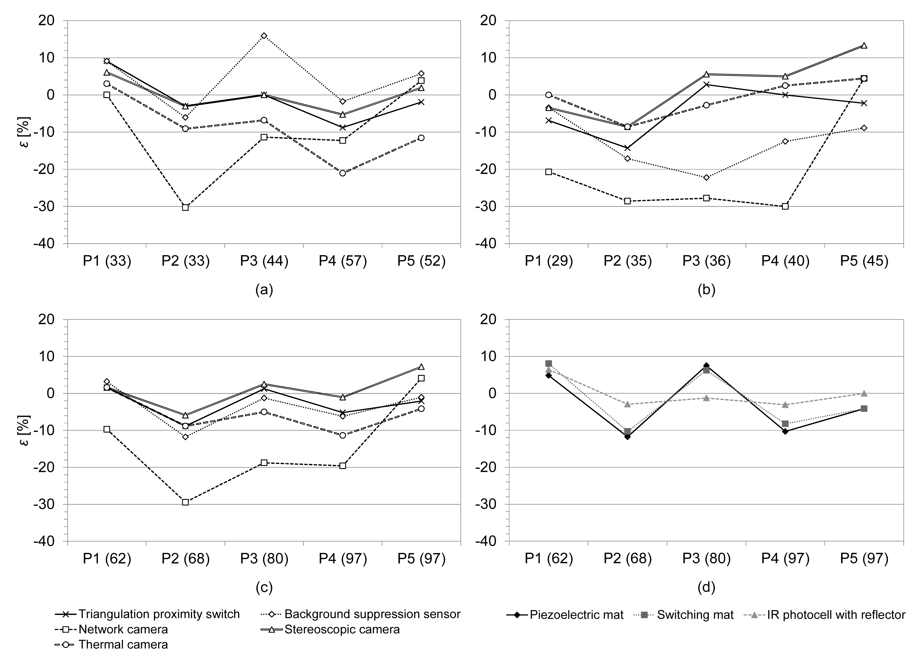
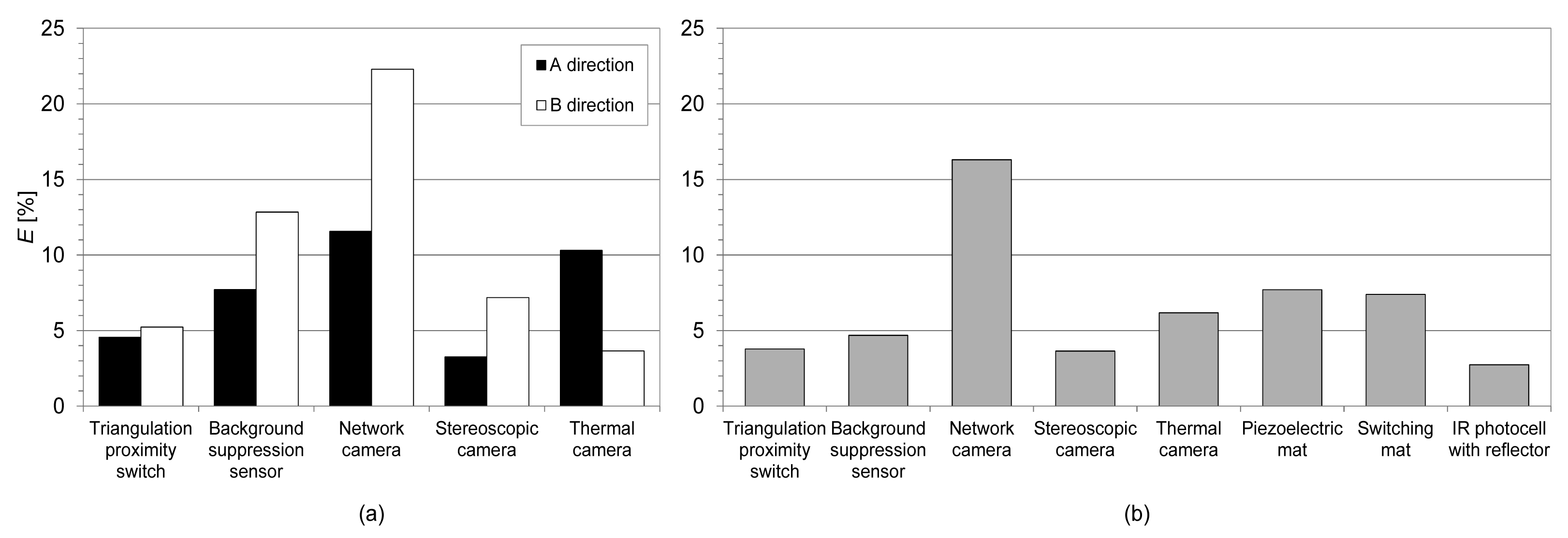
The hourly counting error rates of the sensor readings are presented in Figure 2 and the overall error rates in Figure 3. The mean overall errors in the A direction and in the B direction were 6.1% and 9.0% for the light beam sensors, and 8.4% and 11.1% for the camera sensors, respectively.

3.2. Relative Standard Deviations of the Sensor Readings

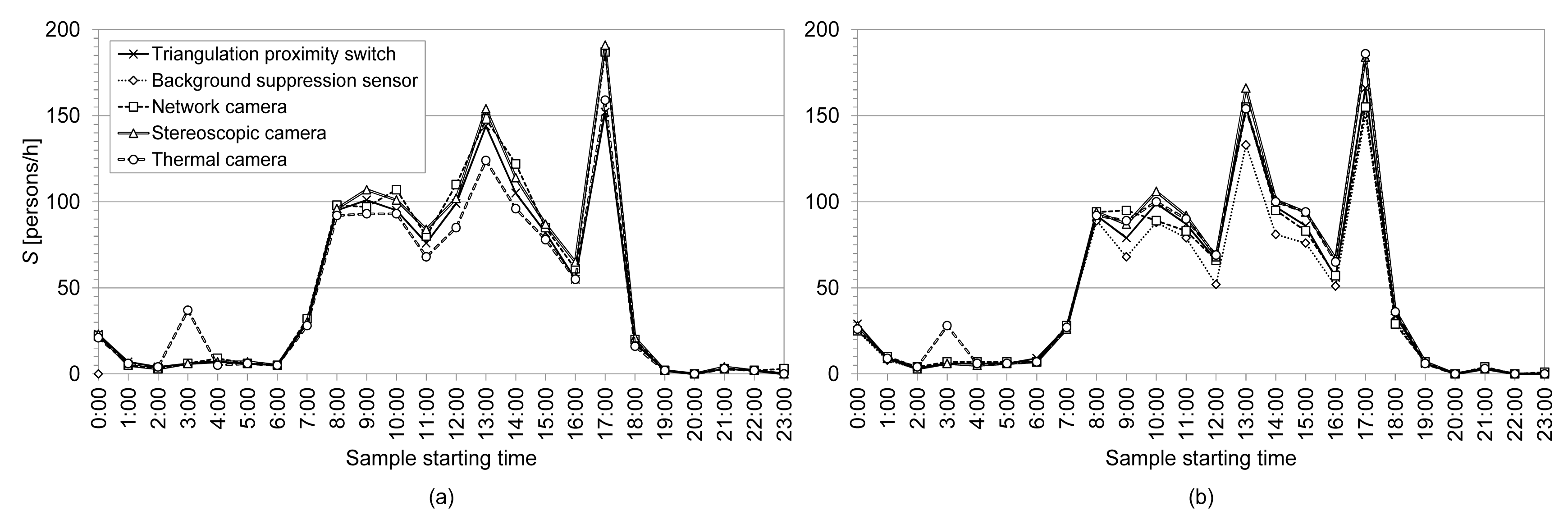
Different test sensors' average directional readings of the one-hour test samples were 0–169. To provide a picture of the expected results, an example one-day period of hourly sensor readings for both counting directions is presented in Figure 4. Some of the hourly samples were considered to involve a clear device malfunction and were discarded from the results. These included cases where only one of the sensors had a non-zero reading, or a reading that was ten times (or more) larger or smaller compared to the others. Samples of both directions were removed even if only one of the directions contained an error. The error always appeared in one sensor at a time and mostly to both directions simultaneously. Altogether 49 hourly samples out of 863 were discarded, leaving 814 samples of both counting directions for analysis. The number of samples discarded on account by sensor was: the network camera 29, the stereoscopic camera 5 and the thermal camera 15.

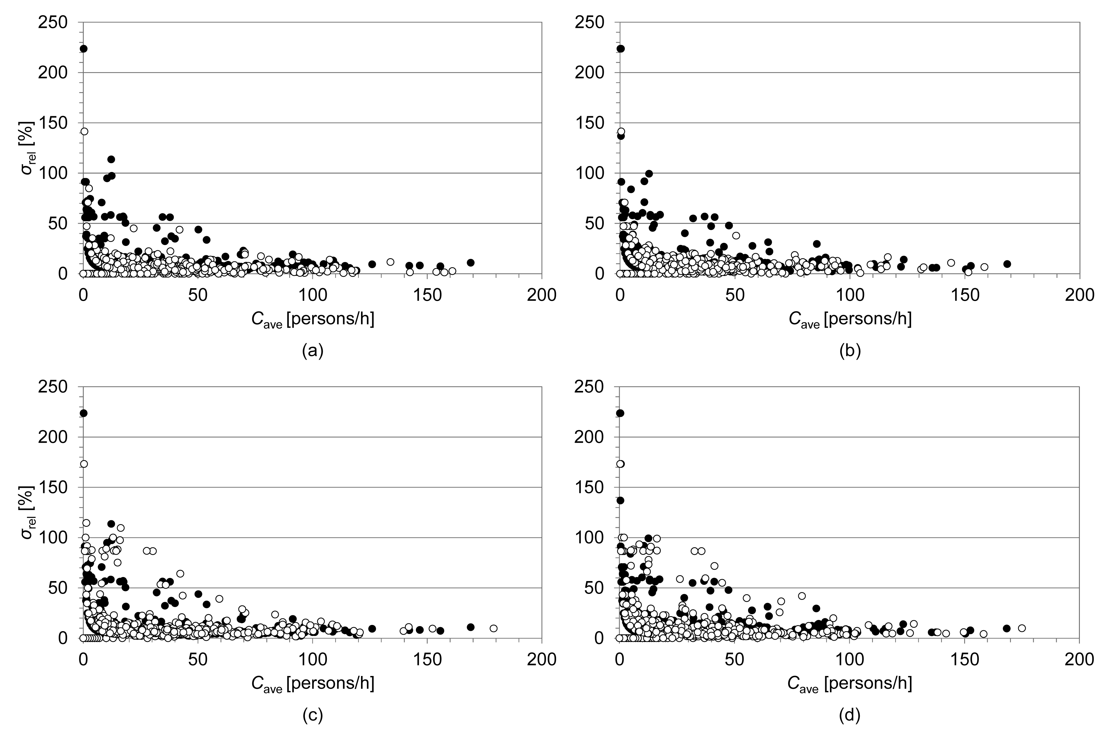
The relative standard deviation of the sensor readings in a certain group (Section 2.4.2) was plotted as a function of the corresponding average reading. Remarkable differences were found between the groups of different sensor technologies (3) and the group of all direction sensitive sensors (1). The results for these are presented in Figure 5.

3.3. Modeling of the Visitor Counting Sensor-Based DCV and CAV

Compared to the manual results, the triangulation proximity switch had low directional overall counting error rates (to the A direction 4.6% and to the B direction 5.2%), which were also the most equally balanced among all the sensors. Thus its results were used in modeling the DCV energy consumption. As the triangulation proximity switch generally tended to undercount (Figure 2), negative signs were added to the overall error rates used in the zone population calculations (Equations (4) and (5)).

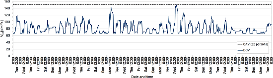
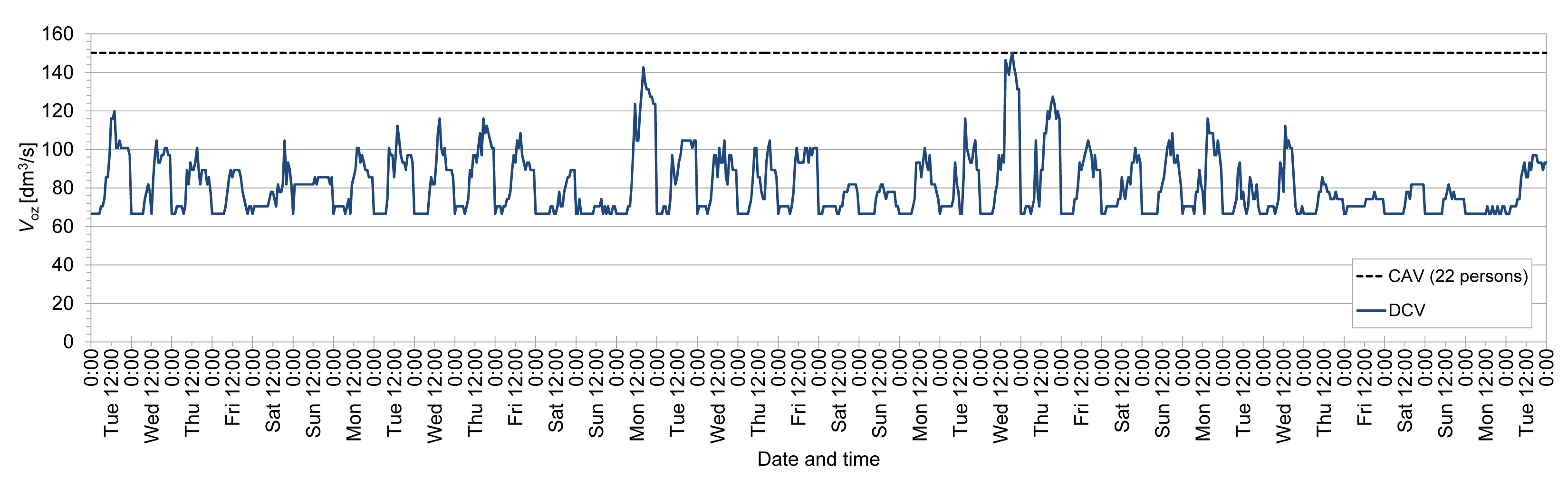
Based on the sensor data, the maximum zone population of the Café room was 22 persons, being also the time-weighted average of the zone population during the test period. The calculated hourly zone outdoor airflows of the visitor counting sensor-based DCV and the CAV with a setting point for the time-weighted average zone population (150.2 dm³/s) are presented in Figure 6. The mean, minimum and maximum values of total daily air volumes using visitor counting sensor-based DCV and CAV, the corresponding ratios of DCV and CAV and estimated daily savings in air transportation energy consumption and costs are presented in

Table 2. Characteristics of the comparison between the visitor counting sensor-based DCV and CAV. It was assumed that the ventilation system operated round the clock.

	Mean	Minimum	Maximum	SD a
Total air volume with CAV [m3/day]	12,977	12,977	12,977	0
Total air volume with DCV [m3/day]	6,999	5,823	8,695	675
DCV/CAV [%]	54	45	67	–
Energy saving [kWh/day] b	6.64	7.95	4.76	–
Money saving [EUR/day] c	0.99	1.18	0.71	–

^aStandard deviation of the daily readings;^bSaving in air transportation energy based on the specific fan power of 4.0 kW/(m³/s) with 100% outdoor air mode;^cBased on the price of 0.1485 EUR/kWh (average of available prices including electric energy, transmission and taxes) [30].

. At an annual level, the average savings with the modeled DCV strategy would be about 360 EUR a year, assuming that the hourly population levels in the Café remained approximately within the same order of magnitude through the year.

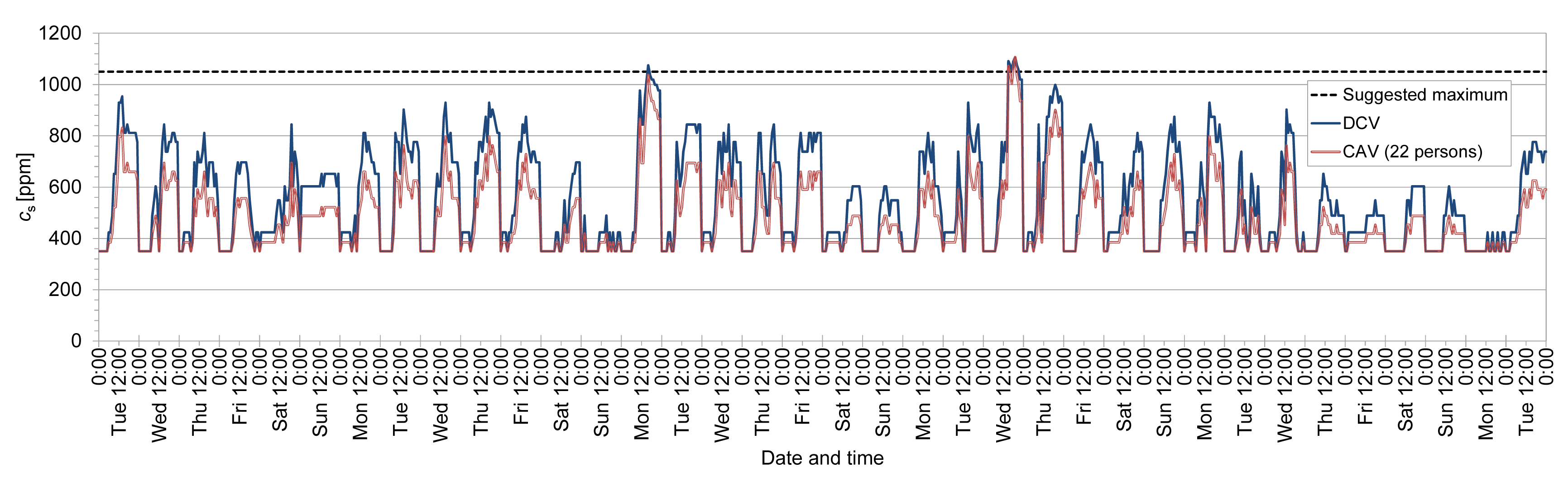
The calculated hourly steady state CO₂ concentrations in the Café with the modeled DCV and CAV are presented in Figure 7. The indoor CO₂ concentration was maintained within the limits of the estimated maximum concentration of a pleasant environment with sedentary persons occupying the space (1050 ppm) with the DCV in 99.1% and with the CAV in 99.7% of the hourly samples.

4. Discussion

4.1. Counting Performance of the Sensors

In the first part of this study multiple visitor counting sensor technologies were tested to find out the possible benefits provided by the more sophisticated camera sensors. The focus was on the five direction sensitive sensors that can be utilized in DCV.

All direction sensitive sensors have both positive and negative periodic counting errors (Figure 2). Compared to the manual results, the triangulation proximity switch has the most equally balanced directional overall counting error rates (4.6% and 5.2%), although the stereoscopic camera has a lower overall error in one direction (3.3% and 7.2%), Figure 3. Of the different direction sensitive sensor technologies, the light beam sensors have the lowest overall directional error rates. If the counting direction is ignored, the IR photocell with reflector has the lowest overall error (2.8%), implicating that the direction discrimination as such may cause some uncertainty in the counting results (Figure 3). Generally, the counting errors of the direction sensitive sensors increase and have more deviation when the counting directions are handled separately. This is due to the fact that directional over- and undercounting compensate each other when the direction is omitted.

Every direction sensitive sensor, except the thermal camera, has a larger overall error in the B direction than in the A direction. This is probably because of the different installation locations of the sensors. The thermal camera was mounted on the Café room side of the test site doorway, whereas the other counters were mounted on the corridor side (the background suppression sensor, network camera and stereoscopic camera) or at the doorway threshold (the triangulation proximity switch). As all sensors seemed to have more difficulties to accurately count people arriving from the opposite side of the doorway it was possible that the walls limiting the doorway in that case shadowed the sensors' fields of view. This is supported by the fact that the triangulation proximity switch, located at the doorway threshold, has the smallest difference between the two directional overall error rates.

The relative standard deviations of the sensor readings were analyzed based on the counting data of the whole 36-day period. The comparison of groups of all test sensors (1) and all test sensors with one sensor brand in turn removed (2) showed that omitting any single sensor had no remarkable effect on the result. The case was the same when comparing the deviations of one type of technology (3) and one type of technology with one sensor brand in turn removed (4). However, remarkable differences between different sensor technologies (3) could be seen when comparing them to the groups of all sensors (1), Figure 5. The light beam sensors seem to have smaller relative standard deviations than the camera sensors. However, in the A direction this is less obvious, and the reason is probably the different installation locations mentioned above. It should be also noted that hourly test samples had to be discarded only due to malfunction of the camera sensors.

The results also show that the relative standard deviation generally decreases as the average sensor reading increases (Figure 5). The average number of directional people flow samples of different volumes of all direction sensitive sensors is as follows: 350 (0–5 persons), 372 (6–50 persons), 92 (51–100 persons), 11 (101–150 persons) and 3 (150 persons or more). As the hourly people flow rates are concentrated in the lower volumes, it is also likely that there are more occasional erroneous readings among these samples. In the plots of the light beam sensors, the number of samples with a relative standard deviation of 50% or more is about 10, and in the plots of the camera sensors it is about 50 (Figure 5). As in the plots many of the markers overlap in the lower deviation values, the few higher values are overemphasized. Together with the fact that with low people flow volumes even small differences in the readings are significant, this is a possible reason why the ratio between average people flow and relative standard deviation seems to drop dramatically with the higher people flows.

The lower overall counting error rates and smaller deviations of the readings in the light beam sensors suggest that the insufficient installation height, moderate people flow rates and the pedestrian patterns occurring at the test site possibly did not do justice to the counting capabilities of the camera sensors. In light beam sensors, a misjudgment of the walking direction can occur if the two IR beams are cut in the wrong order. This can occur if pedestrians walk too closely after each other or arrive at the sensor simultaneously from opposite directions. Generally, the light beam sensors need to be installed high enough to avoid overcounting caused by swinging arms. In our test setup this was not a main concern as children very rarely visit the Aalto Design Factory building and the light beam sensors could be installed optimally to count grown-ups. The light beam sensors can detect only one person at a time and can miss detections if many persons pass them during too short an interval. Unfavorable environmental factors such as direct or flickering sunlight can cause video camera sensors to miss a person or cause ghost detections, whereas an infrared camera sensor is sensitive to airflows with temperature gradients. The camera sensors studied here have no absolute maximum number of persons that can be simultaneously counted in their field of view. Nevertheless, if the objects move too close to each other, they may not be separable and undercounting may occur.

Although the best possible test site was selected and the sensors were installed following the manufacturers' recommendations, the test location had some noteworthy defects that could have a negative impact on sensor counting performance. As every camera sensor needed to be installed in the middle of the monitored passage, they had to be placed back-to-back on both sides of the doorway. Thus all of them were in slightly different places along a line about 1.5 m long in the corridor direction. This could possibly cause problems in situations where a pedestrian turned back before they had been detected by every test device. Also the side-mounted light beam sensors were placed at different spots in the corridor direction. This was due to the fact that the background suppression sensor and triangulation proximity switch would interfere with each other if placed too closely. The doorway was also wide enough for multiple persons to walk through side-by-side. Although in observations this occurred relatively seldom, it was still a source of error in the counting results of the light beam and mat sensors.

Installation directly to the ceiling would have ensured the most optimal installation height for the camera sensors. The metallic air ducts on both sides of the doorway, however, would have blocked or limited their field of view, and thus mounting brackets were used to lower the cameras. As a result, the installation heights of all of them were reduced close to the recommended lower limits. Regardless of the brackets, it was found out that the air ducts caused reflections of the heat emitted by the passing persons, leading to ghost detections in the thermal camera. The problem had to be fixed by narrowing the width of its counting area in the configuration software. Painting the air ducts black in color would probably also have helped to reduce the reflections, but this was not permitted. The internal clock of the network camera's counting software was found out to drift during a couple of days, thus causing a dilemma in synchronizing it faithfully with the rest of the test sensors. Additionally, an irremovable emergency exit sign (visible in Figure 1) limited the network camera's field of view.

The widths of both mat sensors were slightly too small for the doorway. Hence passing them from the side was possible. The manufacturer of the switching mat sensor provided a mat larger in width but also in depth. Thus using it would have increased the possibility of overcounting. When monitoring the test site, it was also noticed that some of the passing people stepped over the mats, and a couple of them even intentionally walked back and forth in the sensor area, thus causing counting errors. Despite the fact that the digital indicators placed above the doorway provided a handy tool in verifying the sensor operation, they could also have attracted passers-by to uncontrolledly test the sensors.

4.2. Energy Saving Potential of the Visitor Counting Sensor-Based DCV

In the second part of this study the counting data of the most promising sensor, the triangulation proximity switch, was used to model air transportation energy consumption of a visitor counting sensor-based DCV. This was compared to the energy need of a modeled CAV with a ventilation rate set according to the time-weighted average of the calculated zone population of the Café room during the test period. Although nowadays the most common choice for public spaces is a CO₂ sensor-controlled DCV instead of a CAV, the comparison between the visitor counting sensor-based DCV and CAV provides useful theoretical information about the energy saving potential of the DCV.

As the people traffic through the second entrance (E2) of the Café had to be estimated based on the data of the sensor test site doorway (E1), the calculated hourly zone populations in this study are estimates as well. The results nevertheless suggest that there is plenty of room for energy savings in air transportation when using a visitor counting sensor-based DCV (Figure 6 and Table 2). The case-specific energy savings of a DCV naturally depend on the power consumption of the ventilation equipment used as well as the local price of electricity. Installing a DCV into an old building may also require significant investments in the existing ventilation system that should also be taken into account when modifications are considered.

Between the modeled DCV and CAV, there was no remarkable difference in the proportion of hourly samples where the Café room's calculated CO₂ concentration exceeded the estimated maximum concentration for a pleasant environment occupied by sedentary persons (1050 ppm). However, zone population detection with a one hour resolution can only be used to set the ventilation for the hour following the measurement. Thus it is possible that during the next hour the room occupancy will dramatically fall or leap, leading to over- or underventilation. Another possibility is to gather long-time occupancy history data that can be used to adjust the ventilation of rooms with predictable hourly zone populations. If the intention is to adjust the DCV in real time at least a minute-level resolution—realizable with a suitable data logger—is needed.

Although the CO₂ sensors may provide a more accurate determination of the current zone population than visitor counting sensors, the CO₂ measurement result may be misleading if the sensors are installed at inappropriate locations, such as in too high or low a position, or too far away from the zone occupants. For proper measurement results the CO₂ sensors should be located at the breathing air height of the room [4]. Another possibility is to place the sensors in the return air duct [8]. However, the fact that CO₂ concentrations seldom reach equilibrium in public buildings complicates the determination of the sufficient outdoor air flows [8].

Possible malfunctions in a visitor counting sensor-based DCV caused by sensor counting errors are related to the usually inevitable under- and overcounting. It is also possible that a visitor counting sensor of the DCV totally stops working for instance due to light beam drifting or crashing counting software. False or missing counting leads to erroneous determination of the zone population and too high or too low ventilation. In case a room has multiple entrances, more than one visitor counting sensor is needed. This inevitably causes an increase in the uncertainty of the occupancy determination. As the effect of the measurement error on the zone population calculation accumulate over time, it has to be taken into account when the minimum ventilation of the DCV-serviced zone is chosen and the threshold for a ventilation set point change is determined. If necessary, the design has to be done at the expense of energy consumption to always ensure an acceptable indoor air quality. Counting site-specific calibration of the visitor counting sensors is also advisable. Unnecessary ventilation in night-time can easily be prevented by turning the ventilation to the minimum setting point. For daytime use it would be reasonable to combine CO₂ sensors and presence detectors with the visitor counting sensor-based DCV. The visitor counting sensors will then enable a short response time in the ventilation control, while the other sensors can be used to confirm the airflow need. A drawback in this kind of sensor fusion, however, would be increased cost and complexity of the control system.

5. Conclusions

The study results suggest that the more sophisticated camera sensors do not bring any added value to the counting in the case studied here. It can be concluded that not all visitor counting sensors are suitable for all installation environments or all volumes of people flow. Instead, choosing a sensor should be based on the physical dimensions and the estimated overall people flow rate of the monitored passage. The suitability of the sensor in question should also be tested on the spot. Based on its good performance the triangulation proximity switch seems to be the most suitable one for the directional counting needed in DCV applications, as long as the visitor flow rates are moderate and people proceed mostly in a single file.

The comparison between different ventilation strategies suggests that significant savings in air transportation energy consumption could be gained by using a visitor counting sensor-based DCV instead of a CAV with a setting point based on the time-weighted average zone population of the room. However, for a virtually real-time control of ventilation, at least a minute-level counting resolution should be used. As the visitor counting sensors inevitably exhibit some counting error, counting site-specific calibration of the visitor counting sensors is advisable. A good solution could also be to equip the visitor counting sensor-based DCV with a backup control, such as a presence detector, to avoid unnecessary ventilation of the room during unoccupied periods. A DCV utilizing both visitor counting and CO₂ detection could be a possible solution to always guarantee sufficient ventilation with a short response time.

References

- Bauer, D.; Brändle, N.; Seer, S.; Ray, M.; Kitazawa, K. Measurement of Pedestrian Movements: A Comparative Study on Various Existing Systems. In Pedestrian Behavior; Timmermans, H., Ed.; Emerald Group Publishing Limited: Bingley, UK, 2009; pp. 325–344. [Google Scholar]
- Brown, S. Shopper circulation in a planned shopping centre. Int. J. Retail Distrib. Manag. 1991, 19, 17–24. [Google Scholar]
- Hashimoto, K.; Yoshinomoto, M.; Matsueda, S.; Morinaka, K.; Yoshiike, N. Development of people-counting system with human-information sensor using multi-element pyroelectric infrared array detector. Sens. Actuators A Phys. 1997, 58, 165–171. [Google Scholar]
- Mysen, M.; Berntsen, S.; Nafstad, P.; Schild, P.G. Occupancy density and benefits of demand-controlled ventilation in Norwegian primary schools. Energy Build. 2005, 37, 1234–1240. [Google Scholar]
- Emmerich, S.J.; Persily, A.K. Literature review on CO2-based demand-controlled ventilation. ASHRAE Trans. 1997, 103, 229–243. [Google Scholar]
- Hashimoto, K.; Kawaguchi, C.; Matsueda, S.; Morinaka, K.; Yoshiike, N. People-counting system using multisensing application. Sens. Actuators A Phys. 1998, 66, 50–55. [Google Scholar]
- Yoshiike, N.; Morinaka, K.; Hashimoto, K.; Kawaguri, M.; Tanaka, S. 360° direction type human information sensor. Sens. Actuators A Phys. 1999, 77, 199–208. [Google Scholar]
- Fisk, W.J.; de Almeida, A.T. Sensor-based demand-controlled ventilation: A review. Energy Build. 1998, 29, 35–45. [Google Scholar]
- Murphy, J.; Bradley, B. CO2-based demand-controlled ventilation with ASHRAE Standard 62.1-2004. Trane Eng. Newsl. 2005, 34, 1–8. [Google Scholar]
- Nassif, N. A robust CO2-based demand-controlled ventilation control strategy for multi-zone HVAC systems. Energy Build. 2012, 45, 72–81. [Google Scholar]
- Norbäck, D.; Nordström, K.; Zhao, Z. Carbon dioxide (CO2) demand-controlled ventilation in university computer classrooms and possible effects on headache, fatigue and perceived indoor environment: An intervention study. Int. Arch. Occup. Environ. Health 2013, 86, 199–209. [Google Scholar]
- Fan, Y.; Kameishi, K.; Onishi, S.; Ito, K. Field-based study on the energy-saving effects of CO2 demand controlled ventilation in an office with application of energy recovery ventilators. Energy Build. 2014, 68, 412–422. [Google Scholar]
- Benezeth, Y.; Laurent, H.; Emile, B.; Rosenberger, C. Towards a sensor for detecting human presence and characterizing activity. Energy Build. 2011, 43, 305–314. [Google Scholar]
- Naghiyev, E.; Gillott, M.; Wilson, R. Three unobtrusive domestic occupancy measurement technologies under qualitative review. Energy Build. 2014, 69, 507–514. [Google Scholar]
- Yang, F.; Ran, W.; Chen, T.; Luo, X. Investigation on the factors affecting the temperature in urban distribution substations and an energy-saving cooling strategy. Energies 2011, 4, 314–323. [Google Scholar]
- Zamora-Martínez, F.; Romeu, P.; Botella-Rocamora, P.; Pardo, J. Towards energy efficiency: Forecasting indoor temperature via multivariate analysis. Energies 2013, 6, 4639–4659. [Google Scholar]
- Yang, H.; Ozbay, K.; Bartin, B. Investigating the performance of automatic counting sensors for pedestrian traffic data collection. Proceedings of the 12th World Conference on Transport Research, Lisbon, Portugal, 11–15 July 2010.
- Bu, F.; Greene-Roesel, R.; Diogenes, M.C.; Ragland, D.R. Estimating Pedestrian Accident Exposure. Automated Pedestrian Counting Devices Report Available online: http://escholarship.org/uc/item/0p27154n (accessed on 5 January 2014).
- Bicycle and Pedestrian Detection. Available online: http://www.dot.state.mn.us/guidestar/2001_2005/nit2/Bike-Ped_Eval_Report-2-27-2003.pdf (accessed on 20 December 2013).
- Turner, S.; Middleton, D.; Longmire, R.; Brewer, M.; Eurek, R. Testing and Evaluation of Pedestrian Sensors. Available online: http://trid.trb.org/view.aspx?id=839627 (accessed on 10 December 2013).
- Bauer, D.; Ray, M.; Seer, S. Using Simple Sensors for Measuring Service Times and Counting Pedestrians: Strengths and Weaknesses. Proceedings of the Transportation Research Board 90th Annual Meeting, Washington, DC, USA, 23–27 January 2011.
- Kuutti, J.; Blomqvist, K.H.; Sepponen, R.E.; Kwak, J.; Kosonen, I. Performance of Commercial Over-Head Camera Sensors in Recognizing Patterns of Two and Three Persons: A Case Study. Proceedings of the 2013 IEEE Jordan Conference on of Applied Electrical Engineering and Computing Technologies, Amman, Jordan, 3–5 December 2013.
- Heikkilä, J.; Silvén, O. A real-time system for monitoring of cyclists and pedestrians. Image Vision Comput. 2004, 22, 563–570. [Google Scholar]
- Anberger, A.; Hinterberger, B. Visitor monitoring methods for managing public use pressures in the Danube Floodplains National Park, Austria. J. Nat. Conserv. 2003, 11, 260–267. [Google Scholar]
- Diógenes, M.C.; Greene-Roesel, R.; Arnold, L.S.; Ragland, D.R. Pedestrian Counting Methods at Intersections: A Comparative Study. Proceedings of the Transportation Research Board 86th Annual Meeting, Washington, DC, USA, 21–25 January 2007.
- Hutchins, J.; Ihler, A.; Smyth, P. Modeling Count Data from Multiple Sensors: A Building Occupancy Model. Proceedings of the 2nd IEEE International Workshop on Computational Advances in Multi-Sensor Adaptive Processing, Saint Thomas, VI, USA, 12–14 December 2007.
- ASHRAE Standard 62.1-2013, Ventilation for Acceptable Indoor Air Quality; American Society of Heating, Refrigerating, and Air-Conditioning Engineers, Inc.: Atlanta, GA, USA, 2013.
- Carnes, A. ASHRAE Standard 62—What Now? IAQ Design Overview. Available online: http://www.daytonashrae.org/downloads/presentations/ASHRAE_Dayton_62.pdf (accessed on 31 September 2013).
- Railio, J.; Mäkinen, P. Specific Fan Power—A Tool for Better Performance of Air Handling Systems. Proceedings of the 9th REHVA World Congress CLIMA 2007 WellBeing Indoors, Helsinki, Finland, 10–14 June 2007.
- Sähköenergian ja Siirron Hinnan Kehitys (Development of the Price of Electric Energy and Its Transmission in Finland). Available online: http://www.energiavirasto.fi/documents/10179/0/Hintojenkehitys.xlsx (accessed on 3 February 2014).