Economic Scheduling of Residential Plug-In (Hybrid) Electric Vehicle (PHEV) Charging


Abstract
: In the past decade, plug-in (hybrid) electric vehicles (PHEVs) have been widely proposed as a viable alternative to internal combustion vehicles to reduce fossil fuel emissions and dependence on petroleum. Off-peak vehicle charging is frequently proposed to reduce the stress on the electric power grid by shaping the load curve. Time of use (TOU) rates have been recommended to incentivize PHEV owners to shift their charging patterns. Many utilities are not currently equipped to provide real-time use rates to their customers, but can provide two or three staggered rate levels. To date, an analysis of the optimal number of levels and rate-duration of TOU rates for a given consumer demographic versus utility generation mix has not been performed. In this paper, we propose to use the U.S. National Household Travel Survey (NHTS) database as a basis to analyze typical PHEV energy requirements. We use Monte Carlo methods to model the uncertainty inherent in battery state-of-charge and trip duration. We conclude the paper with an analysis of a different TOU rate schedule proposed by a mix of U.S. utilities. We introduce a centralized scheduling strategy for PHEV charging using a genetic algorithm to accommodate the size and complexity of the optimization.1. Introduction
Increasing fuel prices, diminishing fossil fuel reserves, rising greenhouse gas emissions and political unrest have made plug-in (hybrid) vehicles an attractive alternative to traditional internal combustion engine vehicles (ICEV). The growth of plug-in (hybrid) electric vehicles (PHEVs) as a clean, safe and economical transportation option to ICEVs can be promoted by extending driving range, improving battery health and life, increasing electric grid reliability and promoting acceptance of PHEVs by the consumer. The degree of penetration of PHEVs as a transportation option depends on a variety of factors, including charging technology, communication security, advanced metering infrastructure (AMI), incentives to customers, electricity pricing structures and standardization. The wide-spread adoption of electric vehicles will have many multi-faceted socio-economic impacts. Among these are increased system load, leading to stressed distribution systems and insufficient generation, power quality and reliability problems, degrading battery health, scheduling of vehicles as a potential power source in an ancillary market, costs incurred versus revenues earned by end user in offering such services, along-with the dependence on variable consumer behavior have been considered as hurdles to PHEV implementation [1,2].
Insufficient battery state of charge has been cited as the primary consumer insecurity regarding PHEVs [3]. In this paper, we interpret this concern as the desire to have a fully-charged battery at the beginning of the daily commute. This consumer desire for daily full charge must be balanced against the desire on the part of the utility to shape its load curve and avoid a load spike due to concurrent vehicle charging. It is well-accepted that coordinated vehicle charging can be used to minimize the adverse effects of PHEVs on the electrical distribution grid [4,5]. Coordination can be either centralized or decentralized. A centralized strategy is one in which a central operator (or aggregator [6]) dictates precisely when every individual PHEV will charge, but may not be attractive to consumers who prefer to have complete authority over their transportation availability and/or electricity usage. Typically, the objective of such strategies is “valley-filling” in which the nighttime drop in load demand is decreased, resulting in a more level load profile. However, other objectives, such as system loss reduction, greenhouse emission reduction, battery lifetime extension, etc., can also be optimization factors [7–10]. A centralized control strategy will require a central repository that collects parameter information from all vehicles to provide an optimal charging profile. It has also been suggested that this might be taxing on communication channels and computation time [11]. However, we believe that a centralized solution is the preferred approach under current technological capabilities. Furthermore, since the control signal is sent by the aggregator, adaptation will be easier. Lastly, it can be contended that consumer confidence can be won through pricing incentives. Thus, in this paper, we expand on these earlier approaches and develop a centralized scheduling approach that balances the actual cost of generation, the levelized time of use rates and load demand.
Specifically, we propose an optimal approach to PHEV charging that:
provides full charging to the maximum number of vehicles;
shapes the load curve to avoid demand spikes and accomplish valley-filling;
minimizes the cost to the customer; and
uses the most economic forms of generation available.
The critical contribution is the selection of the most appropriate fitness function to optimally shape the load curve.
2. Background
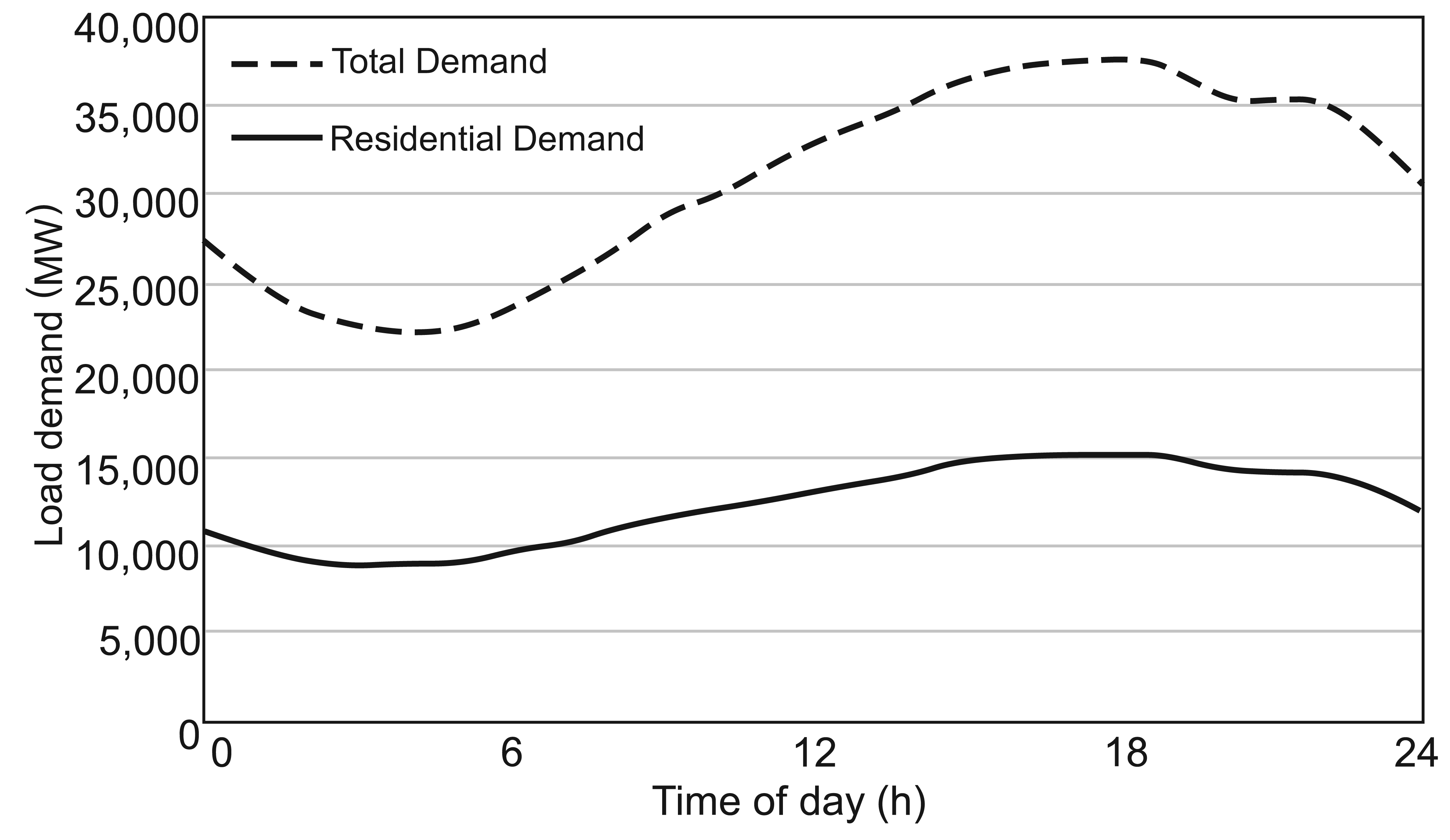
A regional load profile adapted from the California Independent System Operator (ISO) is shown in Figure 1. The top curve is a typical daily load demand; the lower trace is the associated residential load and is approximately 40% of the total demand. Each residential customer is assumed to have an average load of 4 kWh per day.
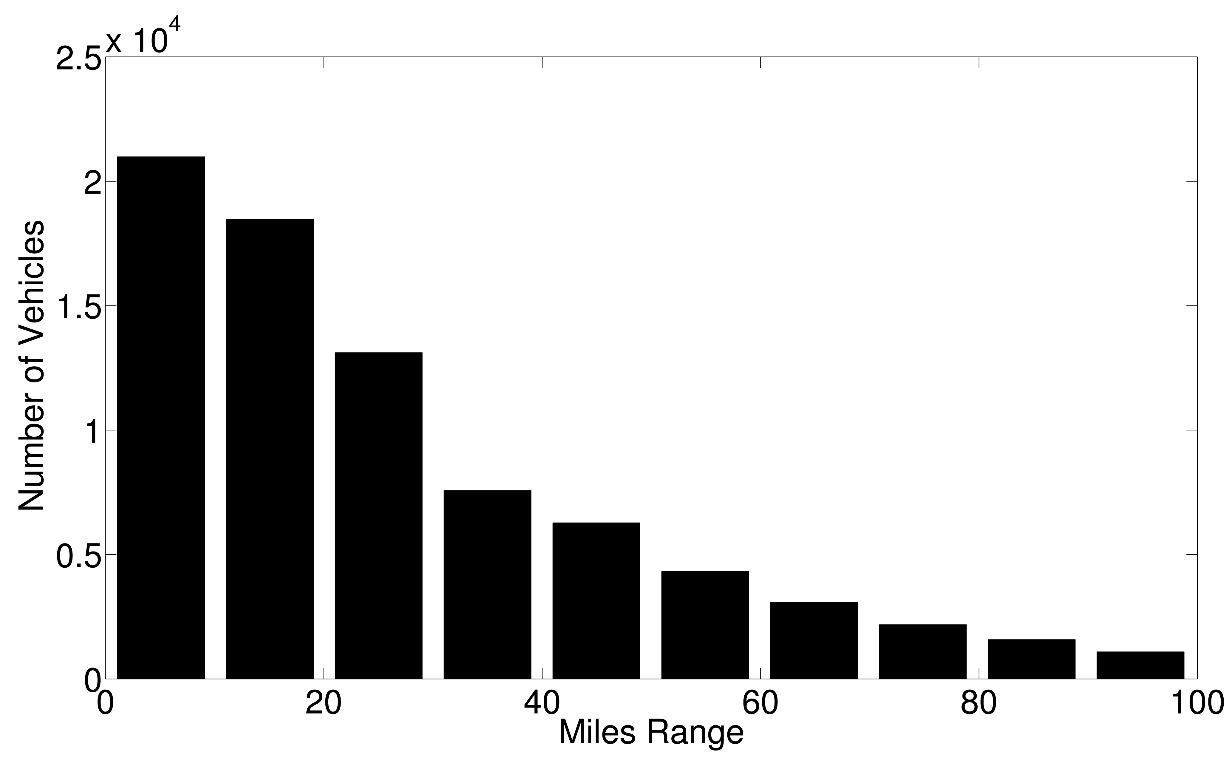
The 2009 U.S. National Household Travel Survey (NHTS) provides information regarding commuter behavior. The information pertinent to this paper is summarized in Figures 2 and 3.
The salient details from these data are that:
3. Process
Throughout the analysis presented, the following parameters were assigned randomly to each commuter, and the results presented are the average of a Monte Carlo-based simulation with 1000 trials:
battery size;
commute length;
return time;
time available before next trip;
charger type.
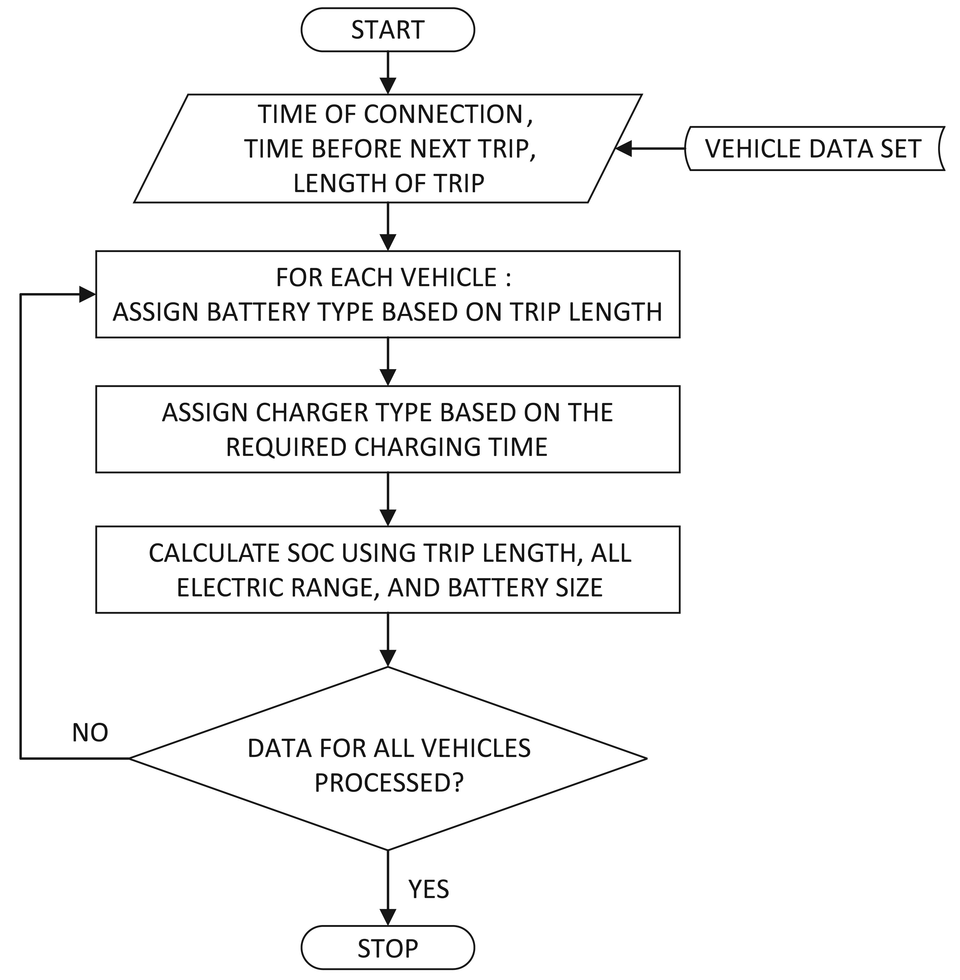
The commute length is randomly assigned to each household according to the distribution given in Figure 2. Based on the commute length, an appropriately-sized battery is then assigned.
Table 1 summarizes the batteries that are currently commercially available in the U.S. Based on these battery sizes, driver commute lengths (DCL) can be categorized and battery types associated, as shown in Table 2. Commuters in DCL20 are those that drive less than 20 mi daily, and their commute length can be adequately met by battery Types A–E, whereas a DCL100 commuter must have battery Type E.
Once the commute length and battery size have been assigned, then the return time is randomly assigned according to the distribution given in Figure 3. The time available before the next trip is also similarly assigned according to the distribution dictated by the NHTS. The chargers are assigned based on energy requirements. If the commute length and battery type require a Type II charger to fully charge, then a Type II charger is assigned; otherwise, a charger type is randomly assigned. The default assignment was generated by MATLAB, which uses Bernoulli-distributed random binary numbers and probability of zero parameter p = 0.5. Two types of chargers were used:
Type III chargers (480 VAC) have not been considered, because they are not intended for residential use. If the commute length, battery size and the time available before the next trip necessitated a Type II charger, then it was deterministically assigned; otherwise, the charger type was also randomly assigned.
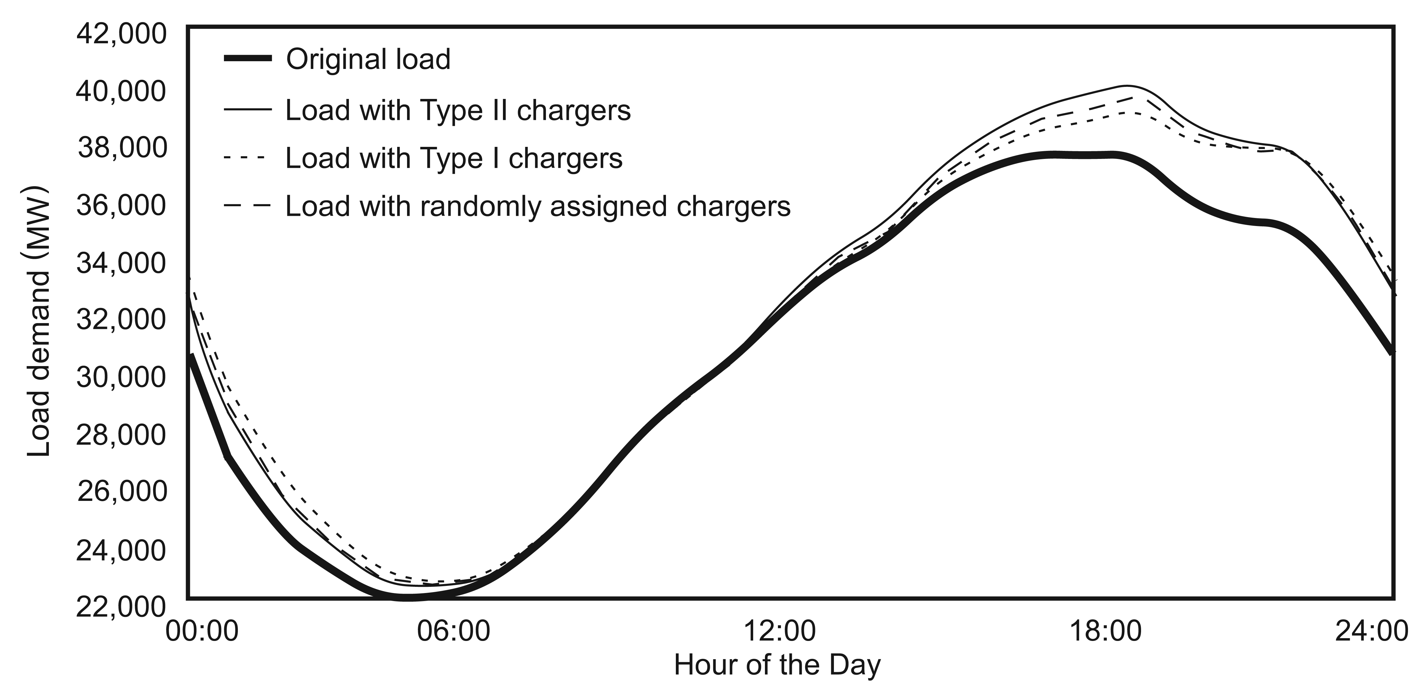
As a base case, this process was applied to the residential demand curve shown in Figure 1, and the average Monte Carlo simulation result (1000 trials) is shown in Figure 4. In this case, each commuter began the charging process immediately upon returning home. The base case residential load without any electric vehicle charging is shown as the bold trace. The load increases in all cases when there is electric vehicle charging. The worst case (highest peak) load occurs for Type II chargers. Since the Type II charger draws considerably more power than the Type I charger, the peak is higher immediately after the return home (around 18:00). However, since the vehicle batteries charged from Type II will more rapidly reach their full state of charge, the Type II load will more rapidly fall off during the valley period from 04:00 to 05:00. The Type I charger load is the lowest demand curve, and the randomly-assigned-charger load lies between the Type I and Type II curves. Battery charging characteristics play an important role in the maintenance and lifetime of the battery. However, it is not possible to capture these aspects in the model used, due to the differences in time scale. It is assumed that a typical charge cycle of bulk-absorb-float with the proper charger settings is used to avoid overcharging.
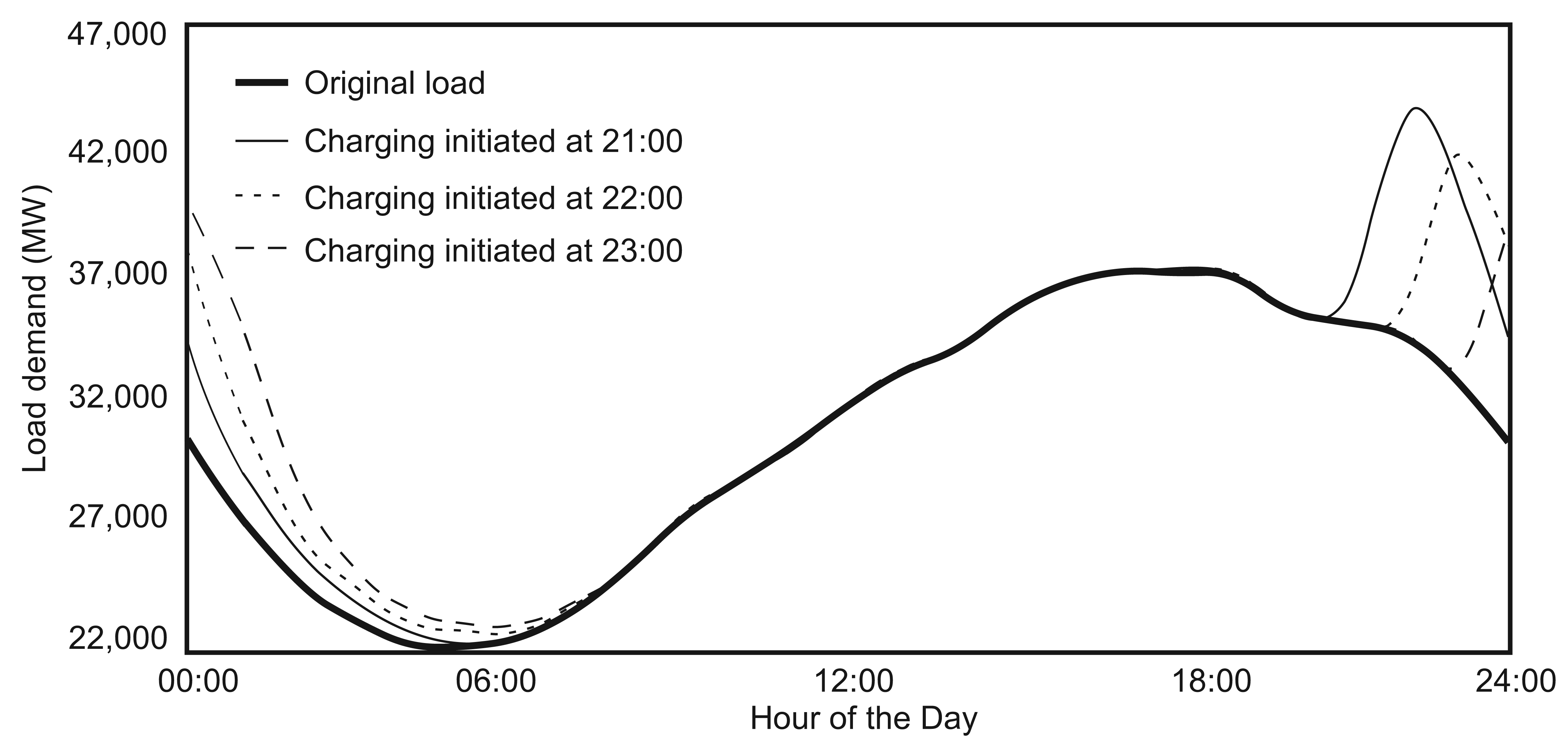
As a comparison to time of arrival charging, a delayed charger assignment was also considered. In these cases, the charger types are assigned randomly (in 1000 Monte Carlo trials) and the vehicles began charging at a set time (assuming they had already returned home). This is analogous to the situation of having off-peak pricing with 100% participation from commuters. This case is shown in Figure 5. Note that the resulting peak load is higher than in the variable charging initiation times, even though the charger type is assigned randomly. Obviously, a delayed charging scheme must be implemented with care.
4. Vehicle Aggregation
As noted previously, a centralized control scheme will most probably require the aggregation of the vehicles to reduce the complexity of calculating the charging schemes of multitudes of individual vehicles. The aggregation of vehicles is typically accomplished by grouping the vehicles according to common parameters, such as:
total charging time required (based on state of charge);
network topology and physical geography;
vehicle return time.
In this paper, we develop an aggregation scheme based on the total time required for charging, as illustrated in Figure 6. For simplicity, we also assume that the charging window is from 20:00 to 08:00, since the majority of vehicles are available for residential charging at this time. We assume that there are 12 possible connection times within the charging time frame (on the hour), but this can be expanded to any number of possible connection times without loss of generality (e.g., every 15 min), with added computational complexity. The vehicles are initially aggregated into equal sets that span the possible charging times. The illustration of the possible charging sets is shown in Figure 7.
Each possible charging set is called a “bin”: there are twelve one-hour charging bins, eleven two-hour charging bins, etc., and only one twelve hour charging bin. The charging times are based on the randomly assigned vehicle travel data from the NHTS, which specifies the respective anticipated state of charge for each vehicle. It is assumed that once a vehicle starts charging, it will remain charging until it is fully charged (i.e., no disconnect and reconnect). The required charging time for each vehicle in the study set is calculated. The number of vehicles requiring each length of charge time is shown in Figure 8. Because the majority of drivers have a commute length less than 30 mi, there is a large number of vehicles requiring only 1–5 h of charging (based on battery type and charger type).
Once the vehicles have been assigned to their initial charging set, then the energy required for each charging set is calculated. The total energy required at each hour is the summation of all charging sets in that hour. A genetic algorithm is then used to assign the charging sets to the optimal connection times. In the genetic algorithm, each chromosome in the population represents a particular charging scheme in which each of the chromosome's genes represents the number of vehicles in the charging set. A fitness function is used to specify which chromosomes are retained in each generation. As the generations progress, the algorithm will reallocate the charging sets from Figure 7 across the time spectrum to optimize a given fitness function. Figure 9 describes the optimization process. The choice of fitness function can significantly impact the resulting load profile. As an example, a simple fitness function is chosen:
Several different fitness functions are summarized in Table 3. The fitness functions are described:
The absolute difference between the system load and the projected average load is minimized.
The squared difference between the system load and the projected average load is minimized.
The plug-in time for each vehicle is delayed as long as possible based on vehicle state of charge (SOC).
Total cost is minimized (described later).
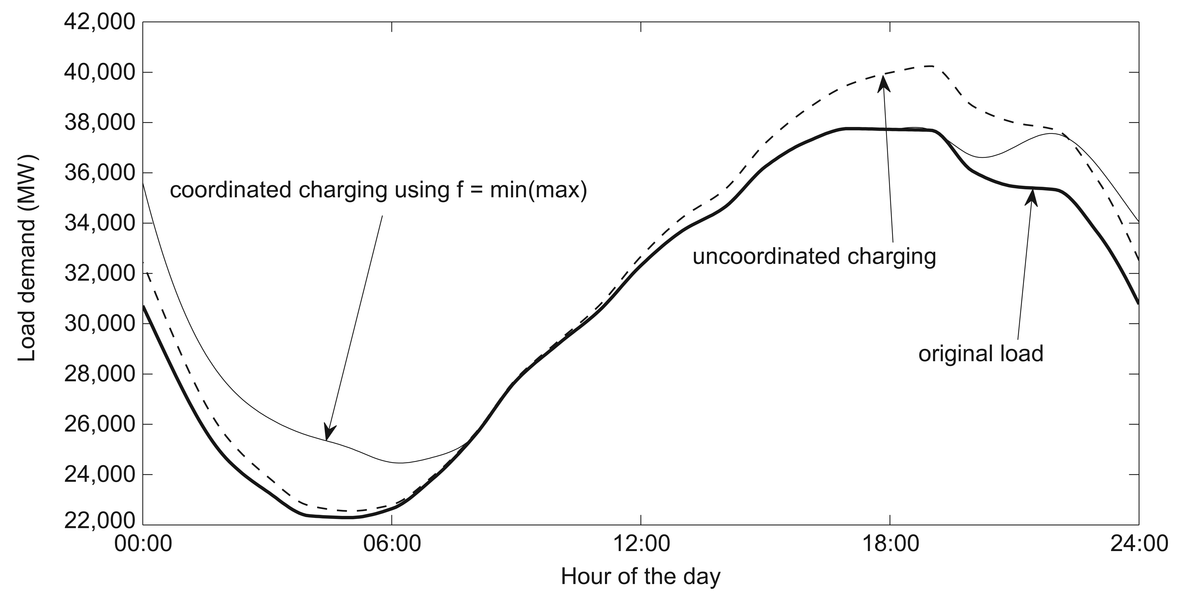
Figures 11 and 12 show the optimization results for the algorithms in Table 3. Note that there is not one “best” algorithm. Each charging profile is optimal for the fitness function for which it was defined, but the notion of “best” depends on the user. For example, Profile (A) strives to minimize the absolute error between the total load and a pre-determined average. From the results shown in Figure 11, Profile (A) decreases more or less monotonically throughout the charging period. Similarly, Profile (B) minimizes the squared error between the total load and a pre-determined average. This results in a relatively flat load profile. The drawback to Algorithms (A) and (B) is that the algorithms require an estimate of an average load. This may not be feasible if the overall load profile is changing rapidly. The min-max algorithm initially presented was not pursued further, because it performed poorly when compared with the algorithms presented in Table 3. The min-max algorithm considers only the maximum load for a day, which does not capture the complete behavior of the system during off-peak hours. The other fitness functions use a collective system behavior rather than a point behavior to address the problem of load scheduling. The system cost provides for a better fitness function that is capable of giving better results along with a well justified objective for any real-world problem.
Profile (C) assigns vehicle charging as late in the charging window as possible and, therefore, skews all of the load towards 8:00 am. Obviously, this approach is not “optimal” in terms of practicality, since this causes a second (but lower) peak in earlier morning which, leads to difficult load following by generation.
One or more of these algorithms may not be considered suitable for practical implementation. Every utility or aggregator may have their own notion of an optimal practical profile. One obvious approach is to optimize vehicle charging based on cost, but cost is not necessarily a straightforward function. The cost to the customer is not necessarily the cost to the utility. Customers typically want to minimize their cost of electricity, whereas utilities want to maximize their profits.
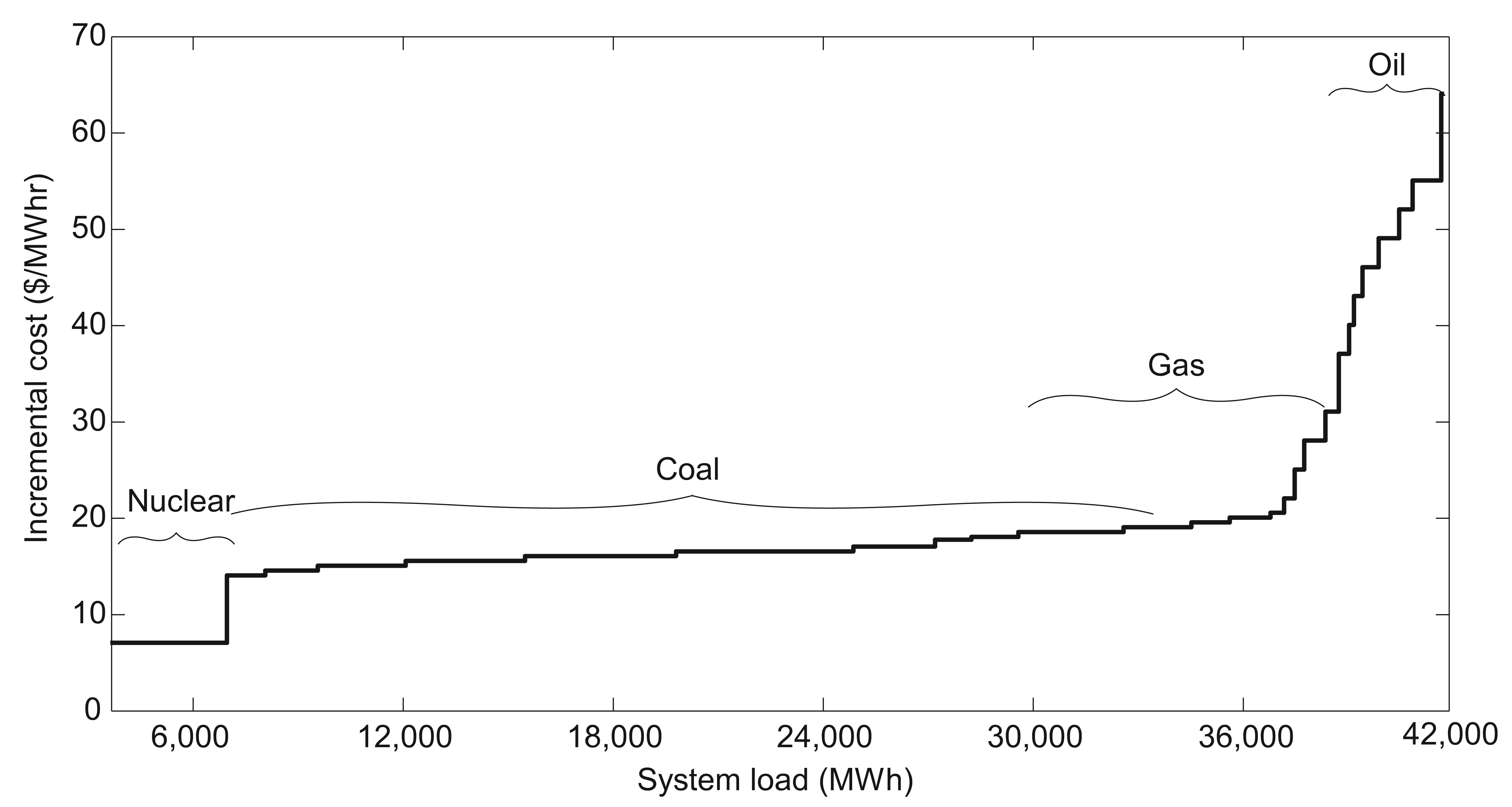
To better understand the impact of vehicle charging loads on utility cost, the set of incremental costs shown in Figure 13 are applied to the load profile. These incremental costs have been scaled and adapted from [13]. The horizontal lines indicate the incremental costs that are superimposed on the load profiles in Figure 14. The optimization algorithm is then used to identify a vehicle charging profile that minimizes the overall cost of generation during the charging window. These results are indicated as Profile (4) in Figures 11 and 12. This approach moves the vehicle charging away from the peak load, but since the incremental cost is constant between 24,000 and 26,000 MWh, there is not a significant shifting of load during the valley period. The minimum cost profile is very similar to Profile (B), which is the minimum squared error. Therefore, Algorithm (B) could be used as a computationally efficient approximation for finding the minimum cost. Algorithm (D) is the most computationally-intensive method, because it requires that the cost be evaluated for every chromosome at every iteration. The other fitness functions only require the actual power resulting from the chromosome. Table 4 summarizes the costs of the different algorithms with respect to the base load over the eight-hour charging period.
5. Time of Use Rates
The load shapes presented in the preceding section were developed to minimize the impact on the utility system. There is, however, currently little or no incentive for vehicle owners to allow the utility to control their charging times to produce these optimized load shapes, since they are not typically charged real-time prices that correspond to the actual load. In fact, the most probable situation is one in which the owners start charging their vehicles immediately upon returning home (which results in the uncoordinated charging profile of Figure 4). Many utilities have considered implementing a tiered time of use (TOU) structure to encourage owners to defer charging to non-peak times.
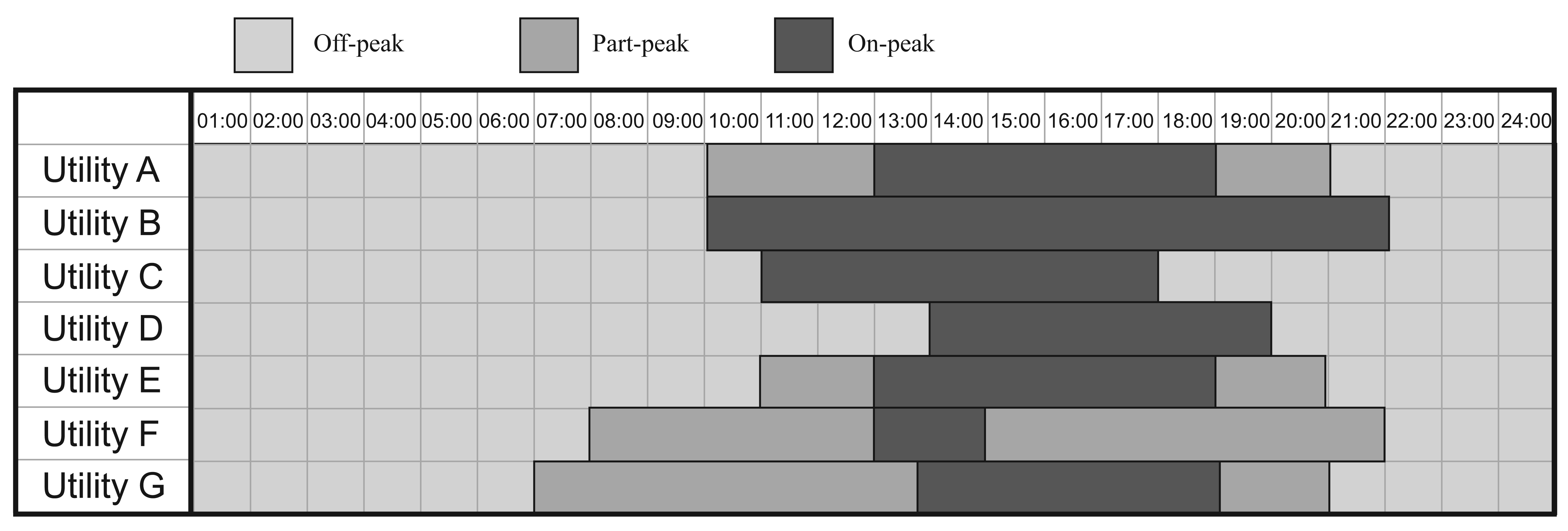
Utilities across the U.S. have adopted different time of use rates to incentivize customers to better manage their energy use. Most TOU rates are two (on-peak and off-peak) or three different rates (on-peak, part-peak, off-peak). Figure 15 shows the TOU rates for several U.S. utilities, and Table 5 gives representative rates [14–20].
To compare the impact of the various charging profiles on the cost to the customer, these cost structures are applied to the load profiles of the various charging algorithms and plotted in Figure 16. These rate structures are used for example purposes only; it should be noted that the actual cost per kilowatt hour for each utility may be different than the rates given in Table 5. An analysis of Figure 16 yields several trends. Utility B is the most expensive, since their on-peak rates are the longest. Utility D has the shortest on-peak hours, but is more expensive than Utility C and Utility E, because the on-peak rates extend later into the evening and pick up the large load. Utility G is also relatively expensive, because their off-peak rates are the shortest and their partial peak hours start at 07:00 hours.
6. Algorithm Integrity
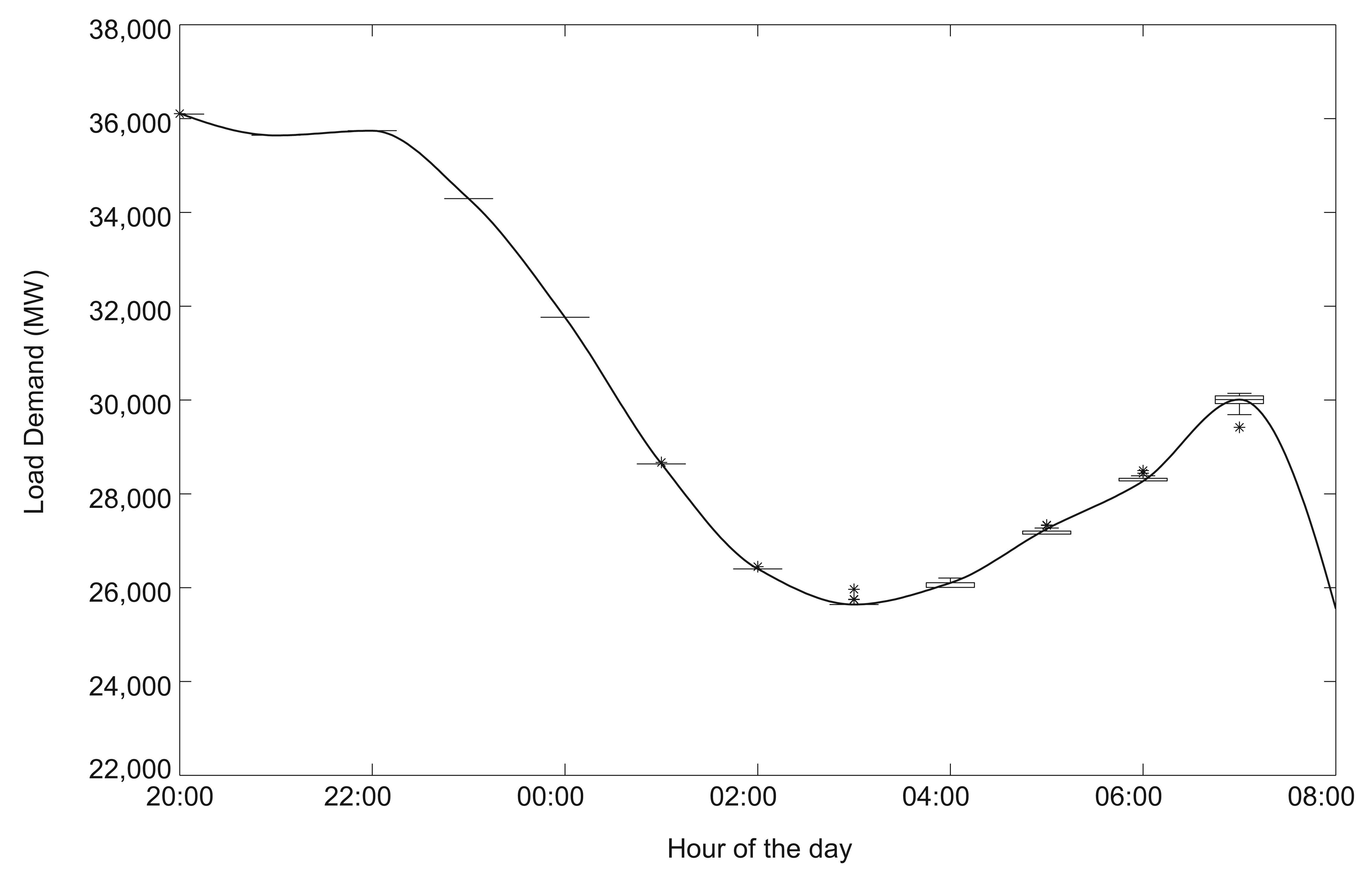
To test the integrity of the optimization algorithm, several benchmarks were analyzed. Since at the heart of the algorithm is a random assignment of vehicles, a metric was needed to measure the possible deviation in results and their impact on the load profiles. To measure the statistical deviation, the algorithm was run 50 times using Algorithm (C). The cumulative results are shown in Figure 17. The horizontal line represents the mean value of the data. The rectangles (when included) give the 25% and 75% percentiles with the upper and lower bars giving the maximum and minimum values. The stars (*) indicate statistical outliers. Note that at the beginning of the charging interval, the load values across all runs are tightly coupled. This is due to lack of flexibility in scheduling the long charge/low state-of-charge vehicles. However, as the charging window progresses, there is more possibilities for scheduling the one- and two-hour charging vehicles; thus, there is greater deviation. However, even considering the spread of values obtained, the load shape still remains relatively consistent; thus, the algorithm produces statistically similar results from run to run. This validates the optimization approach and algorithm.
Another method of testing algorithm integrity is to apply it to other load profiles. Figures 18 and 19 are two seasonal profiles adapted from ERCOT (Electric Reliability Council of Texas). Figure 18 represents a typical work day in January, and Figure 19 represents a typical work day in June. The January profile is similar to the California ISO (CAISO) load profile, but with a higher load factor (the ratio of the average load to the maximum load). The charging profiles are qualitatively similar to those obtained in Figure 11. As with the CAISO load profile, Algorithm (C) (scheduling charging as late as possible in the charging window) gives poor results and, in this case, actually causes an early morning peak. Algorithm (D) (minimum cost) once again provides the best outcome, but still results in a second, late evening peak. One possible method of improving the load characteristics is to allow charging to start earlier (at 17:00 instead of 20:00, as is currently used). The ERCOT June profile is quite interesting. The demand factor is very high; therefore, there is little valley to “fill”, nor is the cost differential between minimum and maximum significant. The minimum cost algorithm still provides the best results, but the resulting charging load is still unwieldy. In this case, a different charging policy would serve the ERCOT region better, such as providing charging access during the day at places of employment, shopping centers, parking garages, etc.
7. Test System Formulation and Algorithm Application
The coordination scheme is applied to a test system, and the results are thus quantified by means of load profile and voltage variations of the system.
7.1. System Specification
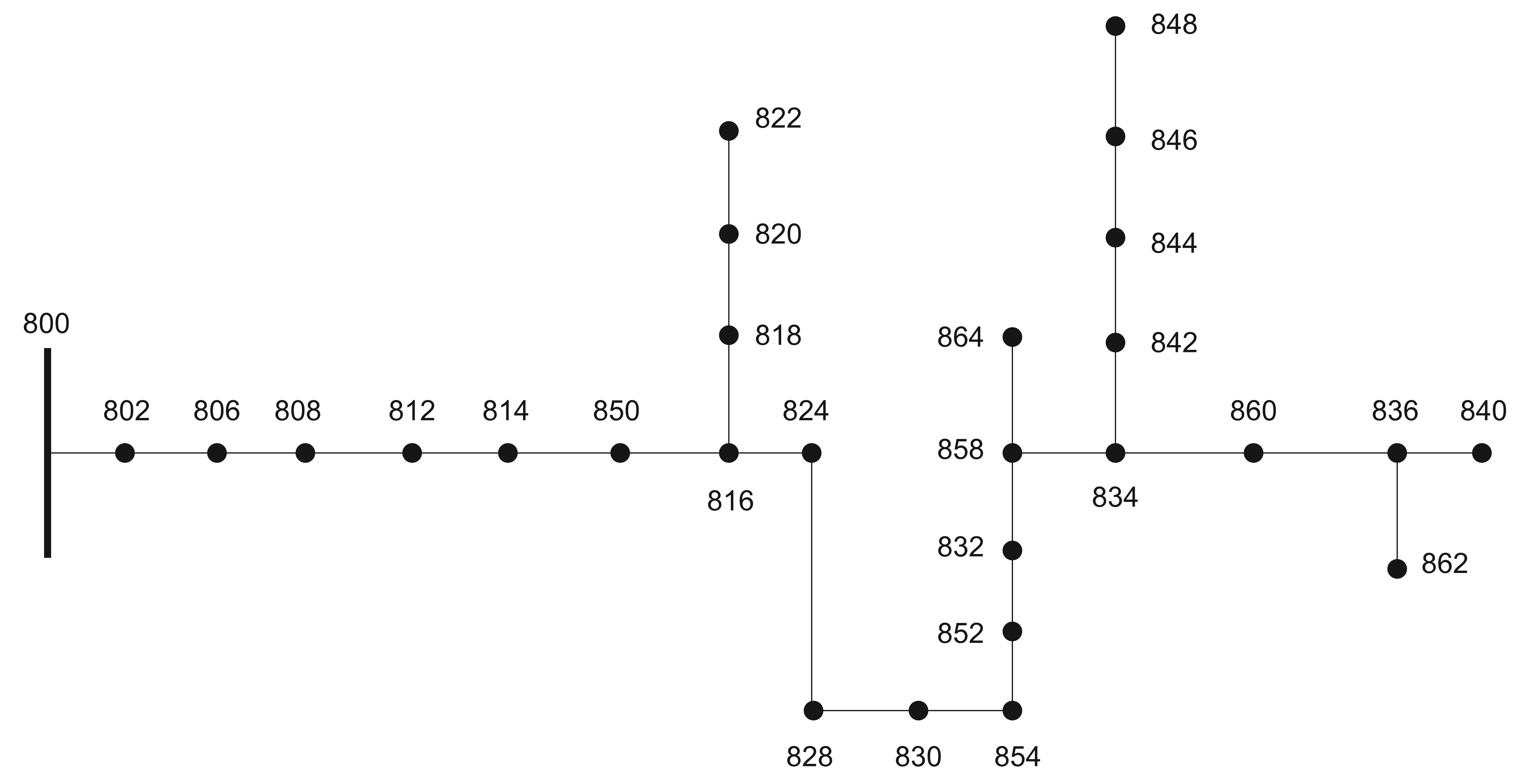
A three-phase balanced system, modified from the Institute of Electrical and Electronics Engineers (IEEE) 34 bus system [21], was formulated to test the impact of the algorithm (Figure 20). A daily load profile for the test system and also for the individual nodes was made to match the initial load profile studied. The approximate number of houses at each node was calculated assuming 4 kW of maximum load per house. Considering one electric vehicle per household as a 100% penetration on the system for the worst case scenario, the number of vehicles equals the number of houses at each node.
7.2. Vehicle Load on the Test System
A total of 147 houses, and, thus, vehicles, were selected for the test system. A set of vehicles was randomly selected from the NHTS dataset, which were randomly assigned to 11 nodes. Only eleven nodes of the test system had loads. The total number of houses on the system is 147. Since 100% penetration of vehicles is considered, each house is assigned one electric vehicle randomly from a pool of vehicles selected from the NHTS database. The vehicles are distributed in proportion to the load at each node. The vehicles were selected in the same ratio as in the NHTS database with regards to the time required for charging. This selection is attributed to the general driving patterns from the NHTS database. Once assigned to a node, it is assumed that the vehicle load would be observed at the same node, which is representative of the ownership of a vehicle and Type I charging at home.
7.3. Load Profiles
Having obtained the vehicle characteristics at each node, three other profiles were obtained, namely:
Load under uncoordinated vehicle connection: The vehicles are connected whenever the driver arrives home. Charging is completely under the control of the customer.
Load under global coordinated vehicle connection: The vehicles are assigned charging times between 20:00 and 08:00, depending on the SOC of the battery. The control is at the substation (Node 800), which coordinates all the 147 vehicles together.
Load under local coordinated vehicle connection: This is very similar to the global scheme with the exception that each node uses its respective load profile to coordinate the vehicles connected to that node.
The coordination schemes were run 50 times each, in order to obtain a range of load profiles.
7.4. Fitness Function
Minimizing the total sum of the deviation of instantaneous load from the average residential load was used as the optimization objective. It was found that this average value when varied over a range gives slight changes in the profile. The Pavg of the total load profile (residential + vehicle) gives better results than the Pavg of the residential load profile alone. This signifies the importance of the prediction of the vehicle load in the efficacy of the algorithm.
7.5. Results for the Test System
The load (Figure 21) and voltage profiles (Figure 22) show significant improvement from the uncoordinated profiles. The high voltage in the uncoordinated case during hours 01:00–08:00 is due to fewer loads on the system. The global and local load profiles give similar load profiles. These profiles are similar for all nodes in the system.
In addition to differences in load, the impact on feeder voltage is also an important consideration. It can be observed in Figure 23 that uncoordinated charging leads to large deviations in voltages, but global and local coordination results in far less deviation in voltage.
The analysis of variance (ANOVA) on the deviation of the daily voltage shows that the coordinated cases have a total deviation much lower than the deviation obtained for the uncoordinated case and are, thus, a better choice of coordination scheme. Figure 24 shows the mean deviation of daily voltage in case the coordinated load is less than that for the residential and the uncoordinated load profile cases. The voltage variation at each node for the coordination schemes (100 runs) is also shown in the box plot in Figure 25. The nodes closer to the substation (Node 800) show far less variation than the nodes further along the feeder.
Given that voltages were obtained from 50 runs each of global and local coordination schemes, a probability density function (pdf) of the voltage variation along with a box plot was obtained for each node. The pdf at each node is similar to that obtained for node 840 (Figure 26). This gives us a range within which voltage at that node will vary given the vehicle set connected according to either the local or global coordination schemes. The x-axis gives the node voltage and the y-axis indicates the percentage of time that particular voltage was obtained.
The improvement and minimal deviation in voltage is the motivation behind the application of the algorithm for vehicle connection.
8. Global versus Local Coordination
The global and local schemes differ in decision-making policies with regards to responsibility and authority. The global scheme works with a central authority that makes the decision for the system, given the system condition. The local scheduling scheme provides greater autonomy to the nodes to handle their individual loads, hence a decentralized responsibility structure and a probable less overhead on the central unit. The idea behind global optimization is to use the complete system information, while the local scheme uses the local load profiles and information specific to the respective nodes. The lack of system information might lead to erroneous results in case of faults or unforeseen load deviations that might change the shape of the local load profiles, which are the basis of the proposed optimization schemes. The global scheme might turn out to be more resilient in such situations. Communication is much higher in the case of a global scheme than in that of a local scheme. Each node sends a ‘tuple’ of information to the central unit, which is then processed at the central unit, and the resulting control signals are sent back to the nodes for optimal scheduling. The local scheme, on the other hand, makes decisions using the local information, thus reducing the communication overhead. Here, the increased cost of communication in the case of the global scheme would have to be compared with that of the installation cost of the smart control capability at each node in the case of the local scheme. Secure transfer of information is also of crucial importance in either scheme, which would incur extra costs.
Given the pros and cons of either scheme, different structural and functional decision policies can be proposed:
A hybrid, two-tiered structure can be implemented, where the authority and the responsibilities can be shared at the global and local levels. Probably, a local optimal scenario can be generated and sent to the central unit, which can then finally approve the schedule in view of the system condition. In case of a communication break between any node and the central unit, the local scheme can be implemented at the node.
The local structure proposed in the paper provides complete autonomy to the nodes in a complete non-cooperative environment. A cooperative scheme can be discussed wherein the neighboring nodes share local information and cooperatively decide on their scheduling schemes. This would be classified as a cooperative decentralized scheme.
A distributed scheme can also be implemented, where the central authority designates the responsibility of scheduling to the nodes. This can be done in a cooperative or non-cooperative manner at the nodes. A cooperative dynamic structure might be the best fit in a real-time scenario.
The above discussion is focused on static scheduling schemes. Dynamic scheduling or real-time scheduling would be the next step in this direction, due to the additional complexities of individual driving patterns.
9. Conclusions
This paper describes an aggregation method that can be used for scheduling plug-in vehicles for charging. A series of fitness functions are proposed and tested to illustrate the effect of different charging schemes on the total load as a function of charging load. Time-of-use rates are also analyzed to indicate which scenarios lead to the least customer and utility cost. Better voltage profiles and lower voltage deviations were obtained for the test system, followed by ANOVA analysis, showing the effectiveness of the coordination scheme. Future work will consider different charging policies, different rate structures and load demand profiles.
Acknowledgments
The authors gratefully acknowledge the financial support of the National Science Foundation under projects EFRI-0835995 and ECCS-1068996.
Conflicts of Interest
The authors declare no conflict of interest.
References
- Fernandez, L.P.; Roman, T.G.S.; Cossent, R.; Domingo, C.M.; Frias, P. Assessment of the impact of plug-in electric vehicles on distribution networks. IEEE Trans. Power Syst. 2011, 26, 206–213. [Google Scholar]
- Dyke, K.J.; Schofield, N.; Barnes, M. The impact of transport electrification on electrical networks. IEEE Trans. Ind. Electron. 2010, 57, 3917–3926. [Google Scholar]
- Egbue, O.; Long, S. Barriers to widespread adoption of electric vehicles: An analysis of consumer attitudes and perceptions. Energy Policy 2012, 48, 717–729. [Google Scholar]
- Morrow, K.; Karner, D.; Francfort, J. Plug-in Hybrid Electric Vehicle Charging Infrastructure Review; Final Report INL/EXT-08-15058; Idaho National Laboratory: Idaho Falls, ID, USA; November; 2008. [Google Scholar]
- Stroehle, P.; Becher, S.; Lamparter, S.; Schuller, A.; Weinhardt, C. The impact of charging strategies for electric vehicles on power distribution networks. Proceedings of the 8th International Conference on the European Energy Market, Zagreb, Croatia, 25–27 May 2011; pp. 51–56.
- Callaway, D.S.; Hiskens, I.A. Achieving controllability of electric loads. IEEE Proc. 2011, 99, 184–199. [Google Scholar]
- Sortomme, E.; Hindi, M.M.; MacPherson, S.D.J.; Venkata, S.S. Coordinated charging of plug-in hybrid electric vehicles to minimize distribution system losses. IEEE Trans. Smart Grid 2011, 2, 198–205. [Google Scholar]
- Acha, S.; Green, T.C.; Shah, N. Effects of optimised plug-in hybrid vehicle charging strategies on electric distribution network losses. Proceedings of the IEEE PES Transmission and Distribution Conference and Exposition, New Orleans, LA, USA, 19–22 April 2010; pp. 1–6.
- Deilami, S.; Masoum, A.S.; Moses, P.S.; Masoum, M.A.S. Real-time coordination of plug-in electric vehicle charging in smart grids to minimize power losses and improve voltage profile. IEEE Trans. Smart Grid 2011, 2, 456–467. [Google Scholar]
- Bashash, S.; Moura, S.J.; Forman, J.C.; Fathy, H.K. Plug-in hybrid electric vehicle charge pattern optimization for energy cost and battery longevity. J. Power Sources 2011, 196, 541–549. [Google Scholar]
- Gan, L.; Topcu, U.; Low, S. Optimal decentralized protocol for electric vehicle charging. Proceedings of the 50th IEEE Conference on Decision and Control and European Control Conference, Orlando, FL, USA, 12–15 December 2011; pp. 5798–5804.
- 2009 National Household Travel Survey. Available online: http://nhts.ornl.gov (accessed on 5 May 2011).
- Crow, M.L. Computational Methods for Electric Power Systems, 2nd ed.; CRC: Boca Raton, FL, USA, 2010. [Google Scholar]
- Pacific Gas and Electric Company. Available online: http://www.pge.com/mybusiness/energysavingsrebates/timevaryingpricing/timeofusepricing/ (accessed on 10 August 2012).
- Power Smart Pricing Ameren Illinois. Available online: http://www.powersmartpricing.org/ (accessed on 15 August 2013).
- Salt River Project Time of Day Price Plans. Available online: http://www.srpnet.com/prices/home/tod.aspx (accessed on 10 August 2012).
- Southern California Edison. Available online: https://www.sce.com/wps/portal/home/regulatory/tariff-books/rates-pricing-choices/residential-rates/ (accessed on 10 August 2012).
- Nova Scotia Power. Available online: http://www.nspower.ca/en/home/residential/homeheatingproducts/electricthermalstorage/timeofdayrates.aspx (accessed on 10 August 2012).
- Madison Gas and Electric. Available online: http://www.mge.com/home/rates/tou/ (accessed on 10 August 2012).
- Portland General Electric. Available online: http://www.portlandgeneral.com/residential/your_account/billing_payment/time_of_use/pricing.aspx (accessed on 10 August 2012).
- IEEE PES Distribution System Analysis Subcommittee's Distribution Test Feeder Working Group. Distribution Test Feeders. Available online: http://ewh.ieee.org/soc/pes/dsacom/testfeeders/ (accessed on 16 January 2013).


| Type | Range (mi) | All electric range (mi) | Battery size (kWh) | Equivalent (mi/kWh) |
|---|---|---|---|---|
| A | 0–20 | 30 | 11 | 3.250 |
| B | 20–40 | 40 | 12 | 3.500 |
| C | 40–60 | 70 | 16 | 4.375 |
| D | 60–80 | 80 | 18 | 4.440 |
| E | 80–100 | 100 | 24 | 4.167 |
| Category | Commute length (mi) | Battery size (kWh) |
|---|---|---|
| DCL20 | 0–20 | (A, B, C, D, E) |
| DCL40 | 20–40 | (B, C, D, E) |
| DCL60 | 40–60 | (C, D, E) |
| DCL80 | 60–80 | (D, E) |
| DCL100 | 80–100 | (E) |
| Case | Fitness Function | Description |
|---|---|---|
| (A) | minimize deviation from system average load | |
| (B) | minimize square of deviation | |
| (C) | move all plug in times to as late as possible | |
| (D) | min(cost) | minimize system cost |
| Algorithm | Cost ($) |
|---|---|
| (A) | 716,410 |
| (B) | 708,071 |
| (C) | 714,910 |
| (D) | 707,962 |
| Time of use | Rate (¢/kWh) |
|---|---|
| Off-peak | 9.78 |
| Part-peak | 17.02 |
| On-peak | 27.88 |
© 2014 by the authors; licensee MDPI, Basel, Switzerland This article is an open access article distributed under the terms and conditions of the Creative Commons Attribution license ( http://creativecommons.org/licenses/by/3.0/).
Share and Cite
Maigha; Crow, M.L. Economic Scheduling of Residential Plug-In (Hybrid) Electric Vehicle (PHEV) Charging. Energies 2014, 7, 1876-1898. https://doi.org/10.3390/en7041876
Maigha, Crow ML. Economic Scheduling of Residential Plug-In (Hybrid) Electric Vehicle (PHEV) Charging. Energies. 2014; 7(4):1876-1898. https://doi.org/10.3390/en7041876
Chicago/Turabian StyleMaigha, and Mariesa L. Crow. 2014. "Economic Scheduling of Residential Plug-In (Hybrid) Electric Vehicle (PHEV) Charging" Energies 7, no. 4: 1876-1898. https://doi.org/10.3390/en7041876