Balancing Power Output and Structural Fatigue of Wave Energy Converters by Means of Control Strategies

Abstract

In order to reduce the cost of electricity produced by wave energy converters (WECs), the benefit of selling electricity as well as the investment costs of the structure has to be considered. This paper presents a methodology for assessing the control strategy for a WEC with respect to both energy output and structural fatigue loads. Different active and passive control strategies are implemented (proportional (P) controller, proportional-integral (PI) controller, proportional-integral-derivative with memory compensation (PID) controller, model predictive control (MPC) and maximum energy controller (MEC)), and load time-series resulting from numerical simulations are used to design structural parts based on fatigue analysis using rain-flow counting, Stress-Number (SN) curves and Miner's rule. The objective of the methodology is to obtain a cost-effective WEC with a more comprehensive analysis of a WEC based on a combination of well known control strategies and standardised fatigue methods. The presented method is then applied to a particular case study, the Wavestar WEC, for a specific location in the North Sea. Results, which are based on numerical simulations, show the importance of balancing the gained power against structural fatigue. Based on a simple cost model, the PI controller is shown as a viable solution.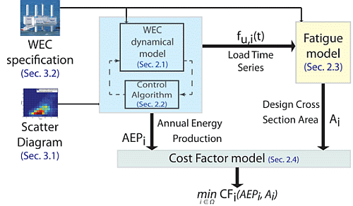

1. Introduction

Wave energy converters (WECs) have a high potential to contribute significantly to the world energy mix in the future. The practically exploitable wave power potential has been assessed to be up to 3.7 TW, which is about a fourth of the global demand and roughly a double of the global electrical consumption [1]. The global power consumption is ∼15 TW of which 10% is electrical power. A diverse spectrum of WEC prototypes has been realised, and further investigations on control strategies for electricity harvesting (see e.g., [2]) and structural design (see e.g., [3]) are ongoing.

In terms of maximum absorbed power namely reactive controller or maximum energy controller (MEC), the condition for optimality was firstly derived in the 1970s [4]. In recent years, the focus has moved to a more realistic implementation of the proposed controller, using both passive and active controllers. In the context of wave energy, the term “passive controller” refers to a purely resistive control strategy such as proportional (P) controller, latching control, etc. The implementation of this type of control has been proved to work both in numerical and physical models [5–10]. On the other hand, the term “active controller” refers to those control strategies that imply energy feedback to the converter in order to increase the overall absorption. This class includes proportional-integral (PI) controller [10], suboptimal (PIDc) controller [11,12], MEC [13] and others. Recently, the optimal control theory within the framework of model predictive control (MPC) has been introduced in order to incorporate constraints in the control problem [14–17]. The MPC groups both passive and active controllers together in function of the applied constraints as shown in [17]. The advantage of using MPC is that it overcomes both the unrealistic amplitude of motion predicted by the theory and the inability to handle constraints in theoretical formulations.

Overall, much effort has been put into finding the optimal control strategies where the main focus is the maximisation of the gained mechanical or electrical energy. Albeit maximising the absorbed energy is an important task, it has not been proven whether this is also optimal from an overall cost point of view. Since the global aim of the sector is the commercialisation of WECs, the economic quota needs to be considered too. For offshore structure, due to the high ratio between extreme and operational loads, the structural cost is expected to lie in the range 30%–50% of the capital cost [18,19]. This entails that the economic quota can be related to the structural dimension in the first approximation. When designing a WEC, besides the static load, the structure also needs to account for cyclic loads (fatigue) in the prospected lifetime. While the static loads are uncoupled to the chosen control algorithm, the fatigue behaviour of the WEC is coupled to the control strategy. Standards for oil and gas (see e.g., [20]) as well as offshore wind turbines [21–23] and (offshore) steel structures [24,25] recommend the use of Stress-Number (SN) curves for fatigue analyses of structural designs. The SN curve characterises the material performance concerning fatigue and shows the relation between the number of load cycles at a given stress amplitude leading to fatigue failure.

The work shown in [26] defines a first attempt to combine control and fatigue analysis, but only a simple passive control strategy is considered. In addition, neither constraints nor controller phase delay have been addressed.

The present article shows a simple non-recursive methodology to select the best control strategy for a given WEC where both energy absorption and structural design are considered. The methodology flowchart is presented in Figure 1. The dynamical model of the WEC is modified by a certain control strategy; five different strategies are used in the case study below. The WEC model receives the array of sea states as input, which defines the given location, and generates the annual energy production (AEP) for a given control strategy plus the time series of loads at the specific point selected for the fatigue assessment. The fatigue assessment is the second step of the algorithm, which receives as input the load time-series at a given location for a certain control strategy. Based on rain-flow counting [27] and offshore standards [22,24], the needed design cross section area for the given lifetime is evaluated. Derived from a simple parameterised, cost model the output from step one (AEP) and step two (material needed) can be combined. The control strategy leading to the lowest overall estimated cost could be chosen. The presented methodology is then applied to the Wavestar WEC [28] which is located at Danish Wave Energy Center (DanWEC) in Hanstholm (Denmark).

The paper is organised in five sections: Section 1 introduces the problem, together with the previous and proposed solution; Section 2 gives a general introduction of the different models used, namely WEC modelling, control problem and fatigue assessment; Section 3 specifies the equations presented in Section 2 for a particular WEC in a definite location; Section 4 contains a detailed discussion around the take-home messages embedded in the results; and Section 5 gives a brief recap of the work done besides the main outcome of the article.

2. Theoretical Background

A numerical model is used to describe the dynamical behaviour of a given WEC due to its flexibility. Despite the fact that numerical models are only an approximate representation of the corresponding physical models, once their accuracy is proven they represent a cheap and a fast tool for analysing a WEC, compared to physical modelling. In particular, numerical models based on linear potential theory coefficients require low computation cost whilst outputting accurate results if the motion of the WEC is kept bounded around the linearisation point [29,30].

It is important to bear in mind that the proposed numerical model is specified for WECs of the point absorber type due to the problem formulation simplicity, but the same approach can be used for a generic WEC of the activated body type after providing a representative model for the wave-body interaction. In the following, the definition of the used numerical model, control strategies and fatigue model composing the main algorithm are presented. The equations are expressed in the international system of units (SI) system of measurement and each parameter is expressed in accordance with the SI base.

2.1. Numerical Model

A WEC can be defined as a dynamic system with one or more degrees of freedom, used to transform the wave energy content into useful—typically electrical—energy. In this work, only the absorbed mechanical power will be considered. The transfer from mechanical to electrical power is not taken into account. A point absorber is a particular type of WEC where the characteristic length of the device is small compared with the wavelength. A single body floating system, like a point absorber WEC, presents a resonant-like behaviour similar to a mechanical oscillator. The dynamical model of system can be obtained using the Newton-Euler equation. If the system has only one degree of freedom, then the Newton-Euler equation is simplified to [13]:

$$\sum _i{F}_i=M\ddot{x}$$

(1)

where F_i represents a generic force/moment acting on the rigid body; M represents the mass/inertia of the body; and ẍ represents the body linear/angular acceleration. The wave-body interaction can be linearised around the equilibrium point by assuming small body motions (that is when the motion's amplitude is much smaller than the wave length) and by considering steady state conditions. According to the diffraction/radiation theory, the hydrodynamic problem can be dealt with as two subproblems. A third contribution in the force summation of Equation (1) comes in place from the linearised hydrostatic problem [13]:

$$F_{ex}+F_{\mathit{\text{RAD}}}+F_{hy}+\sum _i{F}_i=M\ddot{x}$$

(2)

where F_ex is the wave excitation force; F_RAD is the radiation force; and F_hy is the hydrostatic restoring force.

The wave excitation force is defined as an external force acting on the fixed structure subjected to a wave field and is defined by a complex function associated with the frequency of the incoming wave. It accounts for two distinct contributions namely the diffraction force plus the first order Froude-Krylov force evaluated for fixed wetted surface. The radiation force describes the loads acting on the structure due to its motion in still water and is defined as [13]:

$$\mathit{\text{FRAD}}(\omega )=V(\omega )[j\omega (A(\omega )-a_{\infty })+B(\omega )]=j\omega X(\omega )H_{\mathit{\text{RAD}}}(\omega )$$

(3)

where V (ω) is the Fourier transform of the velocity of the system; A(ω) is the added mass coefficient; a_∞ represents the limit value of the added mass when the frequency tends to infinity; B(ω) is the radiation damping coefficient; and H_RAD(ω) is the frequency response function of the radiation force per unit of body velocity. The hydrostatic restoring force, F_hy, describes the difference between gravitational force and the buoyancy force due to the submerged volume. F_hy is proportional to the body displacement, where the hydrostatic stiffness coefficient K_hy is the proportionality factor.

Equation (2) can be recast into Equation (4) by including the wave-body interaction [13]:

$$\left[j\omega (M+A(\omega )-a_{\infty })+B(\omega )+B_i+\frac{1}{j\omega }{K}_{hy}\right]V(\omega )=F_{ex}(\omega )+F_u(\omega )$$

(4)

where B_i represents any additional source of damping; and the summation of the external forces has been replaced by the control force (F_u). The control force represents the force imposed by the WEC's power take off (PTO) system, i.e., electrical generator. The effect of the controllable load into the body dynamic will be discussed in the next section. By taking the inverse Fourier transform, Equation (4) is mapped into the time-domain, leading to an integro-differential equation, commonly known as the Cummins equation [31]:

$$(M+a_{\infty })\ddot{x}(t)+{\int }_{-\infty }^t{h}_{\mathit{\text{RAD}}}(t-\tau )\dot{x}(\tau )d\tau +B_i\dot{x}(t)+K_{hy}x(t)=f_{ex}(t)+f_u(t)$$

(5)

where ẍ(t) is the body acceleration; ẋ(t) is the body velocity; x(t) is the body displacement; h_rad is the impulse response function of the radiation force; f_u(t) is the control force; and f_ex(t) is the wave excitation force. For a simple system such as a point absorber, the convolution integral can be efficiently substituted by a state-space model [32,33]. Even if the two formulations are both an approximation of the frequency response function, the state space model formulation is adopted when the model predictive controller is conceived, because the model of the WEC is built in a state-space form.

2.2. WEC Control Strategies

The average mechanical power (P̄) absorbed by a generic WEC over a time period (T) is the mean value of the product of the control load, f_u(t), and the body velocity in the used degree of freedom, ẋ(t) [13]:

$$\overline{P}=\frac{1}{T}{\int }_0^T{f}_u(t)\dot{x}(t)dt$$

(6)

The absorbed mean power is often used as a performance indicator for a generic WEC. The dynamic response of a WEC, and its production capabilities, is affected by the applied control scheme. Because the scope of the work is the balanced power optimisation of a WEC against structural fatigue, it is important to define both non-aggressive and aggressive controllers. In the context of this work, the term “aggressiveness of a controller” is meant in a qualitative sense. It refers to the actuator duty cycle.

Five different control strategies will be introduced and used in the case study. Three of them, P, PI and PIDc, are applied for the true comparison while the other two controllers (MEC and MPC) are employed as benchmarks. The P, PI and PIDc controllers have been chosen for their implementation simplicity and efficacy. They are listed in increasing aggressiveness order. The power performance of the three controllers will be compared with the maximum achievable mean power. The theoretical superior limit of P̄ depends on the model set-up; the simulation parameters are defined in Section 3.1. If the PTO is ideal, the MEC will define the WEC performance upper bound. On the other hand, if the PTO is not ideal, the MPC will be considered to be the optimal controller due to the inability of the MEC to handle physical constraints.

2.2.1. MEC

For a simple oscillator, the optimal energy transfer between external source and the moving body happens when the system is in resonance with the input's frequency. The analytical solution of the maximum absorbed power problem is [13]:

$$V(\omega )=\frac{F_{ex}(\omega )}{2(B(\omega )+B_i)}(7\text{a})$$

(7a)

$$F_u(\omega )=-Z_i^{*}(\omega )V(\omega )(7\text{b})$$

(7b)

where $Z_i^{*}(\omega )$ is the complex conjugate of the intrinsic mechanical impedance of the oscillator [13]:

$$Z_i(\omega )=j\omega (M+A(\omega )-a_{\infty })+B(\omega )+B_i+\frac{1}{j\omega }{K}_{hy}$$

(8)

Some considerations can be drawn from Equation (7):

• Since B(ω) is a real function, the resonance condition is achieved when the body velocity is in-phase with the wave excitation force (Equation (7a)).

• The power maximisation is an impedance matching problem [34]. Therefore, the control load needs to counteract the reactance of the oscillator (Equation (7b)).

• Some energy needs to be fed back to the floater during a wave cycle. Therefore, the actuator needs to be reversible, and the instantaneous power will be both positive and negative at different positions of the wave cycle.

• The actuator is considered ideal, i.e., there is no limitation on the force amplitude together with an unitary transfer function (no phase delay).

In addition to the inability to handle physical constraints and the unrealistic large amplitude of motion, the practical implementation of this type of controller is crippled by the non-causality of the control law. The definitions introduced in Equation (7) require information about the future incoming wave [13] and body velocity [35], which needs to be predicted. Given that the system is highly damped, the body velocity is a broad-band process, and its prediction cannot be reliable. On the other hand, under the assumption that the wave spectrum is a relative narrow-band process, its prediction can be considered reliable. Several works have addressed the issue of forecasting the incoming wave in the short range [36–38] for a real-time application of the controller. It is important to bear in mind that for a numerical simulation the input time series is known a priori, so there is no need to forecast the future waves since they are already available.

Among the two methods introduced in Equation (7), the reference velocity method (Equation (7a)) is adopted. In order to implement this type of controller, a low level velocity tracking system needs to be implemented; a PI controller has been chosen as a low-level logic.

Another issue arises when the reference velocity needs to be evaluated: the transfer function (TF) between the excitation force and the optimal reference is frequency dependent. This type of problem can be solved using an observer of the excitation force state, in the form of an Extended Kalman Filter [38] or a Hilbert Transform [39].

2.2.2. Model Predictive Controller

MPC refers to an advanced, digital control technique. Its basic principle is to calculate optimal values for the control signals over a certain time horizon in the future. To this end, it uses a dynamic model of the plant, current measurements to update the dynamic states of this model, and the future course of external inputs; the latter being the wave excitation force and the control force in this paper. Given that the dynamic model sufficiently represents the real system and that measurements for updating the states and a prediction of the future wave excitation force are available, the WEC's behaviour over the time horizon can be calculated depending on the control force. This is used to determine the optimal trajectory of the control force by solving a possibly constrained optimisation problem. This optimisation problem includes a cost function that reflects the control objectives. The optimal control force is then applied to the point absorber until the new measurement and predictions samples are available. After that, the whole procedure is repeated in order to account for unforeseen disturbances. The ability of directly incorporating constraints in the optimisation problem makes MPC a straightforward choice for control problems with constraints on the control input or the plant states.

Several applications of MPC for the control of WEC are reported in the literature. Some of them directly incorporate the objective of maximum average power into the cost function [14–17]. For this work, the variant presented in [17] was chosen. It uses a non-standard method for deriving the time discrete model from the time continuous model in Equation (5). The resulting control algorithm allows for relatively large sample periods without degrading the accuracy. Large sample periods are generally desirable because the computational effort in solving the optimisation problem at every time step is large.

The general formulation of the applied cost function J is the time discrete version of Equation (6), that is [17]:

$$J[k]=\sum _{i=k}^{k+N_p}{f}_u[i]\dot{x}[i]$$

(9)

where k ∈ ℤ denotes the current time instant; and N_p is the number of time steps of the prediction horizon. The overall optimisation problem with the constraint on the control force can be written as [17]:

$$\begin{array}{cccc}\underset{f_u[i]}{\mathit{\text{maxJ}}}[k]& \text{such that}& |f_u[i]|\le f_{\mathit{\text{max}}},& i=k,\dots k+N_p\end{array}$$

(10)

If feasible, the solution of this problem yields an optimal control sequence over the prediction horizon. Using the receding horizon control principle, only the current sample f_u[k] is applied to the WEC, leading to the ability of the controller to react to unforeseen disturbances. The whole problem formulation can be found in [17]. Here, it should only be noted that for using computationally efficient algorithms to solve Equation (10), the defined optimisation problem has to be convex. Reference [17] shows that the cost function (Equation (9)) leads to a quadratic program, i.e., linearly constrained optimisation problem with a quadratic objective function. Although no universal proof of its convexity is given, this property can be ensured by a numerical check after the design of the controller.

2.2.3. P Controller—Passive Controller

When the WEC actuator only works in an unidirectional mode, no energy can be fed back to the oscillator. This type of controller commonly known as passive damper has the great advantage of requiring simple machinery and having a smaller ratio between peak average power. Otherwise, since the body reactance will not be compensated, the WEC will mainly work in a tight range around the natural frequency of the oscillator, limiting the overall system efficiency. The general form of the control force is as follows [10]:

$$f_u(t)=c_c\dot{x}(t)$$

(11)

where c_c is the damping coefficient of the control force.

2.2.4. PI Controller—Spring-Damper Controller

The PI controller is also denoted as spring-damper controller because an additional term proportional to the body displacement is used to compensate the intrinsic reactance of the body. In theory, the PD controller can also achieve similar results, but as shown in [10] it presents a narrower frequency band, which leads to a lower overall efficiency. These type of controllers are optimal controllers in the case of regular waves, but they become non-optimal for irregular waves. The downgrade is related to the lack of compensation of the memory term of the fluid. In fact, the optimal control law needs to include the convolution term related to the fluid memory, as can be derived from the application of the Pontryagin's maximum principle [12]. The general form of the PI control force is as follows [10]:

$$f_u(t)=c_c\dot{x}(t)+k_{c}x(t)$$

(12)

where k_c is the stiffness coefficient of the control force.

2.2.5. PID Controller with Memory Compensation—Sub-Optimal Controller

The PID controller is a mass-spring-damper controller with the introduction of an additional convolution term. The general form of the controller is as follows [12]:

$$f_u(t)=c_c\dot{x}(t)+k_{c}x(t)+m_c\dot{x}(t)+{\int }_{-\infty }^t{h}_{\mathit{\text{RAD}}}(t-\tau )\dot{x}(\tau )d\tau$$

(13)

where m_c is the mass coefficient of the control force. The convolution integral of Equation (13) represents the compensation of the memory term of the fluid (i.e., radiation force). This type of controller is a sub-optimal controller because it approximates the optimal non-causal solution with a causal one [12,35]. In order to avoid the uncertainties related to the body velocity prediction, see Section 2.2.1., the integral term concerning the time interval from t + δt to ∞ is neglected.

2.3. Fatigue Assessments

Fatigue failure is an important failure mode of offshore structures and expectably even more for WECs where the resonance condition is sought. For estimating the fatigue of a structural part, the Stress-Number (SN) of cycles curve together with Miner's rule [40] is used here. SN curves for offshore applications can be found in [24]. Miner's rule uses sequence independent linearised damage accumulation and assumes that fatigue failure occurs when [40]:

$$\sum _{i=1}^{N_i}\frac{n_i}{N_i}=1$$

(14)

where N_i is the total number of cycles of a given stress range leading to fatigue failure; and n_i the expected number of cycles at the same stress range during the life-time of the WEC. The SN curve shows the number of cycles leading to fatigue failure of a given stress amplitude. When using the SN approach, a linear or bilinear formulation, where plastic deformation is allowed, can be implemented. Rain-flow counting (see [27]) can be used to discretise the load time series into groups/intervals of load amplitudes. A certain interval i has n_i cycles per year of a certain load range ΔQ_i (e.g., normal force). It is assumed that the stress range Δσ_i can be expressed by a design parameter z (e.g., cross section area) and the corresponding load range ΔQ_i:

$$\mathrm{\Delta }{\sigma }_i=\frac{\mathrm{\Delta }{Q}_i}{z}$$

(15)

The bilinear SN curve has a slope change at Δσ_D where the number of cycles to failure N_D is equal to 1 × 10⁶:

$$\begin{array}{lll}N=K_1{S}^{-m_1}\hfill & \text{for}\hfill & S\ge \mathrm{\Delta }{\sigma }_D\hfill \\ N=K_2{S}^{-m_2}\hfill & \text{for}\hfill & S<\mathrm{\Delta }{\sigma }_D\hfill \end{array}$$

(16)

where K_1,2 are the stress intensity factors; and m_1,2 are the crack growth parameters. A design equation can be used to calculate the design equation parameter z and can be written for a bilinear approach using the Miner's rule as, see e.g., [41]:

$$1-\underset{S\ge \mathrm{\Delta }{\sigma }_D}{\underbrace{\sum _i\sum _j\sum _{k_1}\frac{T_{\mathit{\text{FAT}}}{n}_{ij{k}_1}}{K_1^c}{s}_{ij{k}_1}^{m_1}P(H_{m{0}_i},T_{Pj})}}-\underset{S<\mathrm{\Delta }{\sigma }_D}{\underbrace{\sum _i\sum _j\sum _{k_2}\frac{T_{\mathit{\text{FAT}}}{n}_{ij{k}_2}}{K_2^c}{s}_{ij{k}_2}^{m_2}P(H_{m{0}_i},T_{Pj})}}=0$$

(17)

where log(K^c) is the characteristic value of log (K); n_ijk is the number of stress ranges per year given the significant wave height H_m0i and the wave peak period T_Pj; s_ijk = ΔQ_ijk/z is the stress range ijk given H_m0i and T_Pj. The fatigue design life T_fat is equal to FDF · T_L with fatigue design factor (FDF) and design life time T_L. The joint probability of H_m0i and T_Pj is equal to P(H_m0i,T_Pj) = P(H_m0i)P(T_Pj|H_m0i) and indicates the probability of occurrence of a certain sea state.

2.4. Cost Factor

This section focuses on bringing together the influence of a certain control strategy on harvested energy, which will define the income during lifetime, and the resulting structural design which drives the investment costs. In order to compare different control strategies, a simple economical model is used.

From a certain structural detail, one can hardly comment on the control strategy's overall cost impact. But one can, based on some simple assumptions get an idea of the relative impact of the different control strategies on the overall cost.

It is assumed that the total lifetime costs consists of one part, which is dependent on the control strategy (called C₁, mainly cost for PTO and structure of PTO arm) and other investment costs (called C₂, e.g., platform, or electricity connection to shore), which are assumed to be constant for all control strategies. The control dependent costs are assumed to be proportional to the cross sectional area of a certain critical structural component. The cost factor CF_c, which shows the ratio between total investment costs and the absorbed energy (AEP_c), for a given control strategy c can be written as:

$$C{F}_c=\frac{C_1+C_2}{E_c}=\frac{p\cdot C_{\mathit{\text{ref}},\mathit{\text{tot}}}\frac{A_c}{A_{\mathit{\text{ref}}}}+(1-p)\cdot C_{\mathit{\text{ref}},\mathit{\text{tot}}}}{AE{P}_c}$$

(18)

where C_ref,_tot is the total lifetime cost of a certain design with a reference control strategy; A_ref is the cross sectional area of a critical structural component for the reference control strategy; A_c is the resulting cross sectional area of control strategy c; and p represents the percentage of the total lifetime costs, which are dependent on the control strategy. Even though the main assumption adopted—linear relation between WECs cost and structural dimensions—is rather stringent, the cost factor can still give a valuable tool to gain insight into the economic potential of a WEC and afterwards ease the comparison between proposed concepts.

3. Case Study Results

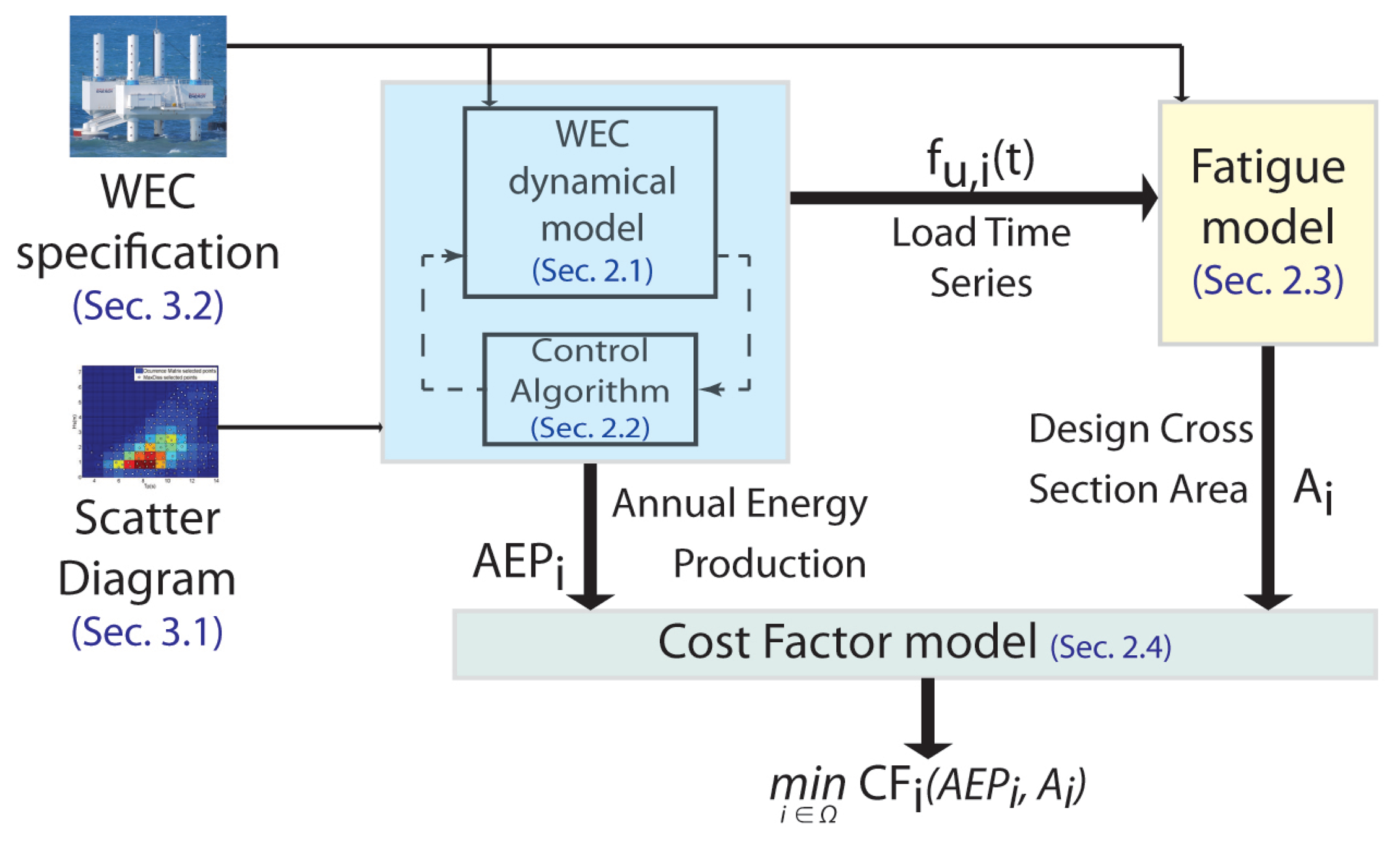
This section presents a case study focused on the Wavestar WEC. The particular WEC has been chosen mainly because its numerical model already has been compared with experimental data from a scaled physical model of the device [29,30]. The effect of different control strategies and constraints on the power output as well as the fatigue of different subcomponents are assessed. The Wavestar device is located at DanWEC (Danish North Sea coast) near Hanstholm. This prototype (see Figure 2) consists of four piles and two floaters as well as a platform where the mechanical and electrical devices are stored. The floaters which are excited by the passing waves drive a hydraulic system which impels a turbine and a generator. The Wavestar device was installed in 2009 and fed electricity into the grid until it was moved to the harbour for reconfiguration in September 2013.

3.1. Site Assessement

Sea state measurements over a period of six years are provided by [42], based on recordings from a buoy (6332100N, 474700E, water depth: 17 m) located near the Wavestar device. The dataset contains the frequency domain wave parameters, significant wave height (H_m0) as well as the peak period (T_P), measured with a time interval of 3 h. The resulting probability of occurrence of different wave states are shown in

Table 1. Relative occurrence of different wave states from six years, buoy measurements ([H_m0] = m, [T_P] = s). Both parameters defines the mean value over an interval. The adopted discretisation is 1 s in T_p and 0.5 m in H_m0.

Hm0/TP	0.5	1.5	2.5	3.5	4.5	5.5	6.5	7.5
0.25	-	-	-	0.04	0.04	0.02	0.01	-
0.75	-	-	-	0.07	0.17	0.11	0.05	0.01
1.25	-	-	-	-	0.06	0.11	0.05	0.01
1.75	-	-	-	-	-	0.06	0.05	0.02
2.25	-	-	-	-	-	0.01	0.05	0.02
2.75	-	-	-	-	-	-	0.01	0.02
3.25	-	-	-	-	-	-	-	0.01

and are used in this case study.

The incoming wave direction is not considered in this case study and is assumed to be of minor importance for the load and power output assessment, as a consequence of the symmetry of the system.

3.2. Numerical Model of the Wavestar WEC

Since the Wavestar machine belongs to the point absorber WEC class, the model introduced in Equation (5) can be used to describe the dynamic response of the system.

Table 2. Model parameters for the Wavestar WEC [10,30,45]. TF: transfer function.

Hydrostatic and structural parameters
Moment of Inertia	Jst	2.45 × 106	kg·m2
Hydrostatic Stiffness	Khy	14.0 × 106	N·m/rad
Maximum exerted moment	Mmax	1.0 × 106	N·m
Drag Coefficient	CD	0.25	-
PTO stroke	Spto	2.0	m
Natural Period in Pitch	Tn	∼3.5	s
Hydrodynamic model parameters
Added mass at infinity frequency	a∞	1.32 × 106	kg·m2
Radiation Moment TF numerator	aRAD	[4.93, 1.08] × 106	-
Radiation Moment TF denominator	bRAD	[1, 2.56, 5.16]	-
Excitation Moment TF numerator	aEX	[5.4 × 1010, 2.7 × 1012]	-
Excitation Moment TF denominator	bEX	[3.6 × 104, 3.9 × 105, 1.5 × 106 2.6 × 106, 1.6 × 106]	-

and Figure 3 summarise the model parameters used in this case study.

For each sea state described in Table 1, a surface elevation time series of 30 h is fed into the numerical model. The time series' length is determined by the need to minimise the statistical uncertainty of the model input, related to the irregularity of the wave. The White Noise filtering technique is adopted to generate the surface elevation time series, using Wavelab [43]. The filter uses a JONSWAP spectral model [44] with peak enhancement factor (γ) equal to 3.3 and a sample frequency equal to 20 Hz.

The linear hydrodynamic coefficients as well as the hydrostatic stiffness coefficients have been evaluated using a commercial Boundary Element Method (BEM) solver [45]. The radiation frequency functions plotted in Figure 3 have been interpolated with a rational polynomial approximation, whose order is reduced using the Hankel singular value [32]. The resultant second order TF is listed in Table 2. Order reduction is an important topic mostly in the MPC formulation because of computational time, but for consistency the minimum order model has been adopted throughout the work.

The power performance of the WEC is evaluated for the unconstrained model and for two other cases, all defined in Equation (5):

• Case 1—Unconstrained case. Neither the saturation of the maximum PTO force, nor the maximum allowed PTO stroke, nor the additional damping is included.

• Case 2—Unconstrained case with linearised viscous drag moment implemented as additional damping. Neither the saturation of the maximum PTO force, nor the maximum allowed PTO stroke is included.

• Case 3—PTO constraint and linearised viscous drag moment implemented as additional damping. The PTO constraint is implemented as a saturation function of the full control force.

Hereafter, the rationale behind these choices is briefly given. The linearised viscous drag moment has been inserted in the WEC model in order to account for a viscous dissipative effect. This type of effect is normally negligible when the system operates in a non-resonant condition due to the relative low body velocity. On the other hand, when the resonance condition is achieved, a significant part of the energy is dissipated in turbulence [46]. Given that the main focus of the work is on the implementation of optimal control strategies, the viscous drag moment is likely to play an important role in the assessment of the absorbed power. The viscous drag coefficient reported in Table 2 has been obtained from laboratory tests [30].

The PTO constraint is introduced to simulate a model as close as possible to the device deployed at DanWEC in Hanstholm (Denmark). This type of constraint reflects a realistic feature of many types of actuators, to be used in a WEC, and it is worth investigating its effect in both power and fatigue assessment. The PTO constraint is taken from [10]. All the parameters presented are summarised in Table 2. The simulations were carried out using the Simulink/Matlab environment.

In order to simulate a realistic PTO system, two other parameters were identified besides the saturation function applied in Case 3:

• Case 4—End-Stop of the PTO actuator. Another external force is added in the force summation in the right hand side of Equation (5). The force is proportional to both the penetration of the piston into the end-stop system and the penetration velocity.

• Case 5—PTO delay [10]. In this case, a second order TF is applied to the theoretical control force $f_u^i(t)$ in order to obtain the true control force f_u(t).

In both cases, the PTO was saturated as in Case 3. The sensitivity analysis of the WEC model response with respect to these two additional cases shows that the PTO constraint is the most critical parameter. In fact, in Case 4, the End-Stop system is rarely exerted as a result of the non-optimality of the controller induced by the limited PTO capacity. Further, in Case 5, the PTO delay is small compared with the system dynamic. Therefore, the induced phase shift accounts for only a small reduction of the power performances. Since the contribution of Cases 4 and 5 is below 1% in both AEP and cross section area, these cases will be omitted in the following.

3.3. Control Strategies of the Wavestar Device

The controller schemes presented in Section 2.2 have been introduced into the WEC model in order to estimate its average power performances. As shown in Figure 1, the implementation of the dynamical response of the WEC is uncoupled with the structural fatigue assessment:

• P—proportional or passive controller (Section 2.2.3.);

• PI—proportional-integral or spring-damper controller (Section 2.2.4.);

• PIDc—proportional-integral-derivative with memory compensation or sub-optimal controller (Section 2.2.5.);

• MEC—maximum energy controller (Section 2.2.1.);

• MPC—model predictive controller (Section 2.2.2.).

The MEC is considered a benchmark for Cases 1 and 2 since it defines the theoretical upper bound of the absorbed energy. For Case 3, the MPC will be considered as reference point; the MEC is indeed unable to deal with constraints. The remaining controllers are then used to assess the effect of control aggressiveness into the absorbed power.

The MPC cannot be considered an applicable controller in the present formulation, because in the simulations the control algorithm was assumed to have perfect knowledge of the future excitation moment over the full prediction horizon. Therefore, uncertainties related to the excitation moment prediction are discarded with a reasonable increment of the power performance. Furthermore, the current state of the plant is assumed to be perfectly known. Hence, the MPC results are considered an upper bound in terms of the objective function rather than a practicable solution in the present formulation. The implementation of the different controllers is described in detail in the following.

The MEC is implemented using the velocity tracking logic where the velocity signal is generated in two steps: first, the actual wave frequency and amplitude are observed using the Hilbert transform [39] and, second, the observed frequency and amplitude are used in a look-up table to recover the reference velocity at the actual sample time. The general control layout traces out the implementation presented in [47]. The Ziegler-Nichols closed-loop tuning method was used to tune the PI low-level velocity controller [48].

The MPC model is based on the state-space approximation of the WEC model summarised in Table 2. The sample time employed in the MPC is 0.05 s. The other important parameter used to tune the performances of the MPC is the length of the prediction horizon, N_p. At each time sample, the optimiser searches the optimal trajectory over the prediction horizon using the Hildreth's quadratic programming algorithm [49]. The computational cost of this method is a cubic function in the N_p variable. Recalling that the simulation time length is 30 h, it is clear how the definition of N_p becomes a crucial point. The best compromise between MPC performance and computational time was found to be N_p = 120, with negligible degradation of the power performances if compared to the MEC in the unconstrained case. Using this set of parameters, the MPC roughly foresees one full wave ahead. The MPC predicts the same AEP of the maximum energy controller in Cases 1 and 2, as will be presented in Figure 4. The difference between the two controllers grows as the wave period increases, because the prediction horizon becomes too short. In the considered case study, the probability of occurrence of the long period sea state is relative low, which reduces the global influence of the actual MPC set up error. Depending on the specific scatter diagram, N_p needs to be adapted to the current sea state. The adjustment will be based on the results of a sensitive analysis on the power performance of the WEC in function of N_p.

Controllers P, PI and PIDc have already been defined up to the establishment of the control parameters (c_c, k_c, m_c). They have been assessed using a global maximisation routine, whose objective function is the mean absorbed power. The global maximum point is obtained using a local maximisation algorithm (Nelder-Mead method [50]) with randomly seeded starting points (scattered search [51]). The algorithm is repeated for each sea state, each controller and each case.

A special attention needs to be given to the PI and PIDc controllers when the PTO moment is constrained. In order to reduce the error accumulated in the integrator introduced by the abrupt saturation, an integral windup with back-calculation scheme was used [52]. The main improvement given by the windup scheme is a reduction of controller overshooting.

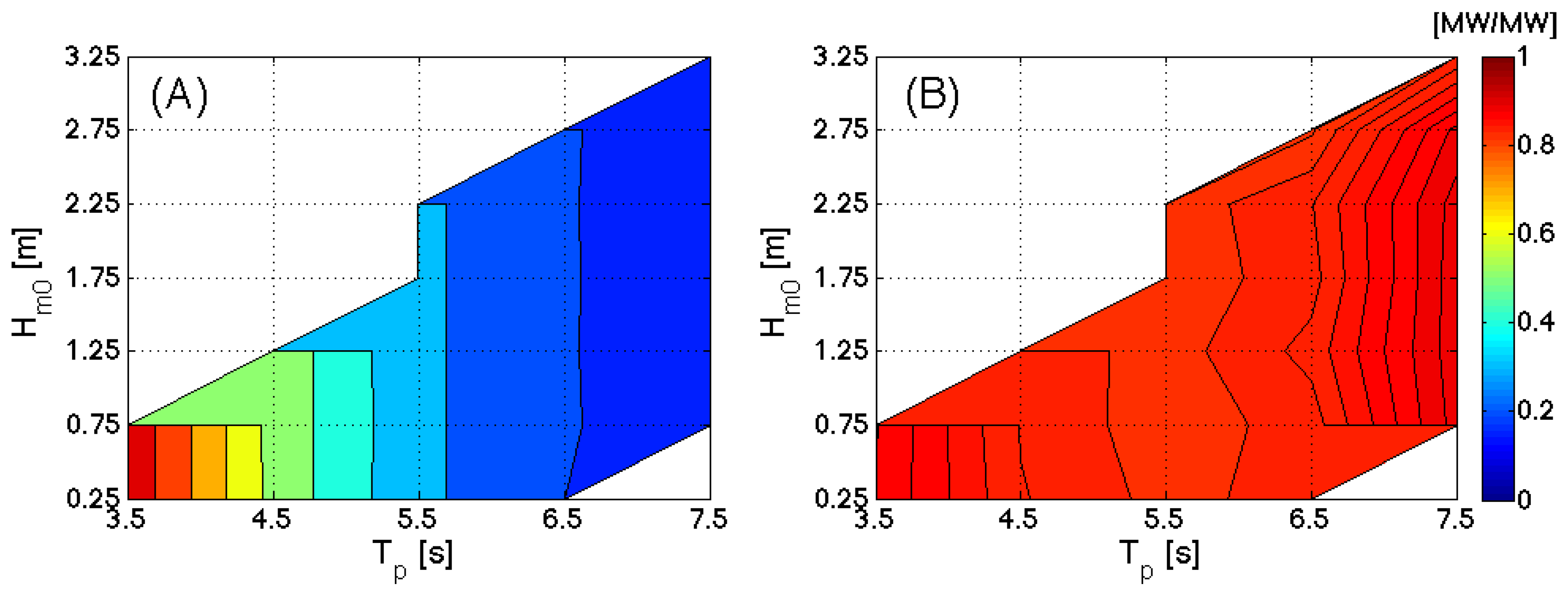
The absolute performance of the different controllers is quantified using the power matrix, which defines the average power production for each simulated sea-state. Figures 5 and 6 report the power matrix of P and PI controller, for the unconstrained (Case 1) and PTO constrained cases (Case 3), normalised by the benchmark controller power matrix. As introduced in Section 2.2.3., the passive control strategy is unable to tune the response of the oscillator to the incoming wave frequency. Therefore, only sea-states with T_p close to the natural period T_n of the system will have a power production equal to the reference point. The performances of the P controller reduce quickly as T_p moves away from T_n (Figure 5A); the natural period of the floater is ∼3.5 s. On the other hand, since the PI controller can extend the bandwidth of the oscillator, it will result in a power performance similar to the benchmarks (MEC), which is shown in Figure 5B.

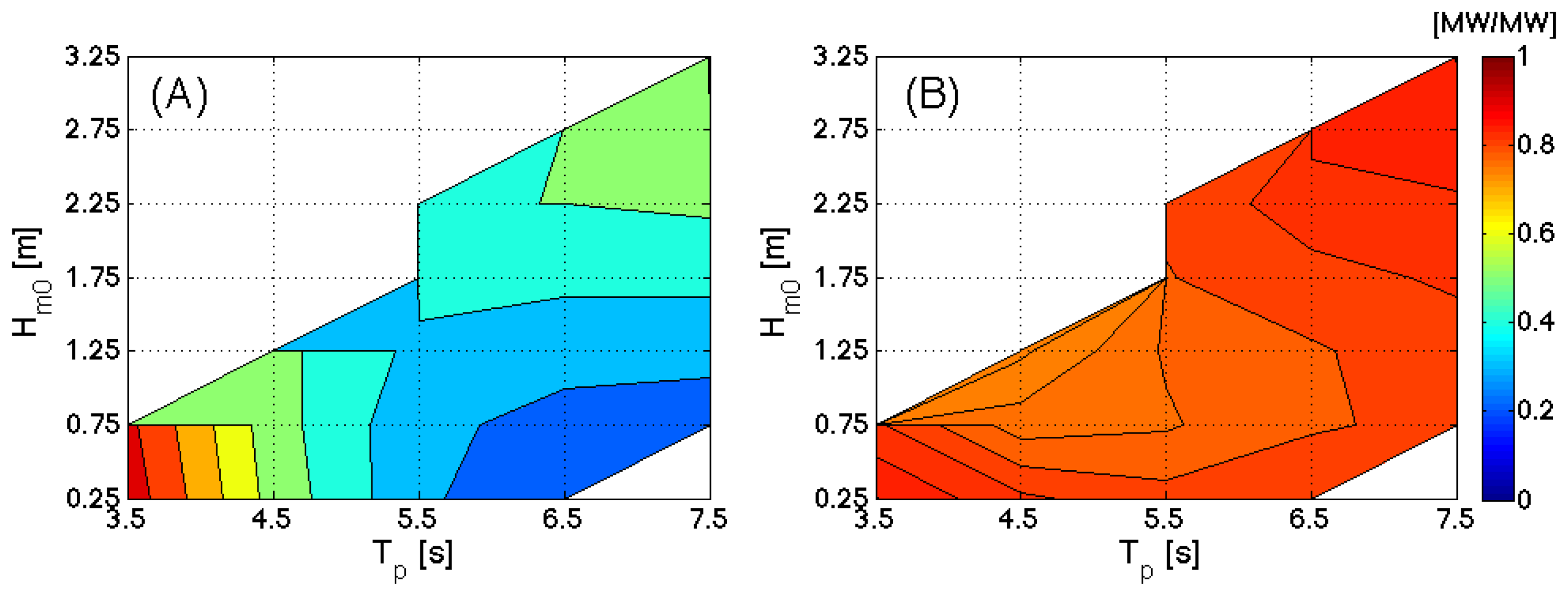
Moreover, when the PTO moment is bounded, most of the energy in the high energetic sea-states cannot be absorbed (Figure 6A), leading to a better relative performance of the P controller relative to both the benchmark (MPC) and PI controller. As introduced in Section 2.2, the benchmark changes as the considered case changes. It is important to notice that the power performance of the MPC worsens when the PTO saturation is included, while the P controller does not undergo significant performances variations. This fact is in connection to the relatively smaller control moments commanded by the P controller, relative to the other controllers. Figure 6B shows that the PI controller can handle PTO constraints almost without losing performance when compared with the MPC. A direct consequence of this lies in the practical applicability of the controller. Taking into account the implementation simplicity of the PI controller and its negligible power performance reduction in the constraint case, this method becomes much more attractive than the MPC, provided an effective sea state adaptation of the PI controller parameters is available.

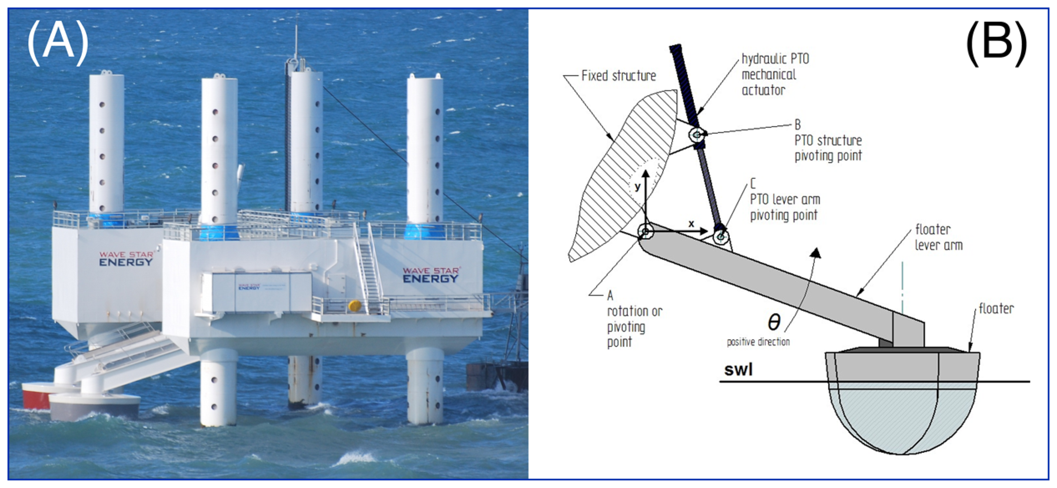
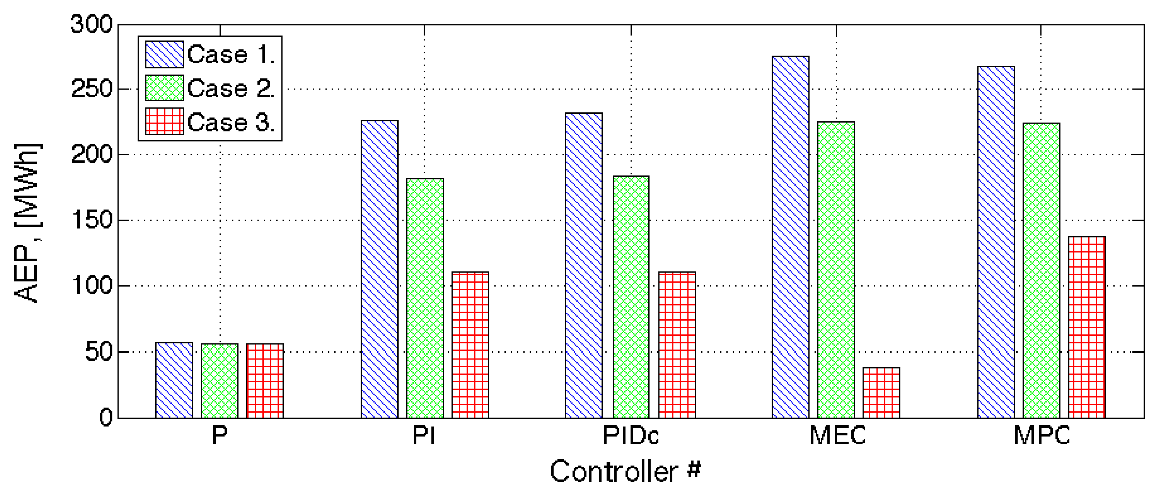
Using the power results of the Wavestar WEC and the scatter diagram shown in Table 1, the AEP can be evaluated. Unlike the power matrix, the AEP should be regarded as the global relative energy performance indicator of the particular WEC at the specific location. In Figure 4, the AEP of the Wavestar WEC at the Hanstholm location is given for each case and controller.

The energy performance of the P controller can be increased reasonably by a factor of two when an active controller is adopted into the WEC model. The five-fold increase of the unconstrained case is mainly linked to the unrealistic motion amplitude achieved in the high-energetic sea states. In those conditions, the linear theory assumptions are heavily violated, and the simulation results become unreliable. The viscous dissipative term accounts for a global performance reduction of up to 15% if an active controller is used. For the passive controller, the small body velocity induced by the non-resonant WEC makes the turbulence effect negligible [30].

Both active controllers used (PI and PIDc) show similar results. In addition, their operation is close to the benchmark capability. Given that the performance gap does not seem to be a function of the applied constraint, it is reasonable to assume that both PI and PIDc controllers have a flat power performance compared with the optimal controller. This trend is also visualised in Figures 5 and 6B.

3.4. Fatigue Assessment

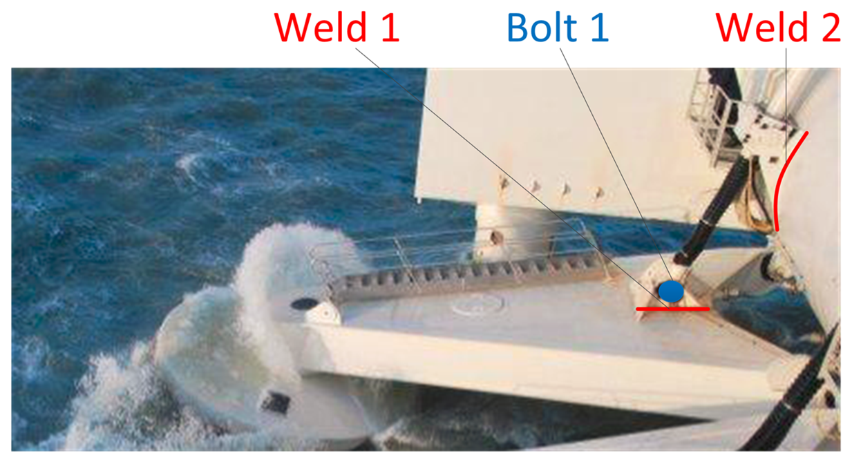
For the fatigue assessment, the focus is put on different components of the floater arm. Due to the fact that the floater can be taken out of the water during storm events, extreme events are of minor importance for the structural design of the floaters. Critical subcomponents whose failure may lead to an overall breakdown are bolted as well as welded connections. Therefore, the focus here is on the two welded details and one bolted connection shown in Figure 7. Failure of one of these would lead to structural failure of the arm due to inability of controlling the motion of the arm. Time-series of loads of 30 h are compiled for different control strategies and each wave state shown in Table 1.

Table 3. Parameters of Stress-Number (SN) curves shown in Figure 8 for the three different considered connections at the Wavestar WEC. The parameters are taken from [24].

	m1 (-)	log(K1) (-)	m2 (-)	log(K2) (-)
Weld 1	3	11.455	5	15.091
Weld 2	3	11.455	5	15.091
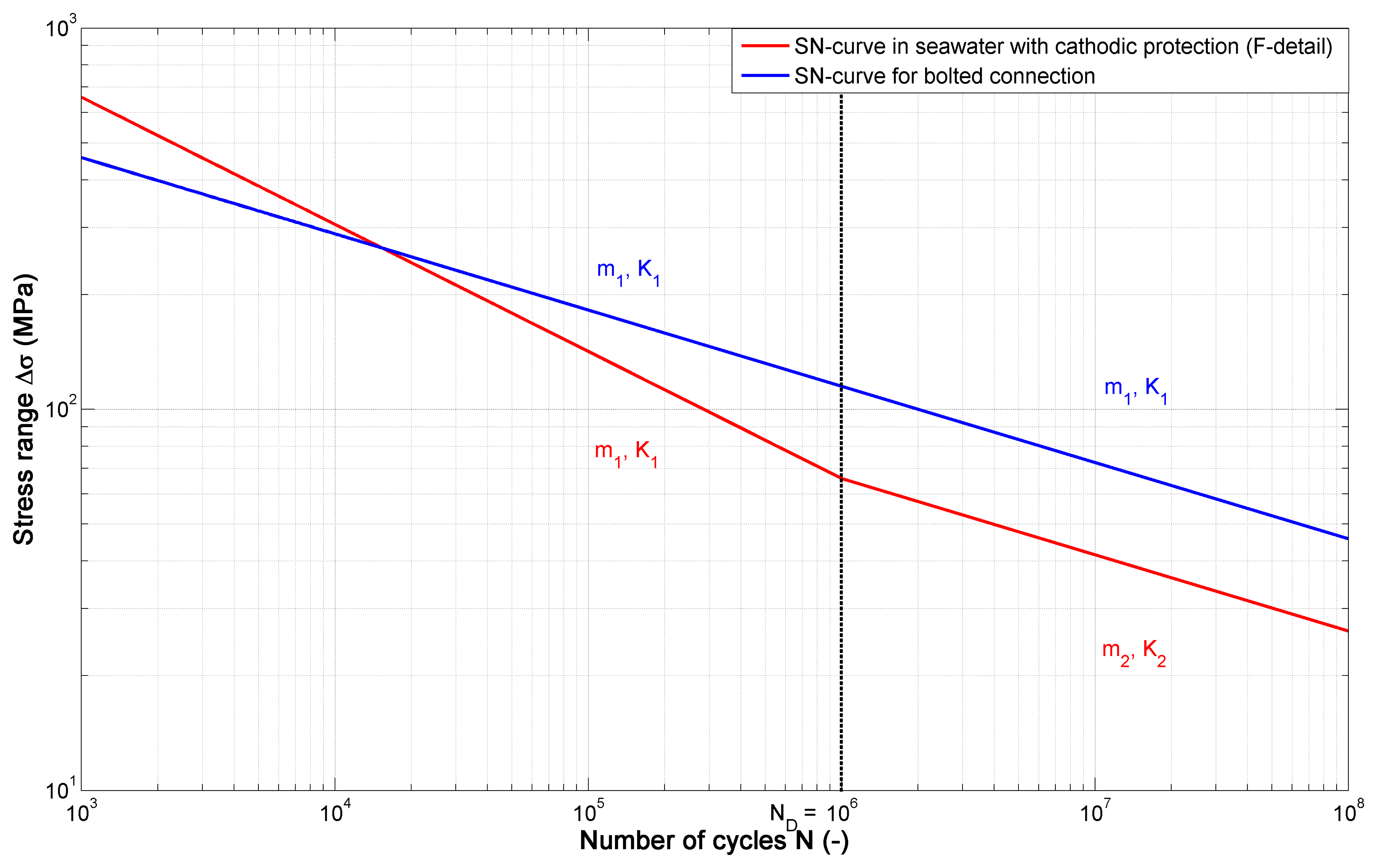
Bolt 1	5	16.301	-	-

and Figure 8 show the two SN curves, taken from [24], used in this case study. Weld 1 is located at at a cruciform joint, and Weld 2 is placed parallel to the direction of applied stress. Fatigue behaviour of both welds can be explained considering the SN curve of a so-called “F” detail [24]. Here it is assumed that cathodic protection is used. The bolted connection between the arm and the PTO is in double shear. According to [24] for bolts in shear a linear SN curve should be done. The SN curve is defined by the parameters m₁ and m₂, which are equal to the negative inverse slope of the SN curves and log(K₁) as well as log(K₂), which show the intercept of log(N) axis.

The life time T_L of the Wavestar power plant is assumed to be 20 years, and no maintenance actions are considered here. The fatigue design is performed with a FDF of 3, which is in accordance with [22] for details which are not inspected.

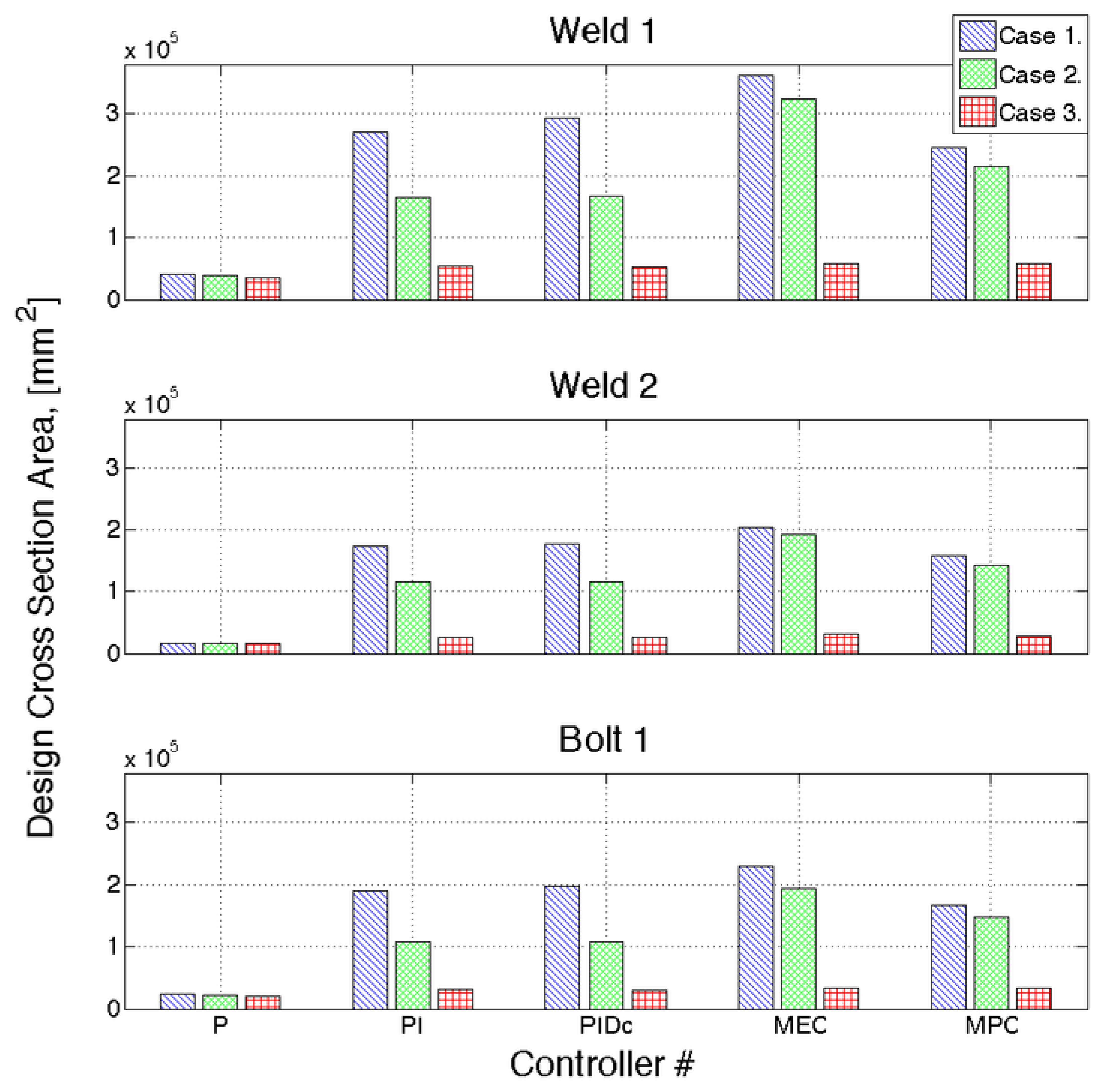
Figure 9 shows the design cross section area of the three different connections defined in Figure 7 for different control strategies as well as different cases. The design cross section area is meant to be the cross section area resulting from the design. In general, different control strategies as well as different cases lead to different cross section areas. The simplest control strategy leads to the smallest fatigue loads onto the structure and, therefore, to the smallest cross section area. For this control strategy, the impact of different cases is negligible. For all other controllers, the unconstraint case (Case 1) gives the largest cross section areas. When viscous drag effects on the floater are included (Case 2), the loads onto the structure are decreased compared with Case 1 and, therefore, the needed cross section is reduced. The smallest cross section areas are reached in Case 3 where the PTO maximum deliverable moment is included in the simulations.

Figure 10 shows the number of expected cycles during 20 years for Weld 1 using MPC with different cases. Figure 10A shows the expected number of cycles, n₁,_i, during one life-time of 20 years for a given load range ΔQ_i in the unconstraint Case 1 whereas Figure 10B shows the number of expected cycles, n₂,_i, for MPC given constraint Case 3. Part C in Figure 10 shows the difference between the number of expected cycles during one life-time for a given load range. The constraint leads to more cycles with small and load amplitudes equal to the constraint whereas the unconstraint case leads to a small number of loads with large amplitude. Cycles with large load amplitudes have a large impact on fatigue due to the fact that the number of cycles up to failure for a given load range relates exponentially to the load range (see Equation (16)). This small number of large loads are the reason why the design cross section area is increased for Case 1 (unconstraint) by a factor of 5 (see Figure 9) compared with Case 3 (constraint).

4. Discussion

In the following, the discussion of the results for the specific case study elaborated in Section 3 is given. It is important to bear in mind that whilst the proposed method can be extended, prior to modification, to other WECs of the activated body type, any extrapolation of the results of Section 3, for any other device, should be considered inaccurate. Different conclusion should also be expected if different connection points are chosen for a given WEC.

Figure 11 shows the comparison between the AEP and the cross section area of Weld 1 for Case 1 (A-Unconstrained case) and Case 3 (B-PTO constrained case) in function of the applied control strategy. The data is normalised by the results of Case 1, MEC. The PTO constraint induces a two-fold reduction of the AEP of the WEC, but it also drives a similar mitigation of the structural fatigue of Weld 1. The same conclusion can be drawn for the other connections. The usage of the PI controller leads to a two-fold growth of the AEP of the WEC, keeping the increment of the required cross section area to 1.5-fold. The AEP defined so far is related to the absorbed energy. If a PTO efficiency of 70% between the absorbed energy and the electrical energy produced is adopted, the AEP will vary. The AEP of the P controller will be reduced by 30% while the AEP of the PI controller will suffer a larger reduction, due to the doubling of losses exerted in the bidirectional process, [53]. In addition, when an active controller is used, the system complexity will increase with respect to a simple passive controller, which might induce a reduction in availability of the WEC.

Based on the cost factor, CF (see Equation (18)), different control systems can be compared on an economical level. It is assumed that the critical structural component, whose cross section area is used for calculating the cost factor, is Weld 1. Figure 12 shows CF values, which are normalised by the CF value of Case 1 and p = 0%, for different control strategies. As expected, the normalised CF increases when p is increased. The impact on the p-value is larger for Case 1 but for Case 3, the p-value impact is of minor importance. For Case 3, the different CF values are mainly driven by the different control strategies and its resulting AEP. Lowest CF values are for all p values reached when using the MPC controller.

A sensitivity analysis has been carried out in order to investigate the impact of detuned control parameters on AEP and cross section area.

Table 4. Results of the sensitivity analysis for P and PI controller. Variation of the cross section area (red text) of Weld 1 and annual energy product (blue text), normalised by the controller where AEP is maximised.

	P controller	PI controller
		1.2 kc	kc	0.8 kc
1.2cc	+5%	+1%	−3%	−10%
	−1%	−3%	−3%	−8%
cc	0%	+4%	0%	−8%
	0%	−2%	0%	−5%
0.8 cc	−6%	−5%	+3%	−5%
	−1%	−5%	−1%	−4%

shows the AEP and cross section area of Weld 1 for P and PI controller, using Case 3 (constraint plus viscous drag). The P and PI power optimised gains are detuned by ±20% and the results are normalised by the AEP maximised case; c_c is the proportional gain and k_c is the integral gain.

As expected, the AEP is reduced in all cases, while the fatigue loads acting on the structure can be reduced by choosing the right detuning combination. From an economic point of view, only those cases where the reduction of power output comes along with reduced fatigue loads are of potential interest.

This is clear in the case of the P controller where the amount of damping is positively correlated to the structural load, and only the reduced damping coefficient (0.8c_c) can be considered. Figure 13 shows the variations of CF with respect to the p-parameter obtained from Equation (18). When the cost is assumed to be independent from the control strategy, i.e., p = 0%, then CF is greater than one. There is a break-even point at p* = 16.7%. That is, if the part of the cost that is influenced by the controller makes more than 16.7% of the overall costs, then it is economically wise to apply the detuned coefficient.

For the PI controller, Figure 14 shows the variation of the cost factor for all the cases from Table 4 and for p = 10%. The contour plot indicates that for p = 10% the power-optimal controller is also economically optimal. The best detuned controller happens at 100% c_c and 80% k_c, but in this case the break-even point is p* = 68%. Up to now, only very little cost data is publicly available for WEC (see e.g., [54]). Hence, for a rough estimate of an upper bound of p, it is possible to look at the figures in the offshore wind sector. The capital expenditure varies between 50%–70% of the overall life-cycle costs of an offshore wind turbine [54–57]. The costs of the turbine itself make about one third of it [58,59]. That is, the value of p is very likely to lie well below 0.7 × 0.33 (23%). Transferring this p-value to the WECs, shows that only for the P controller economic improvement is realistic by detuning controller parameters. The higher break-even point of the PI controller compared to the wind turbine case leads to the conclusion that detuning the parameters does not seem to be a reasonable choice. Albeit the above parallel give some indication whether the CF is affected by the detuned control gains, it is important to bear in mind that due to the variety of WEC concepts the comparison is somehow coarse.

In addition, there is a clear lack of specificity in the wave energy sector which makes finding an economical optimum point an ill-conditioned problem.

Although the proposed methodology presents a novel and alternative description of the power optimised WEC taking into account structural fatigue several assumption has been adopted. The economical model assumes a linear dependence between structural dimensions and cost, while for a more comprehensive analysis a detailed cost model of the system should be created. Other factors as systems' complexity, operational over rated generator power, commissioning, decommissioning and operational and maintenance costs, PTO efficiency, downtime periods, components reliability, etc. should also be included in the analysis. On the other hand, in relation of the actual stage of the wave energy sector what is needed is mostly a rough sieving of the available concepts rather than a detail analysis.

5. Conclusions

Given that the exploitation of the potential energy embedded in ocean waves can play an important role in the future energy mix, so far much effort has been put in finding the best energy configuration for a WEC. But other effects like the influence of the control strategy on the structural fatigue should not be disregarded. This might lead to designs of WECs that are not cost effective.

The methodology presented in this article aims at selecting a controller that balances energy yield and structural fatigue in an economic sense. To this end, well known control strategies, standard fatigue calculations and a simple cost model are brought together (Figure 1). The controller parameters are optimised with respect to maximum energy production. In a subsequent step, fatigue analysis and cost estimation follow.

A case study using a numerical model of the Wavestar WEC including a non-ideal PTO has been carried out to exemplarily demonstrate the method (Section 3). Even if it is applied for a specific case study, it can easily be adopted for other WEC of the wave activated body type. In contrast, the results of the case study should only very cautiously be generalised, because a specific device at a specific location has been considered.

These particular results are summarised as follows. Both energy as well as fatigue is governed by the constraint of the PTO moment for all considered controllers rather than by the position constraint or the PTO delay (Section 3.2). Two main technical conclusions can be drawn from the comparison of the passive controller (P controller) with the two active sub-optimal controllers (PI and PIDc controller) in the case with constrained PTO moment (Figure 11B). Both active controllers:

• harvest 80% of the maximum achievable energy and twice as much energy as the passive controller, and;

• need roughly 50% more material at the three considered structural details in order to reach the same life-time as the passive controller.

Feeding the proposed economic model with these results reveals that the best choice for the selected WEC is an active sub-optimal controller (Figure 12). Furthermore, the sensitivity analysis carried out with the PI controller showed that the controller parameters, which have been optimised with respect to maximum AEP, are also the cost-optimal parameters (Figure 14).

Altogether, this paper indicates the importance of balancing power output and structural fatigue for the choice of an economically optimal controller. A number of other factors such as operational vs. rated generator power or system complexity have not been considered here. Future work should aim to include these other factors, and more sophisticated cost models have to be developed. This would provide a basis for a certification guideline for WEC. Further steps could also be to implement the overall cost consideration already in the optimisation of the control algorithm.

References

- Mork, G.; Barstow, S.; Kabuth, A.; Pontes, T.M. Assessing the Global Wave Energy Potential. Proceedings of the 29th International Conference on Ocean, Offshore and Arctic Engineering, Shanghai, China, 6–11 June 2010; Volume 3, pp. 447–454.
- Abraham, E.; Kerrigan, E.C. Optimal Active control and optimisation of a wave energy converter. IEEE Trans. Sustain. Energy 2013, 4, 324–332. [Google Scholar]
- Ambühl, S.; Kramer, M.; Kofoed, J.P.; Sørensen, J.D.; Ferreira, C.B. Reliability Assessment of Wave Energy Devices. In Safety, Reliability, Risk and Life-Cycle Performance of Structures and Infrastructures; Deodatis, G., Ellingwood, B.R., Frangopol, D.M., Eds.; CRC Press LLC: Boca Raton, FL, USA, 2013. [Google Scholar]
- Evans, D.V. Power from water waves. Ann. Rev. Fluid Mech. 1981, 13, 157–187. [Google Scholar]
- Ringwood, J.; Butler, S. Optimisation of a Wave Energy Converter. Proceedings of the IFAC Conference on Control Applications in Marine Systems (CAMS), Ancona, Italy, 7–9 July 2004; pp. 155–160.
- Marquis, L.; Kramer, M.; Frigaard, P. First Power Production Figures from the Wavestar Roshage Wave Energy Converter. Proceedings of the 3rd International Conference on Ocean Energy (ICOE), Bilbao, Spain, 6–8 October 2010; pp. 1–5.
- Durand, M.; Babarit, A.; Pettinotti, B.; Quillard, O.; Toularastel, J.L.; Clément, A.H. Experimental Validation of the Performance SEAREV Wave Energy Converter with Real Time Latching Control. Proceedings of the 7th European Wave and Tidal Energy Conference (EWTEC), Porto, Portugal, 11–13 September 2007.
- Babarit, A. Optimisation Hydrodynamique et Controle Optimal d'un Recuperateur de l'Energie des Vagues. Ph.D. Thesis, Ecole Centrale de Nantes, Nantes cedex 3, France, 2005; in French. [Google Scholar]
- Babarit, A.; Clement, A.H. Optimal latching control of a wave energy device in regular and irregular waves. Appl. Ocean Res. 2006, 28, 77–91. [Google Scholar]
- Hansen, R.H.; Kramer, M.M. Modelling and Control of the Wavestar Prototype. Proceedings of the 9th European Wave and Tidal Energy Conference (EWTEC), Southampton, UK, 5–9 September 2011.
- Nebel, P. Maximizing the efficiency of wave-energy plant using complex-conjugate control. Proc. Inst. Mech. Eng. Part I J. Syst. Control Eng. 1992, 206, 225–236. [Google Scholar]
- Nielsen, S.R.K.; Zhou, Q.; Kramer, M.M.; Basu, B.; Zhang, Z. Optimal control of nonlinear wave energy point converters. Ocean Eng. 2013, 72, 176–187. [Google Scholar]
- Falnes, J. Ocean Waves and Oscillating Systems; Cambridge University Press: Cambridge, UK, 2002. [Google Scholar]
- Hals, J.; Falnes, J.; Moan, T. Constrained optimal control of a heaving buoy wave-energy converter. J. Offshore Mech. Arctic Eng. 2011, 133. [Google Scholar] [CrossRef]
- Richter, M.; Magana, M.E.; Sawodny, O.; Brekken, T.K.A. Nonlinear model predictive control of a point absorber wave energy converter. IEEE Trans. Sustain. Energy 2013, 4, 118–126. [Google Scholar]
- Brekken, T.K.A. On Model Predictive Control for a Point Absorber Wave Energy Converter. Proceedings of the IEEE Trondheim PowerTech, Trondheim, Norway, 19–23 June 2011; pp. 1–8.
- Cretel, J.A.M.; Lighbody, G.; Thomas, G.P.; Lewis, A.W. Maximisation of Energy Capture by a Wave-Energy Point Absorber using Model Predictive Control. Proceedings of the 18th IFAC World Congress, Milan, Italy, 28 August– 2 September 2011; pp. 3714–3721.
- Teillant, B.; Costello, R.; Weber, J.; Ringwood, J. Productivity and economic assessment of wave energy projects through operational simulations. Renew. Energy 2012, 48, 220–230. [Google Scholar]
- Cost Estimation Methodology: The Marine Energy Challenge Approach to Estimating the Cost of Energy Produced by Marine Energy Systems; Commissioned by Carbon Trust; Entec, UK Ltd.: London, UK, 2006.
- Petroleum and Gas Industries—Fixed Steel Offshore Structures; International Standard ISO 19902; International Organization for Standardization: Geneva, Switzerland, 2007.
- Wind Turbines—Part 1: Design Requirements; International Standard IEC 61400-1; International Electrotechnical Commission: Geneva, Switzerland, 2005.
- Design of Offshore Wind Turbine Structures; Offshore Standard DNV-OS-J101; Det Norske Veritas: Høvik, Norway, 2013.
- Guideline for the Certification of Offshore Wind Turbines; Germanischer Lloyd Industrial Services GmbH: Hamburg, Germany, 2005.
- Fatigue Design of Offshore Steel Structures; DNV-RP-C203; Det Norske Veritas: Høvik, Norway, 2010.
- Eurocode 3: Design of Steel Structures—Part 1-9: Fatigue; EN 1993-1-9; European Committee for Standardisation: Brussels, Belgium, 2005.
- Zurkinden, A.S.; Lambertsen, S.H.; Damkilde, L.; Gao, Z.; Moan, T. Fatigue Analysis of a Wave Energy Converter Taking into Account Different Control Strategies. Proceedings of the ASME 32nd International Conference on Ocean, Offshore and Artic Engineering, Nantes, France, 10–15 June 2013.
- ASTM Standard for Cycle Counting Fatigue Analysis; ASTM Standard E 1049-85; American Society for Testing and Materials (ASTM): New York, NY, USA, 2005.
- Kramer, M. Performance Evaluation of the Wavestar Prototype. Proceedings of the 9th European Wave and Tidal Energy Conference (EWTEC), Southampton, UK, 5–9 September 2011.
- Ferri, F.; Kramer, M.M.; Pecher, A. Validation of a Wave-Body Interaction Model by Experimental Tests. Proceedings of the Twenty-Third International Offshore and Polar Engineering Conference, Anchorage, AK, USA, 30 June– 5 July 2013; pp. 500–507.
- Zurkinden, A.; Ferri, F.; Beatty, S.; Kofoed, J.P.; Kramer, M.M. Non-linear numerical modelling and experimental testing of a point absorber wave energy converter. Ocean Eng. 2014, 78, 11–21. [Google Scholar]
- Cummins, W.E. The Impulse Response Function and Ship Motion; Hydrodynamic Laboratory Research and Development Report; Navy Department, David Taylor Model Basin: Washington, DC, USA, 1962. [Google Scholar]
- Perez, T.; Fossen, T.I. Time-vs. frequency-domain identification of parametric radiation force models for marine structures at zero speed. Modell. Identif. Control 2008, 29, 1–19. [Google Scholar]
- Taghipour, R.; Perez, T.; Moan, T. Hybrid frequency-time domain models for dynamic response analysis of marine structures. Ocean Eng. 2008, 35, 685–705. [Google Scholar]
- Alexander, C.K.; Sadiku, M.N.O. Fundamentals of Electric Circuits; McGraw-Hill: Boston, MA, USA, 2007. [Google Scholar]
- Korde, U.A. Control System Application in Wave Energy Conversion. Proceedings of the OCEANS MTS/IEEE Conference and Exhibition, Providence, RI, USA, 11–14 September 2000; Volume 3, pp. 1817–1824.
- Ferri, F.; Sichani, M.T.; Frigaard, P. A Case Study of Short-Term Wave Forecasting Based on FIR Filter: Optimization of the Power Production for the Wavestar Device. Proceedings of the Twenty-second International Offshore and Polar Engineering Conference, Rhodes, Greece, 17–22 June 2012; pp. 628–635.
- Fischer, B.; Kracht, P.; Perez-Becker, S. Online-Algortihm Using Adaptive Filters for Short-Term Wave Prediction and Its Implementation. Proceedings of the 4th International Conference on Ocean Energy (ICOE), Dublin, Ireland, 17–19 October 2012.
- Fusco, F.; Ringwood, J. Short-term wave forecasting for real-time control of wave energy converters. IEEE Trans. Sustain. Energy 2010, 1, 99–106. [Google Scholar]
- Fagley, C.P.; Seidel, J.J.; Seigel, S.G. Computational Investigation of Irregular Cancelation Using a Cycloidal Wave Energy Converter. Proceedings of the ASME 31st International Conference on Ocean, Offshore and Arctic Engineering, Rio de Janeiro, Brazil, 1–6 July 2012; Volume 7, pp. 351–358.
- Miner, M.A. Cumulative damage in fatigue. J. Appl. Mech. 1945, 12, A159–A164. [Google Scholar]
- Marquez-Dominguez, S.; Sørensen, J.D. Fatigue reliability and calibration of fatigue design factors for offshore wind turbines. Energies 2012, 5, 1816–1834. [Google Scholar]
- Danish Wave Energy Center (DanWEC). Available online: http://www.danwec.com/ (accessed on 20 September 2013).
- Andersen, T.L. WaveLab Version 3.0, 2010. Available online: http://hydrosoft.civil.aau.dk/wavelab/index.htm (accessed on 15 August 2013).
- Hasselmann, K.; Barnett, T.P.; Bouws, E.; Carlson, H.; Cartwright, D.E.; Enke, K.; Ewing, J.A.; Gienapp, H.; Hasselmann, D.E.; Kruseman, P.; et al. Measurements of Wind-Wave Growth and Swell Decay during the Joint North Sea Wave Project (JONSWAP); Deutches Hydrographisches Institut: Hamburg, Germany, 1973. [Google Scholar]
- Wamit Manual; Chestnut Hill: Boston, MA, USA, 2012.
- Bhinder, M.A.; Babarit, A.; Gentaz, L.; Ferrant, P. Effect of Viscous Forces on the Performance of a Surging Wave Energy Converter. Proceedings of the Twenty-second International Offshore and Polar Engineering Conference, Rhodes, Greece, 17–22 June 2012; pp. 545–549.
- Fusco, F.; Ringwood, J. Simple and effective real-time controller for wave energy converters. IEEE Trans. Sustain. Energy 2013, 4, 21–30. [Google Scholar]
- Ziegler, J.G.; Nichols, N.B. Optimum settings for automatic controllers. Trans. ASME 1942, 64, 759–765. [Google Scholar]
- Hildreth, C. A quadratic programming procedure. Nav. Res. Logist. Q 1957, 4, 79–85. [Google Scholar]
- Lagarias, J.; Reads, J.A.; Wright, M.H.; Wright, P.E. Convergence properties of the Nelder-Mead simplex method in low dimensions. SIAM J. Optim 1998, 9, 112–147. [Google Scholar]
- Dixon, L.C.W.; Szeg, G.P. The Global Optimization Problem: An Introduction. In Towards Global Optimisation 2; North Holland: Amsterdam, The Netherlands, 1978; pp. 1–15. [Google Scholar]
- Å ström, K.; Hägglund, T. Advanced PID Control; The Instrumentation, Systems, and Automation Society (ISA): Research Triangle Park, NC, USA, 2005. [Google Scholar]
- Vidal, E.; Hansen, R.H.; Kramer, M.M. Early Performance Assessment of the Electrical Output of Wavestar's Prototype. Proceedings of the 4th International Conference on Ocean Energy (ICOE), Dublin, Ireland, 17–19 October 2012.
- Allan, G.; Gilmartin, M.; McGregor, P.; Swales, P. Levelised costs of wave and tidal energy in the UK: Cost competitiveness and the importance of “banded” renewables obligation certificates. Energy Policy 2011, 39, 23–39. [Google Scholar]
- Berkhout, V.; Faulstich, S.; Gorg, P.; Kuhn, P.; Linke, K.; Lyding, P.; Pfaffel, S.; Rafik, K.; Rohrig, K.; Rothkegel, R.; et al. Wind Energy Report Germany; Fraunhofer Institute for Wind Energy and Energy System Technology (IWES): Kassel, Germany, 2012. [Google Scholar]
- Myhr, A.; Bjerkseter, C.; Agotnes, A.; Nygaard, T.A. Levelised cost of energy for offshore floating wind turbines in a life cycle perspective. Renew. Energy 2014, 66, 714–728. [Google Scholar]
- Levitt, A.; Kempton, W.; Smith, A.; Musial, W.; Firestone, J. Pricing offshore wind power. Energy Policy 2011, 39, 6408–6421. [Google Scholar]
- Blanco, M. The economics of wind energy. Renew. Sustain. Energy Rev. 2009, 13, 1372–1382. [Google Scholar]
- Value Breakdown for the Offshore Wind Sector—A Report Commissioned by the Renewables Advisory Board; Report No. RAB (2010) 0365; Department of Energy amd Climate Change (DECC): London, UK, 2011.