Pricing Energy and Ancillary Services in a Day-Ahead Market for a Price-Taker Hydro Generating Company Using a Risk-Constrained Approach

Abstract

This paper analyzes a price-taker hydro generating company which participates simultaneously in day-ahead energy and ancillary services markets. An approach for deriving marginal cost curves for energy and ancillary services is proposed, taking into consideration price uncertainty and opportunity cost of water, which can later be used to determine hourly bid curves. The proposed approach combines an hourly conditional value-at-risk, probability of occurrence of automatic generation control states and an opportunity cost of water to determine energy and ancillary services marginal cost curves. The proposed approach is in a linear constraint form and is easy to implement in optimization problems. A stochastic model of the hydro-economic river basin is presented, based on the actual Vinodol hydropower system in Croatia, with a complex three-dimensional relationship between the power produced, the discharged water, and the head of associated reservoir.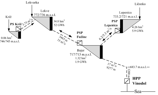

1. Introduction

This paper formulates a hydro-economic river basin model (HERBM) of a price-taking hydro generating company (GENCO, Zagreb, Croatia) which participates in a simultaneous energy and ancillary services day-ahead markets (DAMs) [1–5]. In order to successfully bid on a market, a hydro GENCO first needs to determine energy and ancillary services marginal cost curves. Since the direct cost of energy generation for a hydro GENCO is virtually zero compared to a fossil fuel GENCOs, consequently creating a marginal cost curve is more complicated compared with finding a generation cost curve first derivative for a fossil fuel GENCO. This paper will tackle this problem, and propose easy to implement linear formulation in a form of a constraint. In this paper an opportunity cost of water is viewed as a marginal cost of water. The idea behind the opportunity cost of water is that generating one MWh in a given hour means not being able to generate one MWh in some future hour. Therefore, for a hydro GENCO, the foregone earnings from future generation constitute the opportunity cost of current energy generation. A similar study is done in [6] where a fixed head of a hydro power plant (HPP) is considered. In one of the fundamental works, a marginal cost of water is assumed to be constant over the planning horizon [7,8]. For a more realistic approach, a water shadow price should change over the planning horizon every time the reservoir capacity constraints are reached [9,10]. This was the case in this research. A lot of work has been done in a field of bidding curve optimization models and a review of these models can be found in [11], with some early works in [12–14].

Modeling of ancillary services is specifically addressed in this research using simple linear formulation where automatic generation control (AGC) state (ramp up, ramp down, no ramp) is considered as a random variable. Detailed ancillary services models are important in order to encourage competitiveness and introduction of new ancillary services providers which consequently results in higher penetration of renewable energy sources (RES) particularly wind [15–17].

In a short-term planning most of the parameters are usually considered as known and the resulting models are deterministic [18,19]. In this paper a stochastic short-term planning model is presented, which enables implementation of a risk measure. It is particularly convenient to use a conditional-value-at-risk (CVaR), a relatively new risk measure introduced in [20]. CVaR is a coherent measure of risk [21,22] which is important for the successful representation of real life occurring risks and for implementation in convex optimization problems [23]. This paper analyzes the price-taker hydro GENCO which participates simultaneously in energy and ancillary services DAMs. This paper contributes to the previous works [7–10] with the approach which combines innovative usage of the hourly CVaR, the probability of occurrence of AGC states and the opportunity cost of water to determine the energy and ancillary services marginal cost curves and consequently to determine a bid prices for energy and ancillary services. The proposed approach is in a linear constraint form and is easy to implement in optimization problems.

Relationships between the head of the associated reservoir(s), the discharged water and the generated power is considered. Models describing these relationships are available in [24–29]. Therefore, in Section 2, the cascade hydropower system (HPS) is carefully modeled as HERBM using the mixed-integer linear programming (MILP) formulation. Afterword's the ancillary services model is formulated and the risk-constrained approach for pricing energy and ancillary services is introduced. Section 3 presents and analyzes the results on the case of HPS Vinodol (Croatia) and in Section 4 conclusions are given.

2. Problem Description and Formulation

In this chapter, hourly water marginal costs are determined. The profit maximization objective function is formulated. Hourly CVaR as a risk measure is formulated. Ancillary services model is formulated with AGC state as a discrete random variable. Probability of occurrence of AGC states are later used as a rule for redistributing the water marginal cost along the energy, the regulation and the 10 min spinning reserve. Afterwards the energy, regulation and 10 min spinning reserve marginal costs are used for determining an hourly bidding curves.

2.1. Hydro Constraints

The continuity equation of the hydro reservoirs is formulated as Equations (1) and (2). The variable defined after semicolon denotes the associated dual variable:

$$X(i,t,\mathrm{\omega })=X(i,t-1,\mathrm{\omega })+M\cdot [W(i,t,\mathrm{\omega })+\text{∑}_{j\in U}\{q(j,t-{\mathrm{\tau }}_{ij},\mathrm{\omega })+s(j,t-{\mathrm{\tau }}_{ij},\mathrm{\omega })\}-(q(i,t,\mathrm{\omega })+s(i,t,\mathrm{\omega }))]\forall i\in I,\forall t\in T,\forall \mathrm{\omega }\in \mathrm{\Omega }$$

(1)

$$\begin{array}{c}X(i,t,\mathrm{\omega })\le X_{\text{max}}(i);{\kappa }^{X_{\text{max}}}(i,t,\mathrm{\omega })\\ X(i,t,\mathrm{\omega })\ge X_{\text{min}}(i);{\upsilon }^{X_{\text{min}}}(i,t,\mathrm{\omega })\\ s(i,t,\mathrm{\omega })\ge B_{\text{min}};\forall i\in I,\forall t\in T,\mathrm{\omega }\in \mathrm{\Omega }\end{array}$$

(2)

For unit consistency, it should be noted the time periods of 1 h are considered. The τ_ij is the time delay for water transportation between reservoirs i and j.

2.2. Head Dependent Power Output

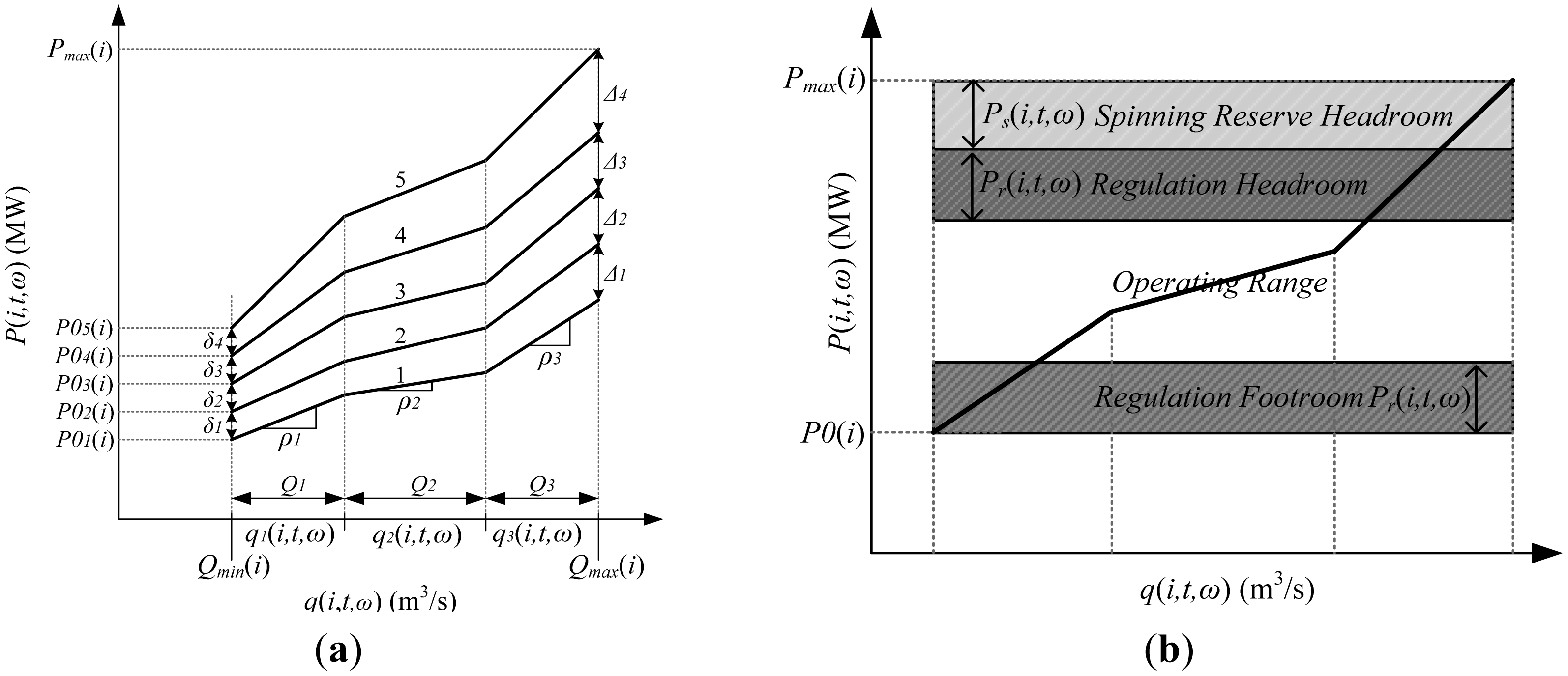
The performance curves (Figure 1) are modeled through a piecewise linear formulation of a Hill chart [30]. Non-concavities are modeled through the use of binary variables. Figure 1a shows three-piece linear performance curves.

The slope ρ is defined by HPP conversion capabilities (MWs/m³). The five performance curves are associated for the five water contents intervals. Activation of the corresponding performance curve is done by the approach presented in [31]. Unlike [32,33] the operation of HPP is not restricted to the local best efficiency points. Activation of the performance curves is modeled with Equations (3)–(6).

The performance curves are activated according to the four binary variables d₁, d₂, d₃ and d₄ in Equations (3)–(6) using the average value of stored water in certain time step t Equation (3) instead of using the final reservoir water content of the time step t [26]:

$$X_{\text{avg}}(i,t,\mathrm{\omega })=\frac{X(i,t,\mathrm{\omega })+X(i,t-1,\mathrm{\omega })}{2}\forall i\in I,\forall t\in T,\forall \mathrm{\omega }\in \mathrm{\Omega }$$

(3)

$$X_{\text{avg}}(i,t,\mathrm{\omega })\ge X_1(i)\cdot [d_1(i,t,\mathrm{\omega })-d_2(i,t,\mathrm{\omega })]+X_2(i)\cdot [d_2(i,t,\mathrm{\omega })–d_3(i,t,\mathrm{\omega })]+X_3(i)\cdot [d_3(i,t,\mathrm{\omega })-d_4(i,t,\mathrm{\omega })]+X_4(i)\cdot d_4(i,t,\mathrm{\omega }),\forall i\in I,\forall t\in T,\forall \mathrm{\omega }\in \mathrm{\Omega }$$

(4)

$$\begin{array}{l}{X}_{\text{avg}}\le X_{\text{max}}(i)\cdot d_4(i,t,\mathrm{\omega })+X_1(i)\cdot [1–d_1(i,t,\mathrm{\omega })]+X_2(i)\cdot [d_1(i,t,\mathrm{\omega })-d_2(i,t,\mathrm{\omega })]\hfill \\ +X_3(i)\cdot [d_2(i,t,\mathrm{\omega })-d_3(i,t,\mathrm{\omega })]+X_4(i)\cdot [d_3(i,t,\mathrm{\omega })-d_4(i,t,\mathrm{\omega })],\forall i\in I,\forall t\in T,\forall \mathrm{\omega }\in \mathrm{\Omega }\hfill \end{array}$$

(5)

$$\begin{array}{c}{d}_1(i,t,\mathrm{\omega })\ge d_2(i,t,\mathrm{\omega })\\ d_2(i,t,\mathrm{\omega })\ge d_3(i,t,\mathrm{\omega })\\ d_3(i,t,\mathrm{\omega })\ge d_4(i,t,\mathrm{\omega }),\forall i\in I,\forall t\in T,\forall \mathrm{\omega }\in \mathrm{\Omega }\end{array}$$

(6)

Depending on the binary variables d₁, d₂, d₃ and d₄ combination the corresponding performance curve will activate. For instance if the binary variables are set to 1, 0, 0, 0 the performance curve Equation (8) is activated, if the binary variables are 1, 1, 1, 0 then the curve Equation (10) is activated and, etc. Formulation of the performance curves is shown in Equations (7)–(13).

$$\begin{array}{c}P(i,t,\mathrm{\omega })-P{0}_1(i)\cdot w(i,t,0,\mathrm{\omega })-\text{∑}_{b=1}^3{q}_u(i,t,b,\mathrm{\omega })\cdot \mathrm{\rho }(i,b)\\ -P_{\text{max}}(i)\cdot [d_1(i,t,\mathrm{\omega })+d_2(i,t,\mathrm{\omega })+d_3(i,t,\mathrm{\omega })+d_4(i,t,\mathrm{\omega })]\le 0\\ P(i,t,\mathrm{\omega })-P{0}_1(i)\cdot w(i,t,0,\mathrm{\omega })-\text{∑}_{b=1}^3{q}_u(i,t,b,\mathrm{\omega })\cdot \mathrm{\rho }(i,b)\\ +P_{\text{max}}(i)\cdot [d_1(i,t,\mathrm{\omega })+d_2(i,t,\mathrm{\omega })+d_3(i,t,\mathrm{\omega })+d_4(i,t,\mathrm{\omega })]\ge 0,\forall i\in I,\forall t\in T,\forall \mathrm{\omega }\in \mathrm{\Omega }\end{array}$$

(7)

$$\begin{array}{c}P(i,t,\mathrm{\omega })-P{0}_2(i)\cdot w(i,t,0,\mathrm{\omega })-\text{∑}_{b=1}^3{q}_u(i,t,b,\mathrm{\omega })\cdot \mathrm{\rho }(i,b)\\ -P_{\text{max}}(i)\cdot [1-d_1(i,t,\mathrm{\omega })+d_2(i,t,\mathrm{\omega })+d_3(i,t,\mathrm{\omega })+d_4(i,t,\mathrm{\omega })]\le 0\\ P(i,t,\mathrm{\omega })-P{0}_2(i)\cdot w(i,t,0,\mathrm{\omega })-\text{∑}_{b=1}^3{q}_u(i,t,b,\mathrm{\omega })\cdot \rho (i,b)\\ +P_{\text{max}}(i)\cdot [1-d_1(i,t,\mathrm{\omega })+d_2(i,t,\mathrm{\omega })+d_3(i,t,\mathrm{\omega })+d_4(i,t,\mathrm{\omega })]\ge 0,\forall i\in I,\forall t\in T,\forall \mathrm{\omega }\in \mathrm{\Omega }\end{array}$$

(8)

$$\begin{array}{c}P(i,t,\mathrm{\omega })-P{0}_3(i)\cdot w(i,t,0,\mathrm{\omega })-\text{∑}_{b=1}^3{q}_u(i,t,b,\mathrm{\omega })\cdot \mathrm{\rho }(i,b)\\ -P_{\text{max}}(i)\cdot [2-d_1(i,t,\mathrm{\omega })-d_2(i,t,\mathrm{\omega })+d_3(i,t,\mathrm{\omega })+d_4(i,t,\mathrm{\omega })]\le 0\\ P(i,t,\mathrm{\omega })-P{0}_3(i)\cdot w(i,t,0,\mathrm{\omega })-\text{∑}_{b=1}^3{q}_u(i,t,b,\mathrm{\omega })\cdot \mathrm{\rho }(i,b)\\ +P_{\text{max}}(i)\cdot [2-d_1(i,t,\mathrm{\omega })-d_2(i,t,\mathrm{\omega })+d_3(i,t,\mathrm{\omega })+d_4(i,t,\mathrm{\omega })]\ge 0,\\ \forall i\in I,\forall t\in T,\forall \mathrm{\omega }\in \mathrm{\Omega }\end{array}$$

(9)

$$\begin{array}{c}P(i,t,\mathrm{\omega })-P{0}_4(i)\cdot w(i,t,0,\mathrm{\omega })-\text{∑}_{b=1}^3{q}_u(i,t,b,\mathrm{\omega })\cdot \mathrm{\rho }(i,b)\\ -P_{\mathit{\text{max}}}(i)\cdot [3-d_1(i,t,\mathrm{\omega })-d_2(i,t,\mathrm{\omega })-d_3(i,t,\mathrm{\omega })+d_4(i,t,\mathrm{\omega })]\le 0\\ P(i,t,\mathrm{\omega })-P{0}_4(i)\cdot w(i,t,0,\mathrm{\omega })-\text{∑}_{b=1}^3{q}_u(i,t,b,\mathrm{\omega })\cdot \mathrm{\rho }(i,b)\\ +P_{\text{max}}(i)\cdot [3-d_1(i,t,\mathrm{\omega })-d_2(i,t,\mathrm{\omega })-d_3(i,t,\mathrm{\omega })+d_4(i,t,\mathrm{\omega })]\ge 0,\\ \forall i\in I,\forall t\in T,\forall \mathrm{\omega }\in \mathrm{\Omega }\end{array}$$

(10)

$$\begin{array}{c}P(i,t,\mathrm{\omega })-P{0}_5(i)\cdot w(i,t,0,\mathrm{\omega })-\text{∑}_{b=1}^3{q}_u(i,t,b,\mathrm{\omega })\cdot \mathrm{\rho }(i,b)\\ -P_{\text{max}}(i)\cdot [4-d_1(i,t,\mathrm{\omega })-d_2(i,t,\mathrm{\omega })-d_3(i,t,\mathrm{\omega })-d_4(i,t,\mathrm{\omega })]\le 0\\ P(i,t,\mathrm{\omega })-P{0}_5(i)\cdot w(i,t,0,\mathrm{\omega })-\text{∑}_{b=1}^3{q}_u(i,t,b,\mathrm{\omega })\cdot \mathrm{\rho }(i,b)\\ +P_{\text{max}}(i)\cdot [4-d_1(i,t,\mathrm{\omega })-d_2(i,t,\mathrm{\omega })-d_3(i,t,\mathrm{\omega })-d_4(i,t,\mathrm{\omega })]\ge 0,\\ \forall i\in I,\forall t\in T,\forall \mathrm{\omega }\in \mathrm{\Omega }\end{array}$$

(11)

$$\begin{array}{c}q(i,t,b,\mathrm{\omega })\le Q_{\text{max}}(i,b)\cdot w(i,t,b-1\mathrm{\omega })\\ \begin{array}{cc}q(i,t,b,\mathrm{\omega })\ge Q_{\text{max}}(i,b)\cdot w(i,t,b,\mathrm{\omega }),& \forall b\in B,\forall i\in I,\forall t\in T,\forall \mathrm{\omega }\in \mathrm{\Omega }\end{array}\end{array}$$

(12)

$$q(i,t,\mathrm{\omega })=\text{∑}_{b=1}^{3}q(i,t,b,\mathrm{\omega })+Q_{\text{min}}(i)\cdot w(i,t,0,\mathrm{\omega })$$

(13)

2.3. Day-Ahead Market

In this work the hydro GENCO participates in the simultaneous energy and ancillary service DAM. Markets are considered competitive enough to assume the analyzed GENCO is a price-taker. The 10 min spinning reserve and regulation markets are considered as the ancillary service markets. In DAM considered here the independent system operator (ISO) will commit GENCOs in a similar way as ISO did in the vertically integrated structure using security constrained unit commitment (SCUC). Suppliers submit their bids to supply the forecasted daily inelastic demand and ISO uses the bid-in costs submitted by GENCOs for each generating unit (multi-part bids that reflect start-up costs, minimum generation costs, capacity offered, running costs, etc.) to minimize cost of operation and determine which units will be dispatched in how many hours and calculate the corresponding market clearing prices (MCPs) while the system security is retained The prices of energy and ancillary services are set at the shadow price of the market clearing constraints for the corresponding product and as a result, generating units are dispatched to maximize their profits given the prices of energy and ancillary services. Such market design is incentive for a competitive generator to select as a weakly dominating strategy bidding the actual generation cost and operation parameters. DAM market modeled here is assumed to be similar to New York DAM (New York Independent System Operator—NYISO) [34].

2.4. Ancillary Services

Besides participating in energy DAM, GENCO participates in the 10 min spinning reserve DAM and the regulation DAM. Ancillary services markets are country-dependent and a review of these markets designs is available in [35]. An HPP parameter important for modeling frequency regulation services is the maximum sustain ramp rate parameter (MSR [MW/min]) which defines how much unit can increase (MSR up) or decrease (MSR down) its output in time period of minute. The regulation and spinning reserve services are modeled based on the approach presented in [36], with the improvements Equations (16)–(21) regarding probability of occurrence of particular AGC state. When GENCO participates in the regulation DAM, the following AGC states may occur:

• Regulation-up: HPP power output increases. GENCO earns on available regulation capacity P_r(t,ω) priced at π_r(t,ω) and on electricity produced for regulation service E_r(t,ω) priced at π_spot(t,ω) in a time period t and a price scenario ω. Probability of being in this state is p_rup(t,ω).

• Regulation-down: HPP power output decreases. GENCO earns on available regulation capacity P_r(t,ω) priced at π_r(t,ω), GENCO does not repay nor gets repaid for energy decreased priced at π_spot(t,ω) in a time period t and a price scenario ω. Probability of being in this state is p_rdown(t,ω)

• No-regulation: There is no change in HPP power output. GENCO earns on available regulation capacity P_r(t,ω) priced at π_r(t,ω ) in a time period t and a price scenario ω. Probability of being in this state is 1 − p_rup(t,ω) − p_rdown(t,ω).

When GENCO commits in the 10 min spinning reserve DAM the following AGC states may occur:

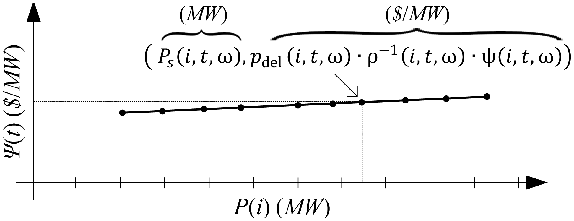
• Reserve-up: HPP power output increases. GENCO earns on 10 min spinning reserve capacity P_s(t,ω) available for increase of power output priced at π_s(t,ω) in time period t and price scenario ω. Also GENCO earns on electricity produced for spinning reserve service E_s(t) priced at π_spot(t) in a time period t and a price scenario ω. Probability of being in this state is p_del(t,ω).

• Reserve-neutral: There is no change in HPP power output. GENCO earns on 10 min spinning reserve capacity P_s(t,ω) available for increase of power output priced at π_s(t,ω) in a time period t and a price scenario ω . Probability of being in this state is 1 − p_del(t,ω).

The operating range of HPP when committed in the regulation and the 10 min spinning reserve DAM is defined with Equation (14) and is depicted in Figure 1b. A review of ancillary services models is available in [36–39]:

$$\begin{array}{l}{P}_e(i,t,\mathrm{\omega })\le P_{\text{max}}(i)-P_r(i,t,\mathrm{\omega })-P_s(i,t,\mathrm{\omega });{\kappa }^{P_{\text{max}}}(i,t,\mathrm{\omega })\hfill \\ P_e(i,t,\mathrm{\omega })\ge P_0(i)+P_r(i,t,\mathrm{\omega });{\upsilon }^{P_0}(i,t,\mathrm{\omega }),\forall i\in I,\forall t\in T,\forall \mathrm{\omega }\in \mathrm{\Omega }\hfill \end{array}$$

(14)

For the regulation capacity P_r(i,t,ω), the value indicates the ability to move both up and down and requires both headroom and footroom, while provision of the spinning reserve P_s(i,t,ω) requires headroom but not footroom, meaning HPP cannot provide energy at its maximum output level but can run at minimum output level. Practical implementation of Equation (14) is shown in Equation (15) and is depicted in Figure 1:

$$\begin{array}{l}{P}_e(i,t,\mathrm{\omega })\le P_{\text{max}}(i)+{\mathrm{\Delta }}_1(i)\cdot (d_1(i,t,\mathrm{\omega })-1)\hfill \\ +{\mathrm{\Delta }}_2(i)\cdot (d_2(i,t,\mathrm{\omega })-1)+{\mathrm{\Delta }}_3(i)\cdot (d_3(i,t,\mathrm{\omega })-1)\hfill \\ +{\mathrm{\Delta }}_4(i)\cdot (d_4(i,t,\mathrm{\omega })-1))-P_r(i,t,\mathrm{\omega })-P_s(i,t,\mathrm{\omega })\hfill \\ P_e(i,t,\mathrm{\omega })\ge P{0}_5(i)+{\mathrm{\delta }}_1(i)\cdot (d_1(i,t,\mathrm{\omega })-1)\hfill \\ +{\mathrm{\delta }}_2(i)\cdot (d_2(i,t,\mathrm{\omega })-1)+{\mathrm{\delta }}_3(i)\cdot (d_3(i,t,\mathrm{\omega })-1)\hfill \\ +{\mathrm{\delta }}_4(i)\cdot (d_4(i,t,\mathrm{\omega })-1)+P_r(i,t,\mathrm{\omega }),\forall i\in I,\forall t\in T,\forall \mathrm{\omega }\in \mathrm{\Omega }\hfill \end{array}$$

(15)

Expected electricity produced when committed in the simultaneous energy, regulation and spinning reserve DAM in a time period t and a price scenario ω Equation (16).

$$\begin{array}{l}\mathbf{\text{E}}[E(i,t,\mathrm{\omega })]=E_e(i,t,\mathrm{\omega })+E_r(i,t,\mathrm{\omega })+E_s(i,t,\mathrm{\omega })\hfill \\ =P_e(i)+\left(p_{\text{rup}}(t,\mathrm{\omega })-p_{r\text{down}}(t,\mathrm{\omega })\right)\cdot P_r(i,t,\mathrm{\omega })\hfill \\ +p_{\text{del}}(t,\mathrm{\omega })\cdot P_s(i,t,\mathrm{\omega }),\forall i\in I,\forall t\in T,\forall \mathrm{\omega }\in \mathrm{\Omega }\hfill \end{array}$$

(16)

Multiplying the ancillary service capacities P_r(i,t,ω) and P_s(i,t,ω) with the probabilities p_del(t,ω),p_rup(t,ω) and p_rdown(t,ω) defines the energy produced for particular ancillary service in a time step t and a price scenario to Equations (18)–(20).

The probability matrix p_AGC (17) of size ℝ^T_max × ℝ^Ω_max represents the probability of occurrence of the particular automatic generation control (AGC) state the Regulation-up state the Regulation-down state and the Reserve-up state for ∀t ∈ T and ∀ω ∈ Ω. The matrix can be obtained statistically by a GENCO who has a history on offering ancillary services, whether they are committed obligatory, bilaterally or on the auction market, since this matrix is solely defined by technical features of frequency regulation zone:

$$p_{\text{AGC}}=\begin{array}{cc}\left(\begin{array}{ccccc}p(1,1)& \cdots & p(1,\mathrm{\omega })& \cdots & p(1,{\mathrm{\Omega }}_{\text{max}})\\ ⋮& \ddots & ⋮& \ddots & ⋮\\ p(t,1)& \cdots & p(t,\mathrm{\omega })& \cdots & p(t,{\mathrm{\Omega }}_{\text{max}})\\ ⋮& \ddots & ⋮& \ddots & ⋮\\ p(T_{\text{max}},1)& \cdots & p(T_{\text{max}},\mathrm{\omega })& \cdots & p(T_{\text{max}},{\mathrm{\Omega }}_{\text{max}})\end{array}\right),& \forall \text{AGC}\in \{\mathit{\text{rup}},\mathit{\text{rdown}},\mathit{\text{del}}\}\end{array}$$

(17)

Electricity produced for the energy market Equation (18):

$$E_e(i,t,\mathrm{\omega })=P_e(i,t,\mathrm{\omega }),\forall i\in I,\forall t\in T,\forall \mathrm{\omega }\in \mathrm{\Omega }$$

(18)

Electricity produced for the regulation service Equation (19):

$$E_r(i,t,\mathrm{\omega })=\left(p_{\text{rup}}(t,\mathrm{\omega })-p_{r\text{down}}(t,\mathrm{\omega })\right)\cdot P_r(i,t,\mathrm{\omega }),\forall i\in I,\forall t\in T,\forall \mathrm{\omega }\in \mathrm{\Omega }$$

(19)

Electricity produced for the spinning reserve service Equation (20):

$$E_s(i,t,\mathrm{\omega })=p_{\text{del}}(t,\mathrm{\omega })\cdot P_s(i,t,\mathrm{\omega }),\forall i\in I,\forall t\in T,\forall \mathrm{\omega }\in \mathrm{\Omega }$$

(20)

Expected electricity produced is equal to the performance curve Equations (3)–(12) in all time intervals Equation (21):

$$\mathbf{\text{E}}[E(i,t,\mathrm{\omega })]=P(i,t,\mathrm{\omega }),\forall i\in I,\forall t\in T,\forall \mathrm{\omega }\in \mathrm{\Omega }$$

(21)

Ramp rate limits Equation (22):

$$\begin{array}{l}P(i,t,\mathrm{\omega })-P(i,t-1,\mathrm{\omega })\le UP(i)\hfill \\ P(i,t-1,\mathrm{\omega })-P(i,t,\mathrm{\omega })\le DR(i),\forall i\in I,\forall t\in T,\forall \mathrm{\omega }\in \mathrm{\Omega }\hfill \end{array}$$

(22)

The maximum regulation capacity that can be offered is calculated as the MSR times five min Equation (23). The 10 min spinning capacity is defined as the MSR times ten min Equation (24).

$$0\le P_r(i,t,\mathrm{\omega })\le 5\times \text{MSR}(i),\forall i\in I,\forall t\in T,\forall \mathrm{\omega }\in \mathrm{\Omega }$$

(23)

$$0\le P_s(i,t,\mathrm{\omega })\le 10\times \text{MSR}(i),\forall i\in I,\forall t\in T,\forall \mathrm{\omega }\in \mathrm{\Omega }$$

(24)

2.5. Random Variable: Energy and Ancillary Services MCPs

The set Ω will represent future states of knowledge, and the single element ω will define a one future state, meaning ω ∈ Ω The set Ω will have a mathematical structure of probability space with probability measure p for comparing the likelihood of the future states ω.

The discrete random variable π as shown in Equation (25) will represent random daily price series, and is defined with Π : Ω → A, where A ⊆ ℝ^Tmax since probability won't be defined on each element of ℝ^Tmax vector space.

The probability of particular daily price scenario of market m Π_m(ω) ∈ A is defined as Equation (26):

$$\begin{array}{l}{\mathrm{\Pi }}_m=\left(\begin{array}{ccccc}\mathrm{\pi }(1)& \cdots & \mathrm{\pi }(\mathrm{\omega })& \cdots & \mathrm{\pi }({\mathrm{\Omega }}_{\text{max}})\\ p(1)& \cdots & p(\mathrm{\omega })& \cdots & p({\mathrm{\Omega }}_{\text{max}})\end{array}\right),\forall m\in \left\{e,r,s,\text{spot}\right\}\hfill \\ \text{where},\left\{\mathrm{\omega }\in \mathrm{\Omega }:{\mathrm{\Pi }}_m(\mathrm{\omega })=(\mathrm{\pi }(1),\dots ,\mathrm{\pi }(t),\dots ,\mathrm{\pi }(T_{\text{max}}))\right\},\forall m\in \left\{e,r,s,\text{spot}\right\}\hfill \end{array}$$

(25)

$$p\{{\mathrm{\Pi }}_m(\mathrm{\omega })\}=P(\mathrm{\omega }\in \mathrm{\Omega }:{\mathrm{\Pi }}_m(\mathrm{\omega })\in A)=p(\mathrm{\omega }),\forall m\in \{e,r,s,\text{spot}\}$$

(26)

Finite number of future states are observed, ω∈Ω ⊆ ℕ. The random variable Equation (25) is defined for energy and ancillary service DAM. Moreover, it can be shown that the distribution of hourly prices is approximately lognormal [33]. Thus resulting random variable Π_m is defined for the each time step t separately Equation (27):

$${\mathrm{\Pi }}_m=\left(\begin{array}{ccccc}\mathrm{\pi }(t,1)& \cdots & \mathrm{\pi }(t,\mathrm{\omega })& \cdots & \mathrm{\pi }(t,{\mathrm{\Omega }}_{\text{max}})\\ p(t,1)& \cdots & p(t,\mathrm{\omega })& \cdots & p(t,{\mathrm{\Omega }}_{\text{max}})\end{array}\right),\forall m\in \{e,r,s,\text{spot}\}$$

(27)

2.6. Risk Measure

An easy way to incorporate a risk into linear model is to use CVaR [16] as a measure of risk. β-CVaR is defined as an average loss of a 1-β worst scenarios, thus called tail loss (Figure 2a). α-CVaR (Figure 2b) is an average profit in worst 1-α (i.e., 15%) scenarios and α-VaR is minimal profit which GENCO can expect in rest α (i.e., 85%) scenarios.

CVaR is a coherent measure of risk, meaning CVaR has properties of convexity, monotonicity, closedness, positive homogeneity, subadditivity and translation invariance [20–23]. In the next section α-VaR and α-CVaR are formulated using the profit PDF as depicted in Figure 2b.

Both α-VaR and α-CVaR can be calculated by solving an elementary optimization problem of convex type in one dimension. For this purpose the special function Equation (28) is formulated:

$$\begin{array}{l}{F}_{\mathrm{\alpha }}(\text{Variables},\mathrm{\zeta })=\mathrm{\zeta }-\frac{1}{1-\mathrm{\alpha }}\text{∑}_{\mathrm{\omega }=1}^{{\mathrm{\Omega }}_{\text{max}}}p(\mathrm{\omega })\cdot {\left[\mathrm{\zeta }-\text{∑}_{t=1}^T\text{Profit}(t,\mathrm{\omega })\right]}^{+}\hfill \\ \text{where},{\left[\mathrm{\zeta }-{\text{∑}}_{t=1}^T\text{Profit}(t,\mathrm{\omega })\right]}^{+}=max\{0,\mathrm{\zeta }-{\text{∑}}_{t=1}^T\text{Profit}(t,\mathrm{\omega })\}\hfill \end{array}$$

(28)

When maximizing Equation (29) over all variables defined in the model, Equations (30) and (31) are obtained:

$$\underset{(\text{Variables},\mathrm{\zeta })\in {ℝ}^{\text{No. of var}}\times ℝ}{max}{F}_{\mathrm{\alpha }}(\text{Variables},\mathrm{\zeta })$$

(29)

$$\mathrm{\alpha }‐\text{CVaR}=F_{\mathrm{\alpha }}({\text{Variables}}^{*},{\mathrm{\zeta }}^{*})$$

(30)

$$\mathrm{\alpha }‐\text{VaR}={\mathrm{\zeta }}^{*}$$

(31)

where the Variables denotes all the variables defined in nomenclature. The variable ζ is shown separately only to point out its importance. In Equations (28)–(31) a risk measure is expressed as a daily value.

Generally, when the daily CVaR is used, the risk will average out throughout the day, and this is not desirable as, especially in a case of a major contingency in particular hour–this can result in unpredictable values of the daily CVaR. Consequently, the hourly α-VaR(t) and the hourly α-CVaR(t) are formulated using the hourly special function F_α(Variables_t, ζ(t)) over all (Variables_t, ζ(t)) ∈ ℝ^{No.of var in step t} × ℝ.

Since objective function is already defined, the special function is thus brought in the optimization problem in a form of the constraint Equation (32):

$$F_{\mathrm{\alpha }}({\mathit{\text{Variables}}}_t,\mathrm{\zeta }(t))\ge \mathit{\text{minCVaR}}(t)\forall t\in T$$

(32)

where the Variables_t denotes all the variables defined in nomenclature in a time step t. The variable ζ(t) is the hourly value.

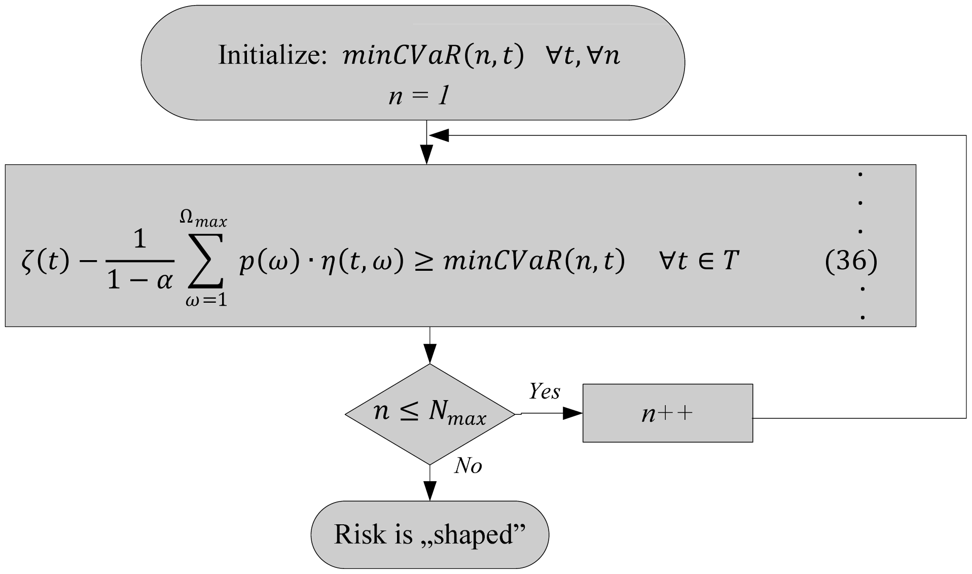
When implementing the constraint Equation (32), the risk is “shaped” using the profit tolerance minCVaR(t) ∀t ∈ T. When the set of profit tolerances minCVaR(n, t), ∀n ∈ N is introduced in the optimization model and the requirement Equation (33) is valid, then Equations (34)–(36) is used to shape the risk with CVaR (Figure 3):

$$\text{minCVaR}(n-1,t)<\text{minCVaR}(n,t)<\text{minCVaR}(n+1,t)\forall t\in T,\forall n\in N$$

(33)

The linear formulation of Equation (32), defined using indexed assignment is used in the model Equations (34)–(36):

$$\eta (t,\mathrm{\omega })\ge 0\forall t\in T,\forall \mathrm{\omega }\in \mathrm{\Omega }$$

(34)

$$\mathrm{\eta }(t,\mathrm{\omega })\ge \text{Profit}(t,\mathrm{\omega })-\mathrm{\zeta }(t)\forall t\in T,\forall \mathrm{\omega }\in \mathrm{\Omega }$$

(35)

$$\mathrm{\zeta }(t)-\frac{1}{1-\mathrm{\alpha }}\text{∑}_{\mathrm{\omega }=1}^{{\mathrm{\Omega }}_{\text{max}}}p(\mathrm{\omega })\cdot \mathrm{\eta }(t,\mathrm{\omega })\ge \text{minCVaR}(n,t)\forall t\in T$$

(36)

2.7. Objective Function

GENCO's objective function is maximal expected profit (37). GENCO can justify optimization of the expected profit by the law of large numbers because it gives an optimal decision on average. However, because of the variability of the input data, the average of the first few results may be very bad and it does not help that the decisions were optimal on average. For these reasons, quantitative models of risk and risk aversion are needed.

GENCO's profit in a time step t of a price scenario ω (37):

$$\begin{array}{l}\text{Profit}(t,\mathrm{\omega })=\text{∑}_{i\in I}[{\mathrm{\Pi }}_e(t,\mathrm{\omega })\cdot E_e(i,t,\mathrm{\omega })+{\mathrm{\Pi }}_{\text{spot}}(t,\mathrm{\omega })\cdot E_r(i,t,\mathrm{\omega })+{\mathrm{\Pi }}_r(t,\mathrm{\omega })\cdot P_r(i,t,\mathrm{\omega })\hfill \\ +{\mathrm{\Pi }}_{\text{spot}}(t,\mathrm{\omega })\cdot E_s(i,t,\mathrm{\omega })+{\mathrm{\Pi }}_s(t,\mathrm{\omega })\cdot P_s(i,t,\mathrm{\omega })]\cdot \hfill \end{array}$$

(37)

Objective function is an expected profit of the planning horizon T_max Equation (38):

$$\text{Profit}=\text{∑}_{\mathrm{\omega }=1}^{\mathrm{\Omega }}p(\mathrm{\omega })\cdot \text{∑}_{t=1}^T\text{Profit}(t,\mathrm{\omega })$$

(38)

2.8. Pricing of Energy and Ancillary Services

Shadow prices of the HERBM constrains are analyzed Equation (39). Shadow price represents change per unit of constraint, in the objective value of the optimal solution, i.e., marginal utility when relaxing constraints by a unit value or marginal cost when strengthening a constraint:

$$({\kappa }^{X_{\text{max}}}(i,t,\mathrm{\omega }),{\upsilon }^{X_{\text{min}}}(i,t,\mathrm{\omega });{\kappa }^{P_{\text{max}}}(i,t,\mathrm{\omega }),{\upsilon }^{P_0}(i,t,\mathrm{\omega });\mathrm{\psi }(i,t,\mathrm{\omega }),\mathrm{\lambda }(i,\mathrm{\omega }))$$

(39)

The shadow prices Equation (40) are paired with the parameter unit change Equation (40) of the right-hand side (r.h.s.) of the constraints Equations (2), (14) and (42):

$$(\mathrm{\Delta }{X}_{\text{max}}(i,t,\mathrm{\omega }),-\mathrm{\Delta }{X}_{\text{min}}(i,t,\mathrm{\omega });\mathrm{\Delta }{P}_{\text{max}}(i,t,\mathrm{\omega }),-\mathrm{\Delta }{P}_0(i,t,\mathrm{\omega });\mathrm{\Delta }W(i,t,\mathrm{\omega }),\mathrm{\Delta }\zeta (i,\mathrm{\omega }))$$

(40)

The Shadow price of used water Equation (41):

$$\mathrm{\psi }(i,t,\mathrm{\omega })=\mathrm{\lambda }(i,\mathrm{\omega })+{\kappa }^{X_{\text{max}}}(i,t,\mathrm{\omega })-{\upsilon }^{X_{\text{min}}}(i,t,\mathrm{\omega })$$

(41)

The shadow price of used water ψ(i,t,ω) can also be represented by a change in the objective value, per unit change of the reservoir i water inflow ΔW(i,t,ω) in a time step t and a scenario ω. Then the amount of ΔW(i,t,ω) won't be available in the other hours of scenario ω [9]. In order to determine the marginal cost of water, the standard profit-maximizing operation problem needs to be formulated [9,10] thus Equation (42):

$$\text{∑}_{t=1}^{T_{\text{max}}}(q(i,t,\mathrm{\omega })-W(i,t,\mathrm{\omega }))\le 0;\lambda (i,\mathrm{\omega })$$

(42)

Since the water shadow price ψ(i,t,ω) is in $(\frac{\$}{{\text{m}}^3})$ it needs to be converted in ($/MWh). In order to do that conversion, coefficient ρ⁻¹(i,t,ω) is formulated to evaluate energy potential of the reservoir i in a time step t and a price scenario ω. After simulation is ended Equation (43) is obtained:

$${\mathrm{\rho }}^{-1}(i,t,\mathrm{\omega })=M\cdot \frac{q(i,t,\mathrm{\omega })}{P(i,t,\mathrm{\omega })}$$

(43)

The pairs Equations (44)–(46) are obtained for every time step t and a price scenario ω. The available water is redistributed according to rule Equation (16) consequently the energy is priced as Equation (44), the regulation as Equation (45) and the 10 min spinning reserve as Equation (46) for every time step t and the scenario ω. Afterword's for the each time step t pairs Equations (44)–(46) are ordered in ascending order according to the prices of the set Ω (Figure 4):

$$\left(P_e(i,t,\mathrm{\omega }),1-p_{\text{del}}(i,t,\mathrm{\omega })-\left(p_{\text{rup}}(i,t,\mathrm{\omega })-p_{r\text{down}}(i,t,\mathrm{\omega })\right)\cdot {\mathrm{\rho }}^{-1}(i,t,\mathrm{\omega })\cdot \mathrm{\psi }(i,t,\mathrm{\omega })\right)$$

(44)

$$\left(P_r(i,t,\mathrm{\omega }),\left(p_{\text{rup}}(i,t,\mathrm{\omega })-p_{r\text{down}}(i,t,\mathrm{\omega })\right)\cdot {\mathrm{\rho }}^{-1}(i,t,\mathrm{\omega })\cdot \mathrm{\psi }(i,t,\mathrm{\omega })\right)$$

(45)

$$\left(P_s(i,t,\mathrm{\omega }),p_{\text{del}}(i,t,\mathrm{\omega })\cdot {\mathrm{\rho }}^{-1}(i,t,\mathrm{\omega })\cdot \mathrm{\psi }(i,t,\mathrm{\omega })\right)$$

(46)

Water shadow price of one additional (m³) of water in particular hour, and one (m³) reduced from all other hours, as said represents marginal cost of producing one more (m³) or (MWh) so it is particularly convenient to use for creating a bid curve. An ancillary service DAM is another opportunity for GENCO to increase profit and it generates additional opportunity costs which are reflected as an increase of water shadow prices.

The approach for pricing energy and ancillary services is depicted on Figure 5 using flow diagram form to indicate necessary steps of the approach with reference indicating the mathematical expressions used to accomplish each step. The model is defined as a MILP problem using indexed assignments. The presented results were obtained on 3.4 GHz based processor with 8 GB RAM using CPLEX (International Business Machines Corporation, New York, NY, USA) under General Algebraic Modeling System (GAMS) [40]. However, in general terms, using the dual information from a mixed integer programming problem may not capture all the terms in the problem related to the binary variables. The Case Study in this research is considered fairly accurate, since optimality tolerance is set to 0%. This means that the solver will stop when it finds a feasible integer solution within 0% of the global optimum.

3. Example and Results

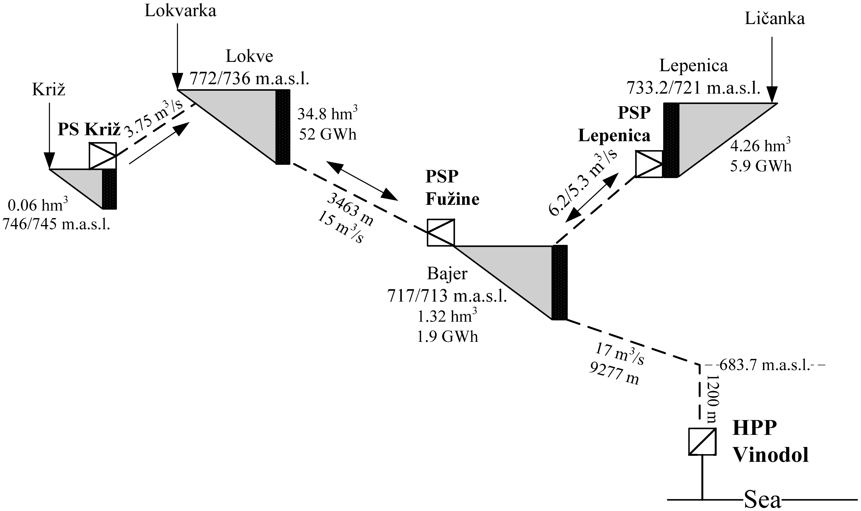
For the needs of this research HPS Vinodol (Croatia) is modeled, which consists of: four reservoirs, one pump station (PS), two pump storage hydropower plants (PSP) and one HPP (

Table 1. HPS Vinodol facilities parameters.

Reservoir	Xmax (m3)	W (m3/s)	Power Plant	Qmax (MW)	Pmax (MW)
Križ	0.06 × 106	3	PS Križ	1.1	0.34
Lokve	34.8 × 106	3	PSP Fužine	10/9	4.6/4.8
Bajer	1.32 × 106	3	HPP Vinodol	18.6	94.5
Lepenica	4.26 × 106	3	PSP Lepenica	6.2/5.3	1.14/1.25

) (Figure 6). Real HPS Vinodol is already used for frequency regulation ancillary services. Price-taker model is considered reasonably accurate since of relatively small size of HPS Vinodol compared to other participants on DAM assumed in this research.

The prices are formulated according to Equation (27) where values are normally distributed. Mean and standard deviation of prices in each time step t are statistically obtained according to Equations (47) and (48):

$$\mathrm{\mu }(t)=\frac{1}{Q_{\text{max}}}\text{∑}_{\mathrm{\omega }=1}^{{\mathrm{\Omega }}_{\text{max}}}\mathrm{\pi }(t,\mathrm{\omega })$$

(47)

$$\mathrm{\sigma }(t)=\sqrt{\frac{1}{{\mathrm{\Omega }}_{\text{max}}}\text{∑}_{\mathrm{\omega }=1}^{{\mathrm{\Omega }}_{\text{max}}}{(\mathrm{\pi }(t,\mathrm{\omega })-\mathrm{\mu }(t))}^2}$$

(48)

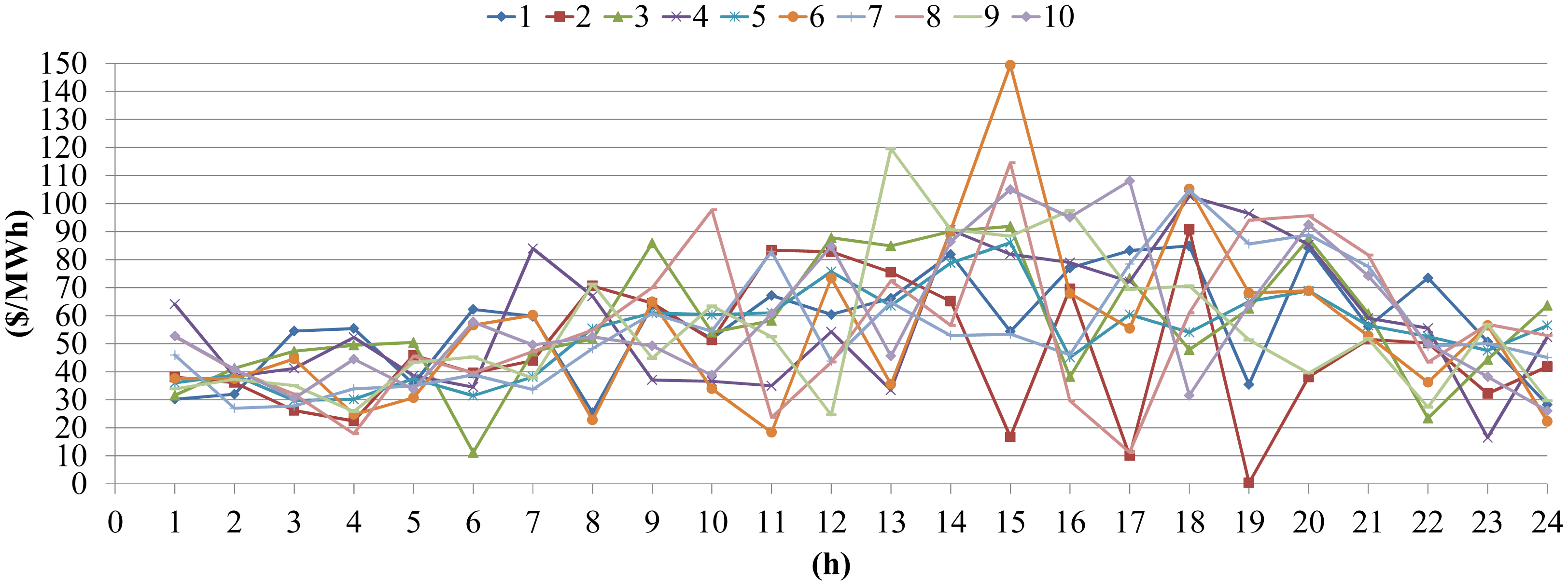
The energy and ancillary services prices are obtained from New York DAM [34], from 3 January 2011 to 5 December 2011 (337 days are observed) and descriptive statistics are calculated (

Table 2. Descriptive statistics of NYISO prices in ($/MWh).

h	Energy		Regulation		10-min		h	Energy		Regulation		10-min
	μ	σ	μ	σ	μ	σ		μ	σ	μ	σ	μ	σ
1	39.8	13.0	9.4	3.0	4.8	0.3	13	64.6	26.6	9.8	0.8	8.9	2.2
2	36.2	11.4	5.3	0.6	4.7	0.5	14	66.0	31.0	10.9	0.7	10.2	2.0
3	34.6	10.9	5.3	0.4	4.2	0.4	15	67.6	33.2	10.4	1.6	11.2	2.5
4	34.5	10.8	4.8	0.4	4.7	0.4	16	68.4	34.6	11.0	1.7	10.4	2.3
5	36.5	10.4	8.9	2.9	4.5	0.4	17	67.2	30.6	12.9	2.3	13.9	2.6
6	41.5	11.7	18.1	6.9	4.6	0.5	18	68.1	27.8	11.3	2.1	10.1	2.6
7	48.2	15.9	13.1	4.7	6.1	1.1	19	67.4	24.8	10.8	2.4	9.7	2.1
8	52.5	17.8	12.1	3.1	8.9	0.7	20	64.1	21.7	10.3	0.8	9.6	1.1
9	55.6	17.8	13.3	3.2	9.0	0.4	21	58.2	20.1	10.4	1.2	10.1	1.2
10	59.2	19.5	10.0	0.0	8.5	0.4	22	51.5	17.5	11.4	1.1	11.0	1.1
11	61.7	21.5	10.0	0.1	9.4	0.6	23	46.1	14.9	10.7	1.6	6.4	1.3
12	62.8	22.9	11.1	1.0	9.9	1.1	24	43.7	14.5	10.3	1.8	5.0	0.0

). Using pseudo-random number sampling and obtained descriptive statistics ten price scenarios (Ω_max = 10) are generated for each hour (Figure 7). The probability of occurrence p(t,ω) of the each scenario ω in the hour t is 1/Ω_max.

Observed GENCO owns HPS Vinodol. For clarity and computational effectiveness HPP Vinodol profit is maximized while rest of HPS is used for that objective. There is no significant lose in accuracy when having in mind that in GENCO's profit, HPP Vinodol profit participates with 95% or more. Probabilities are considered stationary, p_e is 100%, p_del is 3%, p_rupand p_rdown are 40% and 35% respectively [35]. The confidence level α is set to 0.85. Having in mind ancillary services requirements [41,42] and the HPP Vinodol ramp rate limits (

Table 3. Daily profit and daily risk measures α-CVaR and α-VaR for confidence level α = 0,85 expressed in dependence of hourly α-CVaR(t).

α-CVaR(t)	Profit	α-CVaR	α-VaR
0	98,193	0	0
400	97,838	9,600	14,400
800	98,162	19,100	28,500
1,380	96,959	33,120	44,037

) the problem is considered sufficiently accurate. The ramp rate limits of HPP Vinodol are as follows; MSR(up) is 255.15 MW/min, MSR(down) is 340.2 MW/min, ramping capabilities UR and DR between hours is 94.2 MW/h. The profit tolerances are minCVaR(1,t) = 0 , minCVaR(2,t) = 400 , minCVaR(3,t) = 800, and minCVaR(4,t) = 1380 for every t.

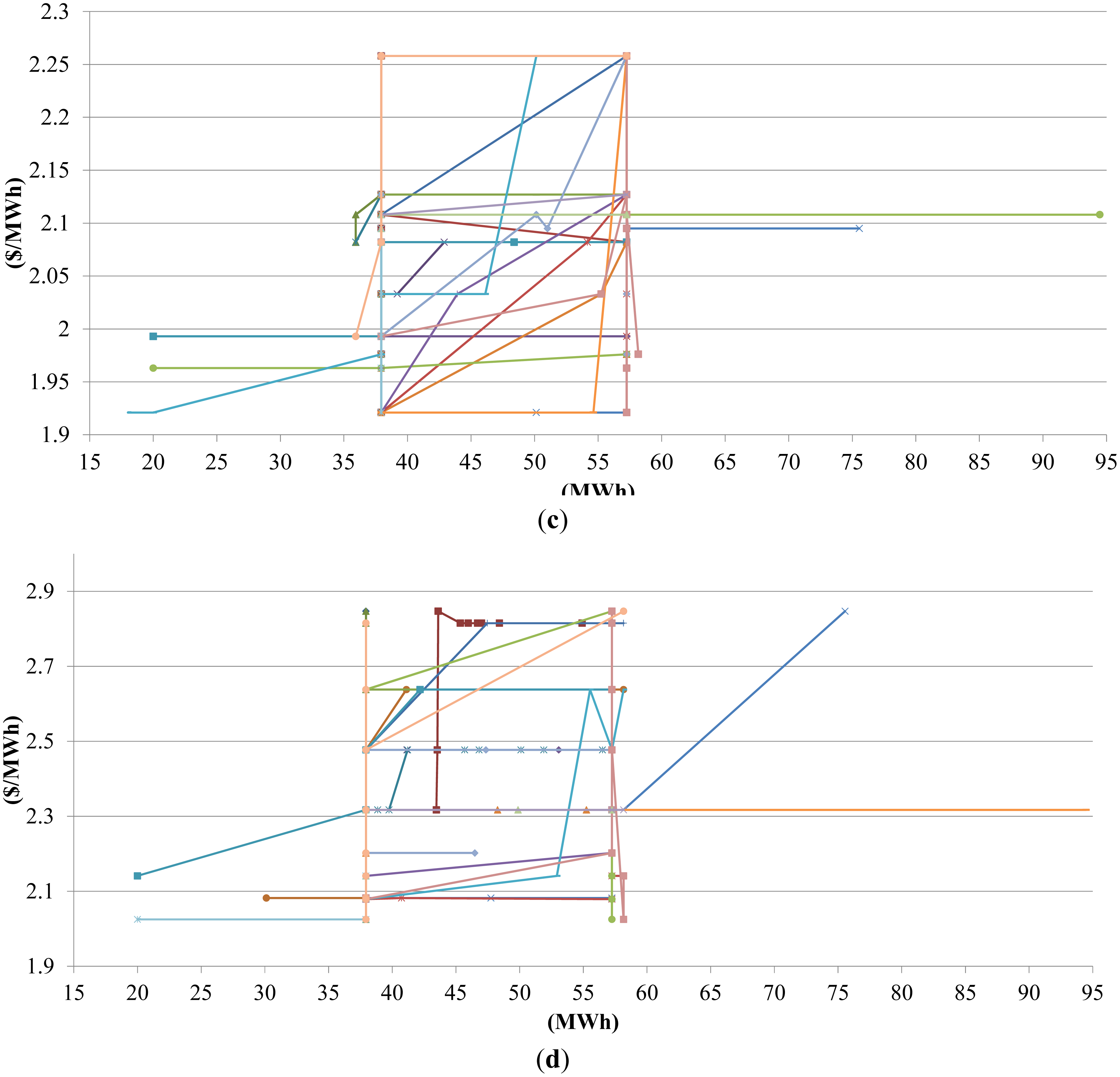
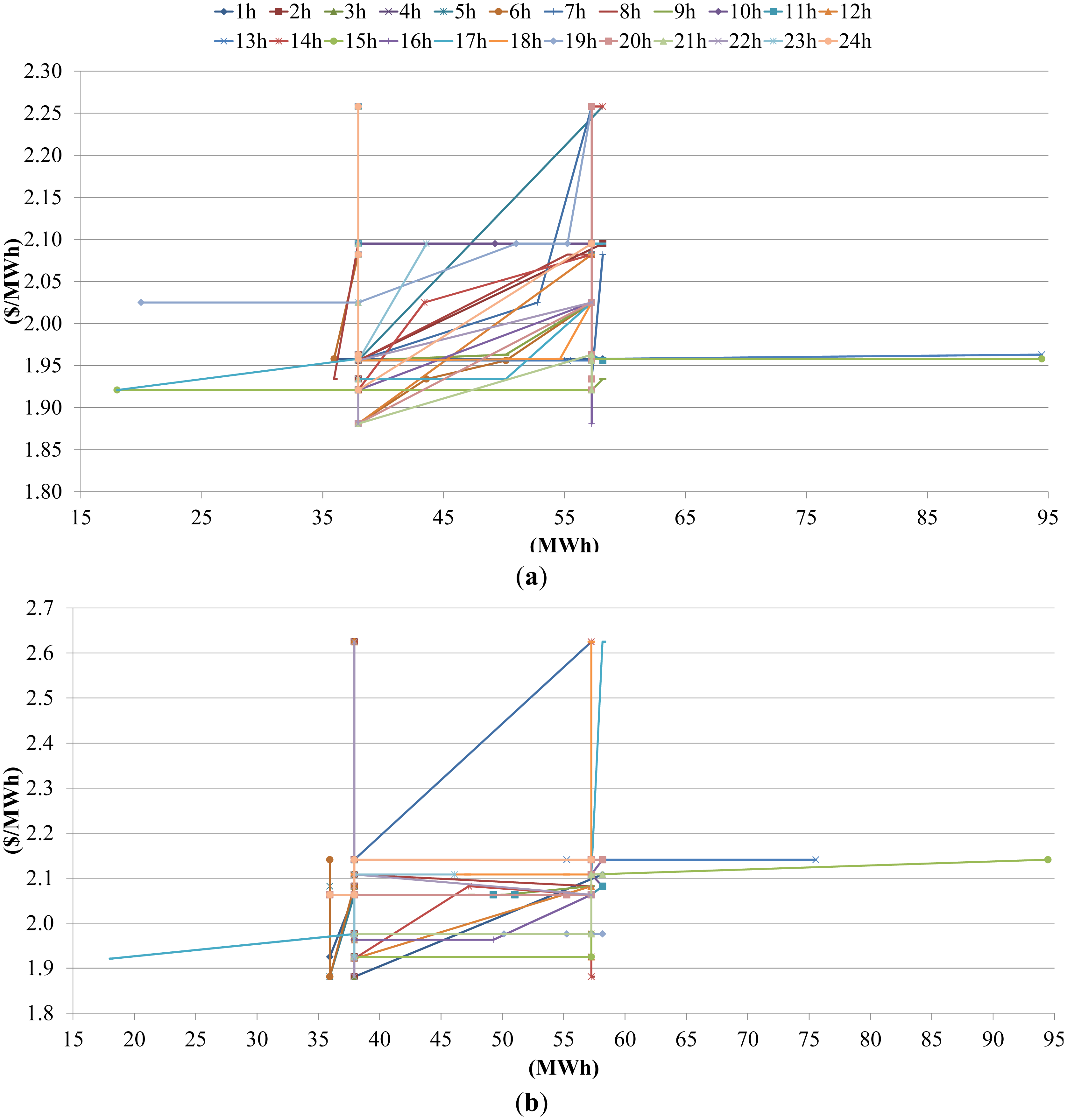
The perfectly inelastic (vertical) energy marginal cost curves here considered as bid curves are obtained for the ordinate values 38 MWh and 57 MWh (Figure 8). For the price threshold $0 and $1380 the mean shadow prices are $1.9 and $2.4, respectively. This means reducing risk costs, and these costs can be determined.

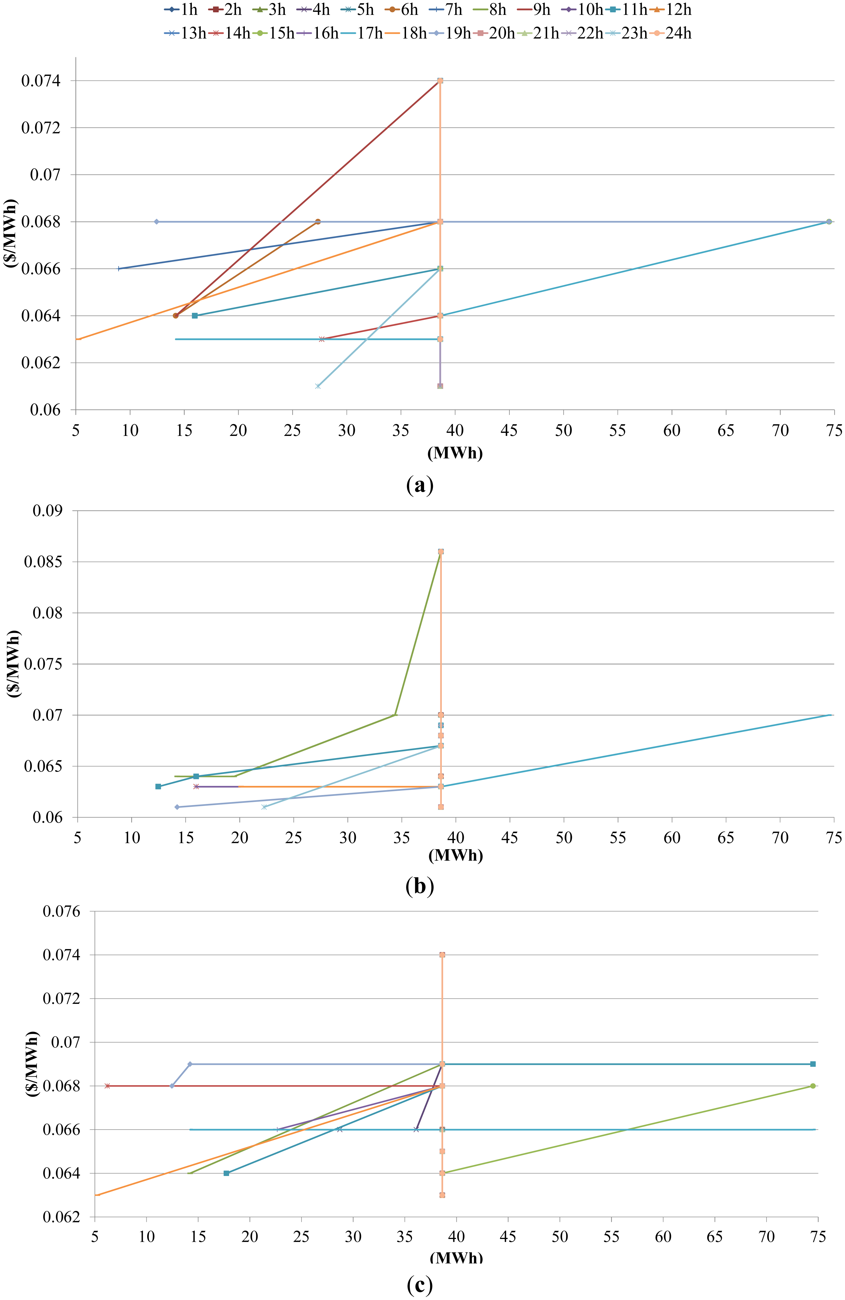
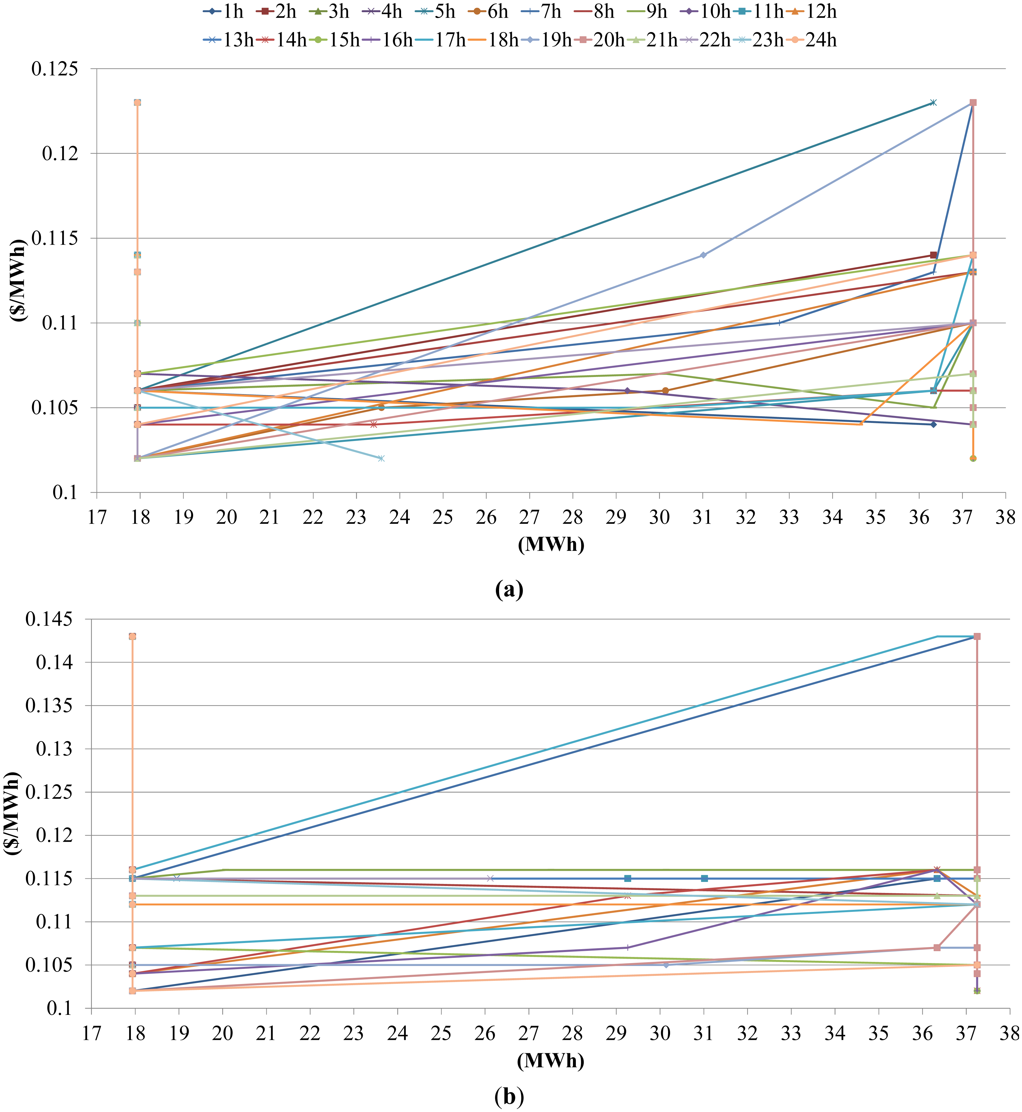
For the regulation DAM (Figure 9), the perfectly inelastic bid curves are obtained for 18 MW and 37 MW and at the same points all other bid curves are ending, reason for this is regulation headroom and footroom. For the price threshold $0 and $1′380 the mean shadow prices are $0.11 and $0.135, respectively.

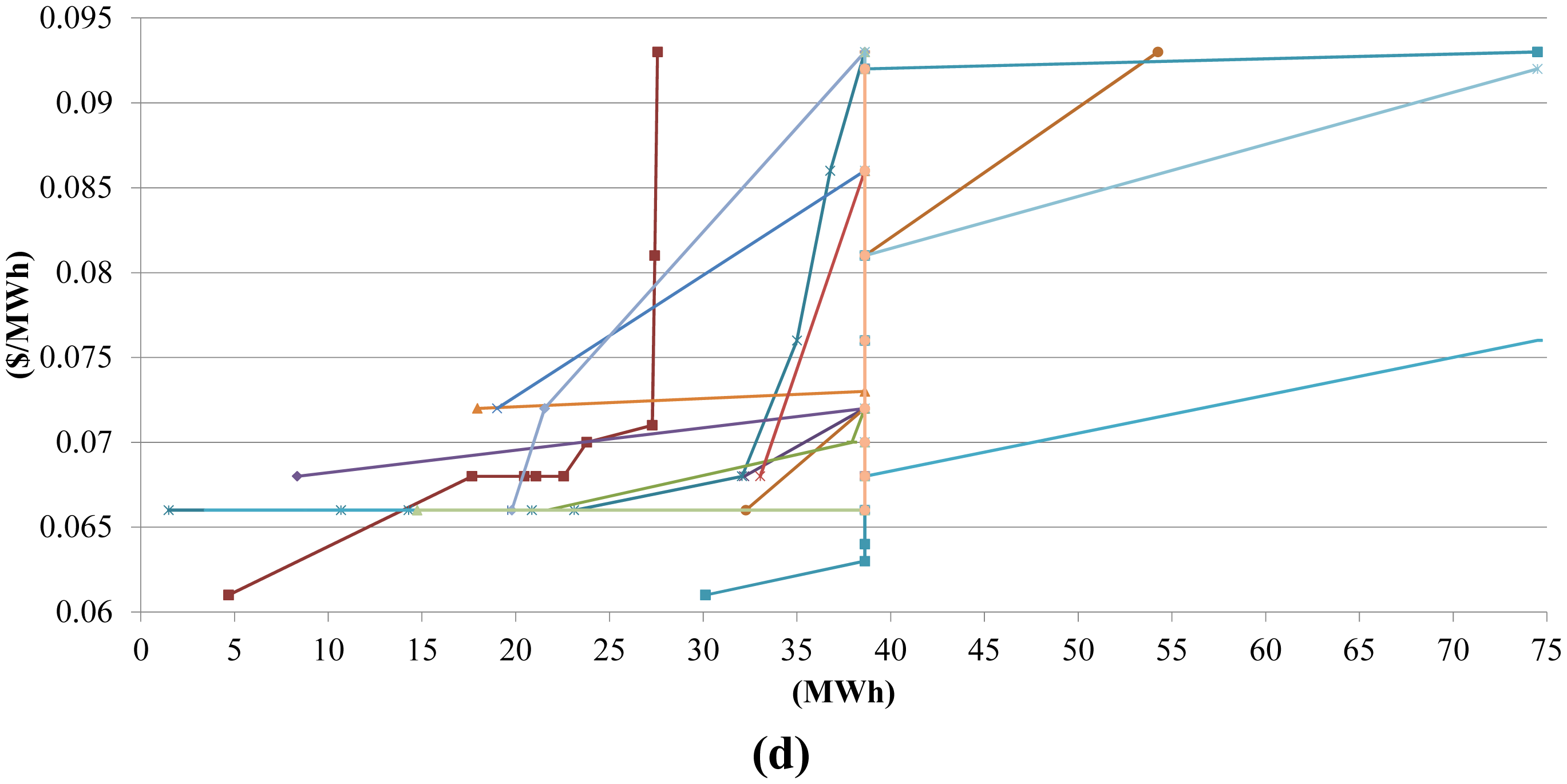
For spinning reserve DAM (Figure 10), most of the bid curves are perfectly inelastic and located around 38 MW. Optimization showed that GENCO should seek to bid certain amount of capacity. When the price threshold increases from $0 to $1380 the mean spinning reserve prices are $0.065 and $0.075, respectively.

The water shadow prices have relatively low deviation compared to DAM prices and in this research use of the simplified approach with the constant water shadow prices over the planning horizon is justified. The hourly water shadow prices also have relatively low mean value which is a result of having more than enough water with relative relationships maintained so conclusions can be given (e.g., ratio between energy and ancillary services bid prices is similar to the ratio between energy and ancillary services DAM prices). The results were not obtained for lesser amount of water to avoid long computation time. Further bid curve analysis is omitted in this work since its slope, ordinate and aspics position is highly determined by input parameters.

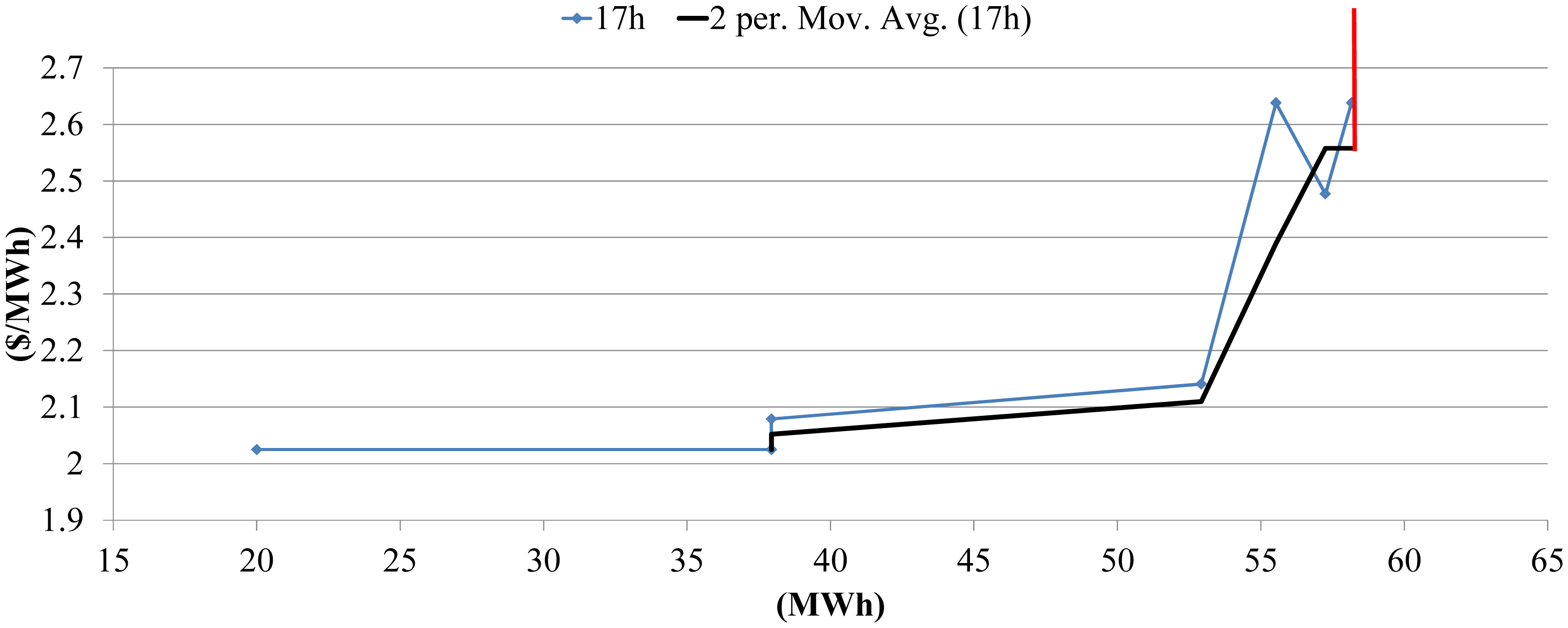
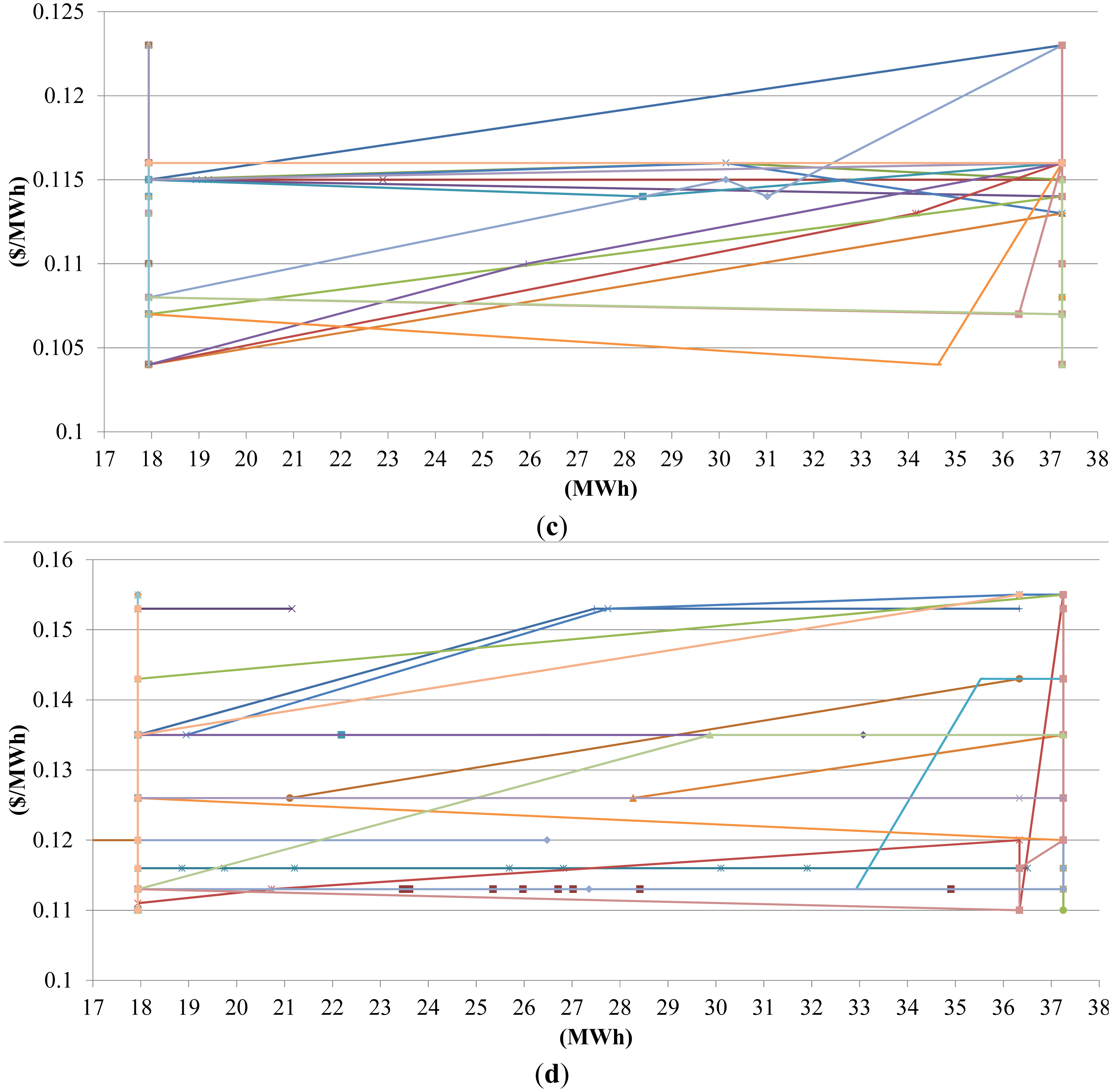
When the function is nonincreasing in some intervals two period moving average approach is used for determining the nondecreasing function as depicted on Figure 11. Also, it is assumed the bid curve is perfectly inelastic in last point as depicted on Figure 11 (red line). Thus, GENCO can create perfectly inelastic bid curve consisting of energy bided marginal cost of producing energy or ancillary (Figure 12).

As the profit tolerance rises from $0 to $1380 for the each hour (Table 3), the profit decreases from $98,193 to $96,959, daily α-VaR increases from $0 to $44,037 and daily α-CVaR increases from $0 to $33120. In other words, when GENCO decides the average hourly profit of 15% worst scenarios should be at least $1380 then GENCO can expect daily profit of $33120 in 15% worst scenarios, the minimal daily profit GENCO can expect with the confidence of 85% is $44,037, and the average profit GENCO can expect is $96,959.

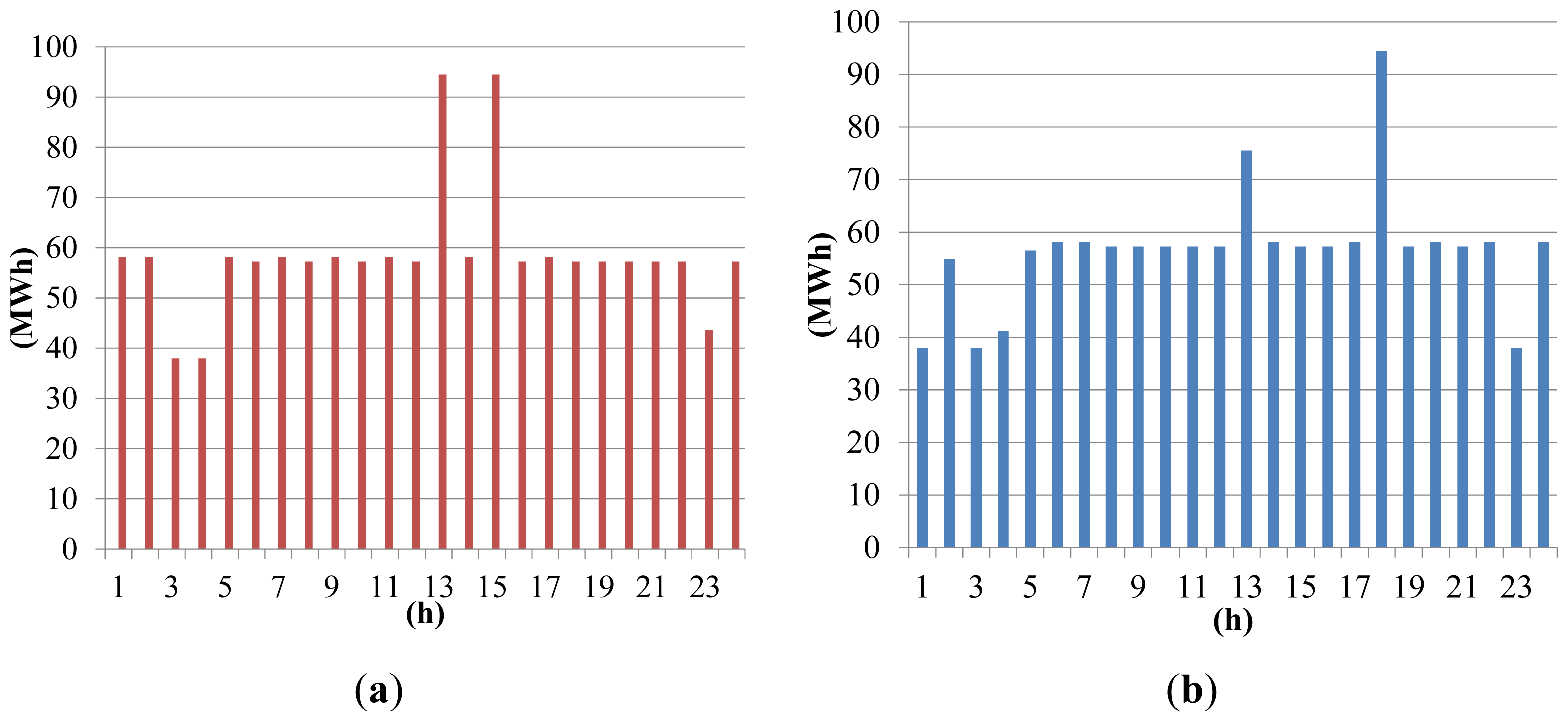
The obtained results confirm a risk aversion principle, generally GENCO should avoid hours with high price deviation as can be seen for the 13-th and 15-th hour in Figure 12. In this case study GENCO should seek certainty even at cost of reducing its profit. The results obtained using normal PDF for representing DAM prices confirm risk aversion principle, but for higher exactness lognormal probability distribution should be used to the pronounce benefits of this approach.

4. Conclusions

The approach presented in this work assesses the problem which the price-taker hydro generating company faces when participating in the simultaneous day-ahead energy and ancillary services markets and which results in the risk-constrained approach for pricing energy and ancillary services.

The results of this case study justify the use of a simplified approach where water shadow price was considered constant over planning horizon. It was also shown that perfectly inelastic bid curves are appropriate for a price-taker hydro generating company. It was shown that reducing risk of financial losses costs, and that these cost can be easily measured.

Since the research was done on relatively small number of scenarios, further work should be done to implement computational efficient algorithms which will tackle dimensionality issue and improve computational time. For higher exactness lognormal probability distribution should be used which will pronounce benefits of this risk-constrained approach.

References

- Zhang, D.; Luh, P.B.; Zhang, Y. A bundle method for hydrothermal scheduling. IEEE Trans. Power Syst. 1999, 14, 1355–1361. [Google Scholar]
- George, A.; Reddy, C.; Sivaramakrishnan, A.Y. Multi-objective, short-term hydro thermal scheduling based on two novel search techniques. Int. J. Eng. Sci. Technol. 2010, 2, 7021–7034. [Google Scholar]
- Dhillon, J.S.; Kothari, D.P. Multi-Objective Short-Term Hydrothermal Scheduling Based on Heuristic Search Technique. Asian J. Inf. Technol. 2007, 6, 447–454. [Google Scholar]
- Zhang, J.L.; Ponnambalam, K. Hydro energy management optimization in a deregulated electricity market. Optim. Eng. 2006, 7, 47–61. [Google Scholar]
- Horsley, A.; Wrobel, A.G. Profit-maximizing operation and valuation of hydroelectric plant: A new solution to the Koopmans problem. J. Econ. Dyn. Control 2007, 31, 938–970. [Google Scholar]
- Perekhodtsev, D.; Lave, L.B. Efficient Bidding for Hydro Power Plants in Markets for Energy and Ancillary Services; 06-003WP; Massachusetts Institute of Technology (MIT) Center for Energy and Environmental Policy Research: Cambridge, MA, USA, 2005. [Google Scholar]
- Koopmans, T.C. Water storage policy in a simplified hydroelectric system. Proceedings of the First International Conference on Operational Reasearch, Oxford, UK, 2–5 September 1957.
- Warford, J.; Munasinghe, M. Electricity Pricing: Theory and Case Studies; The John Hopkins University Press: London, UK, 1982. [Google Scholar]
- Horsley, A.; Wrobel, A.J. Efficiency Rents of Storage Plants in Peak-Load Pricing, I: Pumped Storage; London School of Economics and Political Science: London, UK, 1996. [Google Scholar]
- Horsley, A.; Wrobel, A.J. Efficiency Rents of Storage Plants in Peak-Load Pricing, II: Hydroelectricity; London School of Economics and Political Science: London, UK, 1999; pp. 17–20. [Google Scholar]
- Sorokin, A.; Rebennack, S.; Pardalos, P.; Iliadis, N.A.; Pereira, D. Handbook of Networks in Power Systems; Springer Berlin Heidelberg: Berlin, Germany, 2012; pp. 41–59. [Google Scholar]
- Baillo, A.; Ventosa, M.; Rivier, M.; Ramos, A. Strategic bidding under uncertainty in a competitive electricity market. Proceedings of the International Conference on Probabilistic Methods Applied to Power Systems, Madeira, Portugal, 25–28 September 2000.
- Conejo, A.J.; Nogales, F.J.; Arroyo, M.A. Price-Taker Bidding Strategy under Price Uncertainty. IEEE Trans. Power Syst. 2002, 17, 1081–1088. [Google Scholar]
- Zhang, H.; Gao, F.; Wu, J.; Liu, K.; Liu, X. Optimal Bidding Strategies for Wind Power Producers in the Day-Ahead Electricity Market. Energies 2012, 5, 4804–4823. [Google Scholar]
- Margaris, I.D.; Hansen, A.D.; Sørensen, P.; Hatziargyriou, N.D. Illustration of Modern Wind Turbine Ancillary Services. Energies 2010, 3, 1290–1302. [Google Scholar]
- Lehmann, P.; Creutzig, F.; Ehlers, M.-H.; Friedrichsen, N.; Heuson, C.; Hirth, L.; Pietzcker, R. Carbon Lock-Out: Advancing Renewable Energy Policy in Europe. Energies 2012, 5, 323–354. [Google Scholar]
- Kabouris, J.; Kanellos, F.D. Impacts of Large Scale Wind Penetration on Energy Supply Industry. Energies 2009, 2, 1031–1041. [Google Scholar]
- Garcia-Gonzalez, J.; Parrilla, E.; Mateo, A. Risk-averse profit-based optimal scheduling of a hydro-chain in the day-ahead electricity market. Eur. J. Oper. Res. 2007, 181, 1354–1369. [Google Scholar]
- Garcia-Gonzalez, J.; Parrilla, E.; Mateo, A.; Moraga, R. Building optimal generation bids of a hydro chain in the day-ahead electricity market under price uncertainty. Proceedings of the International Conference on Probabilistic Methods Applied to Power Systems, Stockholm, Sweeden, 11–15 June 2006.
- Rockafellar, R.T.; Uryasev, S. Conditional Value-at-Risk for General Loss Distributions; University of Washington, Department of Mathematics: Seattle, WA, USA, 2001. [Google Scholar]
- Artzner, P.; Delbaen, F.; Eber, J.M.; Heath, D. Thinking coherently. Risk 1997, 10, 68–91. [Google Scholar]
- Acerbi, C. Spectral measures of risk: A coherent representation of subjective risk aversion. J. Bank. Financ. 2002, 26, 1505–1518. [Google Scholar]
- Rockafellar, R.T. Coherent Approaches to Risk in Optimization under Uncertanty. Tutor. Oper. Res. Inf. 2007, 2007, 38–61. [Google Scholar]
- Mariano, S.J.P.; Catalao, J.P.S.; Mendes, V.M.F.; Ferreira, L.A.F.M. Profit-based short-term hydro scheduling considering head-dependent power generation. Proceedings of the IEEE Power Tech 2007, Lausanne, Switzerland, 1–5 July 2007.
- Ponrajah, R.A.; Witherspoon, J.; Galiana, F.D. Systems to optimize conversion efficiencies at Ontario Hydro's hydroelectric plants. Proceedings of the IEEE Transactions on Power Systems, Columbus, OH, USA, 16–19 November 1998.
- Rajšl, I.; Ilak, P.; Delimar, M.; Krajcar, S. Dispatch Method for Independently Owned Hydropower Plants in the Same River Flow. Energies 2012, 5, 3674–3690. [Google Scholar]
- Guo, S.; Chen, J.; Li, Y.; Liu, P.; Li, T. Joint Operation of the Multi-Reservoir System of the Three Gorges and the Qingjiang Cascade Reservoirs. Energies 2011, 4, 1036–1050. [Google Scholar]
- Xu, B.; Zhong, P.-A.; Wan, X.; Zhang, W.; Chen, X. Dynamic Feasible Region Genetic Algorithm for Optimal Operation of a Multi-Reservoir System. Energies 2012, 5, 2894–2910. [Google Scholar]
- Zheng, Y.; Fu, X.; Wei, J. Evaluation of Power Generation Efficiency of Cascade Hydropower Plants: A Case Study. Energies 2013, 6, 1165–1177. [Google Scholar]
- Guan, X.; Svoboda, A.; Li, C.A. Scheduling hydro power systems with restricted operating zones and discharge ramping constraints. IEEE Trans. Power Syst. 1999, 14, 126–131. [Google Scholar]
- Conejo, A.; Arroyo, J.; Contreras, J.; Villamor, F. Self-scheduling of a hydro producer in a pool-based electricity market. IEEE Trans. Power Syst. 2002, 17, 1265–1272. [Google Scholar]
- Nilsson, O.; Sjelvgren, D. Variable splitting applied to modeling of start-up costs in short term hydro generation scheduling. IEEE Trans. Power Syst. 1997, 12, 770–775. [Google Scholar]
- Nilsson, O.; Söder, L.; Sjelvgren, D. Integer modeling of spinning reserve requirements in short term scheduling of hydro systems. IEEE Trans. Power Syst. 1998, 13, 959–964. [Google Scholar]
- The New York Independent System Operator (2012). Available online: http://www.nyiso.com.
- Kuzle, I.; Bosnjak, D.; Tesnjak, S. An Overview of Ancillary Services in an Open Market Enviroment. WSEAS Trans. Power Syst. 2008, 7, 537–546. [Google Scholar]
- Kazempour, S.J.; Hosseinpur, M.; Moghaddam, M.P. Self-Scheduling of a Joint Hydro and Pumped-Storage Plants in Energy, Spinning Reserve and Regulation Markets. Proceedings of the Power & Energy Society General Meeting, Calgary, Canada, 26–30 July 2009.
- Yamin, H.Y. Review on methods of generation scheduling in electric power systems. Sci. Direct. 2003, 69, 153–237. [Google Scholar]
- Ilak, P.; Krajcar, S.; Rajšl, I.; Delimar, M. Profit Maximization of a Hydro Producer in a Day-Ahead Energy Market and Ancillary Service Markets. Proceedings of the IEEE Region 8 Conference EuroCon, Zagreb, Croatia, 2–5 July 2013.
- Hirst, E.; Kirby, B. Creating Competitive Markets for Ancillary Services; U.S. Department of Energy: Oak Ridge, TN, USA, 1997. [Google Scholar]
- Rosenthal, R.E. GAMS/A User's Guide; GAMS Development Corporation: Washington, DC, USA, 2013. [Google Scholar]
- Kuzle, I.; Pandžić, H.; Brezovec, M. Hydro Generating Units Maintenance Scheduling Using Benders Decomposition. Tech. Gaz. 2010, 17, 1–132. [Google Scholar]
- Pandžić, H.; Conejo, A.; Kuzle, I. An EPEC Approach to the Yearly Maintenance Scheduling of Generating Units. IEEE Trans. Power Syst. 2013, 28, 922–930. [Google Scholar]
Nomenclature