Autoregressive with Exogenous Variables and Neural Network Short-Term Load Forecast Models for Residential Low Voltage Distribution Networks

Abstract

This paper set out to identify the significant variables which affect residential low voltage (LV) network demand and develop next day total energy use (NDTEU) and next day peak demand (NDPD) forecast models for each phase. The models were developed using both autoregressive integrated moving average with exogenous variables (ARIMAX) and neural network (NN) techniques. The data used for this research was collected from a LV transformer serving 128 residential customers. It was observed that temperature accounted for half of the residential LV network demand. The inclusion of the double exponential smoothing algorithm, autoregressive terms, relative humidity and day of the week dummy variables increased model accuracy. In terms of R² and for each modelling technique and phase, NDTEU hindcast accuracy ranged from 0.77 to 0.87 and forecast accuracy ranged from 0.74 to 0.84. NDPD hindcast accuracy ranged from 0.68 to 0.74 and forecast accuracy ranged from 0.56 to 0.67. The NDTEU models were more accurate than the NDPD models due to the peak demand time series being more variable in nature. The NN models had slight accuracy gains over the ARIMAX models. A hybrid model was developed which combined the best traits of the ARIMAX and NN techniques, resulting in improved hindcast and forecast fits across the all three phases.

1. Introduction

In recent years there has been substantial interest and speculation in the design and operation of smart grids, micro grids, and distributed energy resources (DER). The reason for this interest is that these emerging technologies may contribute to reducing peak demand and network congestion, minimizing disturbances and increasing network reliability [1–5]. As the technology matures, economic benefits may result from reducing capital and maintenance expenditures and deferring network augmentation [2,5–10].

The sound operation of these emerging technologies will depend on ensuring that supply of power will meet the demand for power [11]. Similar to the conventional electricity generation and supply system, these technologies will rely on accurate forecasting of future electricity demand [5,10–12]. The electricity demand forecasts will need to provide information on how much power is required to be generated at certain times, the scheduling of charging and discharging of energy storage systems, and be able to determine whether or not there are adequate resources to meet future demand with decision points to activate remedial measures such as load shedding, etc.

The current research is part of a larger project to develop an energy management control algorithm to schedule DER in residential low voltage (LV) distribution networks. The DER system incorporates solar photovoltaic (PV) generation and battery energy storage (BES). To adequately schedule DER, information such as the total amount of energy used in a day, magnitude of peak demand can be used to construct demand profiles for future days [13]. Using concepts from Espinoza et al. [14], a pattern recognition based expert system will incorporate forecasts of total energy use and peak demand in order to forecast future demand profiles.

This development total energy use and peak demand forecast models for the residential LV distribution network faces additional challenges due to greater variability and frequency of random “shocks” over modelling subsections of the electricity supply and distribution network which services a greater number of aggregated customers. The greater variability is due to the increase in the influence that individual customers have on the network as the number of customers serviced in a subsection decreases.

This paper sets out to identify the significant variables which influence demand in residential LV distribution networks and develop next day total energy use (NDTEU) and next day peak demand (NDPD) forecast models for each phase of a residential LV distribution transformer servicing 128 customers. Autoregressive integrated moving average with exogenous variables (ARIMAX) and neural network (NN) modelling techniques will be used to construct the NDTEU and NDPD models in order to draw model accuracy comparisons and determine whether or not combining the techniques will yield more accurate models.

2. Research Background

Griffith University, Elevare, Ergon Energy and Energex, under the Queensland State Government 2012–2014 Research Partnership Grant, are participating in a large joint project to research and determine the feasibility of installing static synchronous compensators (STATCOMs) with BESS in the LV distribution network in the South East Queensland (SEQ) region of Australia. STATCOMs are four quadrant pure sine wave synchronous inverters. STATCOMs are able to import and export real and reactive power, correct frequency distortions and dampen harmonics. Integrating STATCOMs with DER has the potential to mitigate DER power quality issues as noted by Ackermann and Knyazkin [1], Enslin and Heskes [15]. STATCOMs with BES have the ability to reduce peak demand through load shifting and also contribute to the enhanced management of power quality. Reducing peak demand and maintaining power quality have the potential to reduce network operational expenditures through the deferral of greater capital expenditures such replacing transformers and/or upgrading lines. The ultimate goal of the joint project is to design and quantify the effectiveness of STATCOMs with BES for reducing network infrastructure expenditures over their life cycle. The widespread implementation of STATCOMs with BES in the LV distribution network will be considered to be feasible if they have a life cycle cost that is lower than the business as usual scenario for providing power in the region.

3. Literature Review

3.1. Short-Term Electricity Demand Forecasting

The length of the scheduling window for the energy management control algorithm is determined by the capacity of the BES and the level of the network in which the BES will be installed (e.g., customer, LV distribution network, and high voltage distribution network). Larger BES will be able to reliably achieve their objectives over time under conditions of charging and discharging. For the current research the capacity of the BES is limited by the cost of lithium-ion batteries. This financial constraint curtails the scheduling window of the energy management control algorithm. In conjunction with BES in the LV distribution network, the length of the scheduling window is limited to three days into the future. Regardless of battery costs, readers should note that there is a rapidly diminishing return from the long-term storage of power for the purpose of levelling spikes in demand in an LV network.

The length of the scheduling window bounds the daily peak demand and total electricity demand forecast models to the short-term forecasting horizon. Short-term forecast models focus on forecasting time intervals of minutes, hours, days to a week into the future. The most common techniques used to construct short-term forecast models include multivariable regression, time series analysis techniques and machine learning algorithms such as NNs [16–23]. These techniques have been successfully applied to national grid level demand time series [16–23]. It has been observed that there is a limited amount of published literature on LV distribution network applications.

3.2. Summary of Modelling Techniques

Multivariable regression models are based on the use of the least mean square algorithm to estimate the coefficients of the model parameters. Model parameters are selected by the modeller with the aid of exploratory statistics to infer whether or not there are relationships between independent variables and the dependent variable the model is attempting to explain. Periodicities observed in the dependent variable can be identified by the use of the Discrete Fourier Transform and inserted into the model as a basis function. Diagnostic tests such as the f-test and t-test on regression coefficients reveal whether or not model parameters are statistically significant at a particular threshold level of significance (α). The calculation of the coefficient of determination (R²) and root mean square error (RMSE) describe the accuracy of the model in explaining the dependent variable.

Time series techniques, codified by Box and Jenkins [24], are a set of modelling techniques which involve constructing forecast models with parameters based on permutations of the variable the model is to forecast. The autoregressive integrated moving average (ARIMA) p, d, q, is the general model of the time series techniques which encapsulates the autoregressive model, non-seasonal differencing and the moving average model. The “p” term represents the number of time lagged parameters; the “d” term represents the number of discrete differences the forecast variable's data has undergone in order to remove seasonality; and the “q” term represents the number of time lagged forecast error parameters in the model to account for an observed moving average in the forecast variable's data. The order of “p” and “q” terms can be identified by the use of the partial autocorrelation function. The level of difference can be determined by the use of an autocorrelation plot based on the nature of decay or the use of the Durbin-Watson (DW) statistic to identify autocorrelation in the forecast error (serial correlation). Coefficients of time series models can be estimated by regression or maximum likelihood estimators.

NNs are a set of modelling techniques which have a wide range of applications including statistical modelling, discrete classification, pattern recognition, control systems, etc. NNs mimic how biological NNs operate and learn. NNs are constructed from multiple layers of neurons connected by weights from each neuron to each neuron of the proceeding layer. Neurons are the base unit of the network. The weights between the neurons represent a linear augmentation of the outputs from the previous layer's neurons. Individual neurons summate the previous layer's outputs multiplied by the weights and the result is processed in an activation function. Through a specified learning algorithm, the training process alters the weights throughout the network until the network has been identified to be an optimal model which explains the dependent variable. The main benefit of using the NN methodology over other techniques is that it is able to identify non-linear relationships between the independent and dependent variables.

3.3. Representative Publications

Engle et al. [16] set out to identify a next day peak electricity demand forecast model by testing univariate, bivariate and weather variable models. The coefficients of the models were estimated using regression. Engle et al. [16] used Consumer Power's peak demand data for 1983 and 1984 for training and validation of the models. The highest performing univariate model was constructed with an autoregressive variable and holiday, holiday for the previous day, Saturday, Sunday and Monday dummy variables. The bivariate model consists of two stages. Stage one consists of a forecast of the next day's average electricity demand. Stage two uses the forecast of the average electricity demand as an input variable in the NDPD forecast model. Additional variables in the model were the same as the univariate model with an additional average electricity demand of the previous demand variable. The weather variable model was first constructed using the same variables as the univariate model with an additional lag of average demand variable. Weather variables included in the model were heating and cooling day variables which are determined by temperature thresholds. Engle et al. [16] concluded by stating that the weather variable model was the best performing due to having the best validation statistics out of the set of models examined.

In an investigation of whether or not NNs are a better modelling technique than ARIMA, Darbellay and Slama [17] constructed short-term (hourly) electricity demand models from the Czech Republic's 1994 and 1995 electricity demand data for comparison purposes. The Czech Republic's electricity demand data exhibited daily, weekly and yearly cycles. The first stage in the investigation was to determine whether or not there were non-linear autocorrelations by use of the mutual information criterion and to identify significant variables (representative seasons in the data). A univariate model and a model with an additional weather variable were constructed and compared using the two examined modelling techniques. The results suggested that the autocorrelations of the electricity demand data were predominantly linear which highlights that linear modelling techniques are suitable. The ARIMA and NN univariate models performed similarly while the ARIMA model with additional weather variables performed better than the NN.

Ringwood et al. [18] used NN modelling techniques to develop short, medium and long-term electricity forecast models and compared the models against conventional techniques such as Box-Jenkins time series models. The structure of the models was determined by the use of the autocorrelation function. The comparison of the models displayed that the NN model performed better than the Box-Jenkins time series model.

In univariate models the seasonality as identified by the use of the autocorrelation and partial autocorrelation algorithms are the key determinants in forecasting future demand. If the time series is non-stationary, the change in mean must be accounted for. The Holt-Winters Seasonal Exponential Smoothing algorithm takes into account the local trend, moving average and the seasonality in the time series to produce a forecast model. Taylor [19] set out to improve online univariate models by adapting the Holt-Winters Seasonal Exponential Smoothing algorithm to take into account an additional seasonal influence (Double Seasonal Exponential Smoothing). Taylor [19] used half-hourly electricity demand data from England and Wales and compared the Holts-Winters Seasonal Exponential Smoothing and double exponential smoothing (DES) with daily and weekly seasonality. Once controlling for autocorrelation in the error term, Taylor [19] noted that the DES model performed better. Taylor [20] went on to adapt the algorithm to take into account three seasons and found that the method improved forecast accuracy.

Taylor and Buizza [21] noted that weather variables are important determinants in short to medium electricity demand forecast models. To improve on current methods of forecasting electricity demand based on weather variables, Taylor and Buizza [21] used forecasted weather ensembles to forecast multiple scenarios of future electricity demand. Ensemble forecasting is a method whereby a set of future states of a dynamic system is forecasted based on slightly different initial conditions. This technique is typically used in weather forecasting. Taylor and Buizza [21] based the electricity demand forecast model off England's National Grid's weather dependent forecast model. The forecast model involves effective temperature, cooling power of wind and effective illumination. The weather ensembles were inputted into the model and the mean of the results were used as the forecast. The weather ensemble method was compared against a traditional weather model, actual weather for forecasting and an ARMA model with Friday, Saturday and Sunday dummy variables. Taylor and Buizza [21] found that the weather ensemble method performed better than the traditional weather and ARMA models.

Mirasgedis et al. [22] developed a daily and monthly electricity demand forecast models using weather variables. The non-linear response between temperature and electricity demand was decomposed into heating and cooling variables. The daily electricity demand forecast model was composed of heating and cooling variables and lags of the variables, humidity variables, day of the week dummy variables, month of the year dummy variables, holiday dummy variable and autoregressive variables to correct for autocorrelation of the error term. The coefficients of the model were estimated by regression.

Support vector regression (SVR), dual extended Kalman filter (DEKF) and a radial basis function NN (RBFNN) were combined by Ko and Lee [23] to create a short-term load forecast model with data from the Taipower Company (Taipei, Taiwan). The technique was then compared against a DEKF-RBFNN model and a RBFNN model. The SVR and the DEKF are used to determine the optimal inputs for the RBFNN from independent variables. Ko and Lee [23] found that the combination of SVR, DEKF and RBFNN created a short-term forecast model which outperformed other models.

Hernández et al. [13] developed a next day demand profile forecast system for a micro grid by the use of a two stage system. The first stage is comprised by a series of NNs which forecasts demand profile properties such as peak loads and valley loads. The forecasts are fed into the second stage's NN which produces a demand profile forecast with 24 values for each hour of the day. Demand data from Castilla y León (Spain) was used to train and validate the NNs. The system forecasted demand profiles with a high level of accuracy and boasted improvement in forecast accuracy over previous work.

3.4. Model Selection

The significant variables which dictate the parameters of electricity demand forecast models are determined by the scope of the forecast models. Weather variables have little effect on short-term forecast models which forecast half-hourly or hourly ahead of time and are generally not used [19]. The results of Darbellay and Slama [17] displayed that the models without temperature variables performed insignificantly better.

As the forecast window is increased to forecasting a day ahead and greater, weather variables become more significant. In the next day load forecast models developed by Engle et al. [16], Taylor and Buizza [21], Mirasgedis et al. [22], weather variables were significant components. Engle et al. [16], Taylor and Buizza [21] found that models with weather variables performed better than the comparison time series models.

Electricity demand time series data is non-stationary and contains many seasonal trends [17–21]. The seasonalities in the data are identified by the use of the autocorrelation and partial autocorrelation algorithms. Darbellay and Slama [17] and Taylor [19] identified daily, weekly and annual trends which were used as variables in their models. The daily electricity demand forecast models developed by Mirasgedis et al. [22] included day of the week and month of the year dummy variables. These dummy variables account for weekly and annual seasonality in the data set.

The proposed NDTEU and NDPD forecast models will require weather and seasonality variables to be effectively incorporated and the non-stationarity characteristics of electricity demand time series to be mitigated. The selected modelling techniques to develop the NDTEU and NDPD forecast models are ARIMAX and feed forward back propagation NN. ARIMAX is the general ARIMA model with the inclusion of exogenous variables such as weather variables. The NN models will have a similar input variable structure including both autoregressive terms and exogenous variables.

The results of the ARIMAX and NN models will be compared to determine which technique is most suitable.

4. Data

4.1. Source

Data for the LV transformer used in the construction of the load forecast models has been collected and provided by Energex (i.e., the power distribution company for the SEQ region). The transformer is located in an inner northern suburb of Brisbane, Queensland. The transformer distributes power to 128 residential customers. The metering resolution was such that the voltage, current and line to neutral power factor for each phase of the transformer was recorded at 10 min intervals. The data set covers the period from the middle of January 2012 to mid-February 2013. Weather data such as temperature and relative humidity (RH) were collected by the Brisbane City weather station, made publically available by the Australian Bureau of Meteorology and downloaded from their website. The first half of the data set was used for coefficient estimation or NN training and the second half of the data set was used for model validation.

The Brisbane resides in a subtropical climate region which is denoted by mild winters and hot humid summers. According to the Australian Bureau of Meteorology [25], January is the hottest month of the year with average maximum and minimum temperatures of 29.0 °C and 21.2 °C. July is the coldest month of the year with average maximum and minimum temperatures of 20.8 °C and 9.0 °C. The annual precipitation is 1028.2 mm where the greater majority of precipitation occurring during the months from November to March.

4.2. Overview

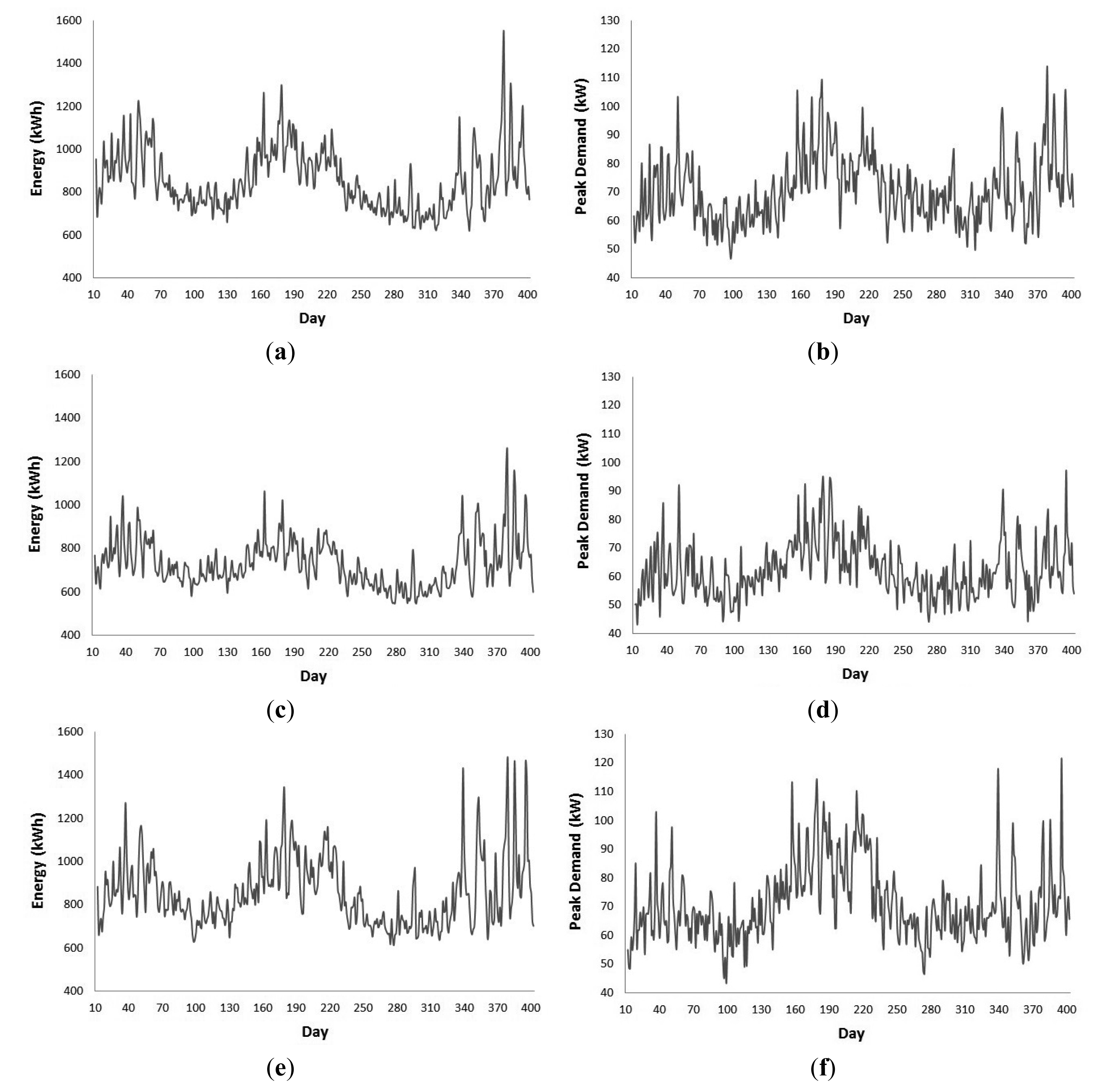
Figure 1 illustrates the daily total energy use and daily peak demand for each phase of the transformer. The period displayed by the graphs starts from the 12 January 2012 (Day 12) to the 6 February 2013 (Day 403). The daily peak demand data for each phase have greater variability than the daily total electricity demand. The system is unbalanced with Phase 3 incurring the greatest load. The transformer experiences greater loads with higher variance during the summer and winter periods of the year. The yearly peak demand on the transformer occurs during summer. From these observations it can be stated that the daily total energy use and daily peak demand time series are non-stationary.

The transformer incurred an abnormally high load on the 11 June 2013 (Day 12), which was the Queen's Diamond Jubilee public holiday. Other public holidays did not coincide with loads abnormal for their respected times of the year. The suburb where the data was collected resides within an area with a high risk of flooding. As a result, the demand in the system is significantly higher the day after a period of heavy rainfall in the greater catchment area when controlling for other variables. The most notable spike in demand occurred on the 29 January 2013 (Day 395) in response to heavy rainfall and flooding which occurred during the preceding days. These events are considered to be exogenous shocks to the system and can't be forecasted ahead of time. To avoid biasing the models' accuracy statistics, the exogenous shock data points were not removed.

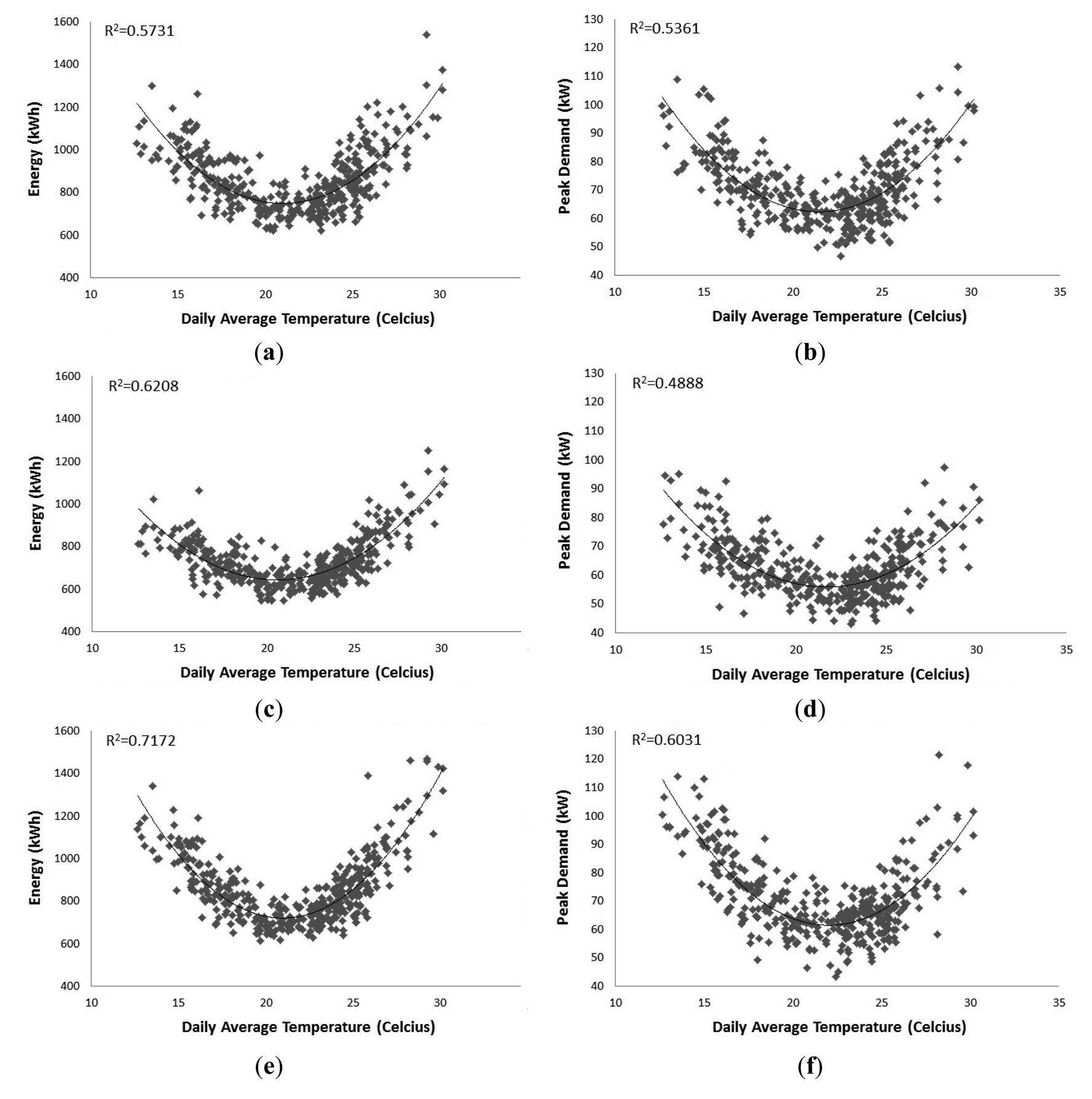
Figure 2 displays the daily total energy use and daily peak demand temperature response for each phase of the transformer. What can be noted from each of the graphs is that the demand response to temperature is parabolic in nature. Greater loads are experienced during days with average temperatures below 18 °C and above 26 °C. This reinforces the observation from Figure 1 that during winter and summer months the transformer experiences greater loads. Daily average temperature explains daily total electricity demand with R² ranging from 0.57 to 0.71. In comparison, daily average temperature explains daily peak demand to a lesser degree with R² ranging from 0.48 to 0.60. Daily average temperature as a single determinant explains half or greater of the observed variance. This suggests that daily average temperature would be a key determinant in forecasting daily total energy use and daily peak demand. The temperature response observation is in line with weather variable observations made by Engle et al. [16], Taylor and Buizza [21] and Mirasgedis et al. [22].

5. Research Method

5.1. Overview

The following main steps outline the method for constructing the three clusters of forecast models (i.e., ARIMAX, NN and hybrid ARIMAX-NN):

(1)

Establish the modelling framework;

(2)

Forecast day-ahead local mean using the double exponential smoothing (DES) algorithm;

(3)

Selection of autoregressive terms;

(4)

Selection of exogenous variables;

(5)

Coefficient estimation; and

(6)

Validation of models.

A confidence interval of 95% was used for the calculation of critical values.

5.2. ARIMAX Model

The selected modelling approach to construct the NDTEU and NDPD forecast models was the ARIMAX model. As previously noted, the ARIMAX model combines the ARIMA model with exogenous variables. To fulfil the ARIMA model component of the ARIMAX model, the Holt-Winters DES algorithm was employed as a model input variable. DES is analogous to an ARIMA (0, 2, 2) model which accounts for a changing mean throughout the time series and low frequency seasonality. The general ARIMAX model is described by Equation (1):

$$y_t=\mathrm{\rho }{F}_t+\sum _{i=1}^p{\mathrm{\beta }}_i{y}_{t-i}+\sum _{j=1}^r{\mathrm{\omega }}_j{w}_j+e_t$$

(1)

where y_t is the demand at time t; F_t is the forecasted mean for time t calculated by the DES algorithm; ρ is the model coefficient for F_t; y_t−i is the demand lagged by i time steps; β_i is the coefficient of y_t−i; p is the maximum number of time lags; w_j represents the model's exogenous variables; ω_j represents the coefficients of the exogenous variables; r is the maximum number of exogenous variables; and e_t is the error at time t. The coefficients of the models are estimated by regression.

5.3. NN

The feed forward error back propagation NN was used. The output of each neuron throughout the network is calculated by Equations (2) and (3):

$$v_i=\sum _{h=1}^m{w}_{ih}{x}_h$$

(2)

where v_i is the summation of the weights w connecting to the inputs x for neuron i. There are m inputs with corresponding weights in the previous layer h. If layer h is a hidden layer, each x_h is an output of a neuron from the previous layer.

$${Ŷ}_i=\sigma (v_i)=\frac{1}{1+exp(-v_{i}a)}$$

(3)

where Ŷ_i is the output of neuron i; σ(v_i) is the sigmoid activation function and a is a constant which influences the gradient of the function.

The training of weights throughout the network is calculated using two algorithms. The first algorithm, Equations (4) and (5), apply to the weights connecting to the last layer of neurons in the network. The second algorithm, Equations (6) and (7), apply to the weights connecting to neurons within hidden layers:

$${\delta }_j={\sigma }^{\prime }(v_j)({Ŷ}_{j-}{Y}_j)$$

(4)

$$w_{ji}^{(t+1)}=w_{ji}^{(t)}+\mathrm{\tau }{\mathrm{\delta }}_j{Y}_i$$

(5)

where δ_j is the local gradient at neuron j; Ŷ_j is the forecast; Y_j is the observed value; Y_i is the output from neuron i of the previous layer; w_ji is the weight connecting neuron i to neuron j; τ is the training rate; and t is the training iteration:

$${\mathrm{\delta }}_i={\sigma }^{\prime }(v_i)\sum _{j=1}^k{\mathrm{\delta }}_j{w}_{ji}$$

(6)

$$w_{ih}^{(t+1)}=w_{ih}^{(t)}+\mathrm{\tau }{\mathrm{\delta }}_i{Y}_h$$

(7)

where δ_i is the local gradient at neuron I; k is the number of neurons in the proceeding layer; w_ih is the weight connecting neuron i to neuron h of the previous layer; and Y_h is the output of neuron h.

20% of the training data set is randomly separated to form a calibration set which is not used for updating the weights to ensure that the network does not over-fit the data. The training process is constrained by a maximum number of training iterations defined by the user. Accuracy statistics for the training and calibration sets are calculated for each iteration and if the accuracy statistics for both sets improve, the weights throughout the network are saved. The process continues until the maximum number of iterations is reached.

5.4. DES

The DES algorithm is referenced from Gardner and Dannenbring [26] and is outlined by Equations (8)–(10):

$$s_t=\mathrm{\gamma }{y}_t+(1-\mathrm{\gamma })(S_{t-1}+b_{t-1})$$

(8)

$$b_t=\mathrm{\theta }(s_t-s_{t-1})+(1-\mathrm{\theta })b_{t-1}$$

(9)

$$F_{t+1}=s_t+b_t$$

(10)

where s_t is an estimate of the mean at time t; b_t is an estimate of the slope at time t; y_t is the demand at time t; F_t is the forecast of the mean at time t; γ and θ are smoothing constants estimated by an optimisation algorithm.

5.5. Autoregressive Terms

The autoregressive terms of the models were selected from the use of the partial autocorrelation function and the DW statistic. Once the partial autocorrelation function has been calculated, lags with partial correlations above the threshold level (calculated by Equation (11)) are then identified as being significant. The DW statistic identifies whether or not the model's error term is autocorrelated. The addition or subtraction of autoregressive terms can mitigate positive or negative autocorrelation. If the addition or subtraction of autoregressive terms does not mitigate the autocorrelation in the error, a process of differencing is required to be undertaken. The DW statistic is calculated by Equation (12):

$$\pm \frac{Z_1-(\mathrm{\alpha }/2)}{n^{1/2}}$$

(11)

where z is a two-tailed score from Student's t-distribution with a level of significance α/2; and n is the number of observations in the time steps within the time series. For the current research a confidence interval of 95% is assumed, therefore, α equals 0.05:

$$DW=\frac{{\sum }_{t=2}^n{\left(e_t-e_{t-1}\right)}^2}{{\sum }_{t=2}^n{\left(e_t\right)}^2}$$

(12)

where DW is the DW statistic, e_t is the model residual at time t; and n is the number of observations in the time series. The DW statistic is compared against positive and negative autocorrelation thresholds at a level of significance α.

5.6. Exogenous Variables Selection and Validation

The selection of exogenous variables was conducted based on a priori analysis to discern the response and a stepwise regression approach. Individual variables are added to each model and the accuracy statistics are calculated based on the coefficient estimation set or training and calibration sets. If the inclusion of a variable increases model accuracy, the variables is used. The accuracy of each model is estimated by forecasting over the validation time period and comparing the results against observations.

6. Results

6.1. ARIMAX Models

6.1.1. Coefficient Estimation and Hindcast Accuracy

Table 1. ARIMAX coefficient estimates. NDTEU: next day total energy use; NDPD: next day peak demand; RH: relative humidity; and DES: double exponential smoothing.

Variables	NDTEU (kW·h) Coefficients			NDPD (W) Coefficients
	Phase			Phase
	1	2	3	1	2	3
Intercept	-	-	-	137,073.52	133,737.77	202,479.53
Demand t-1	0.35	0.36	0.36	0.10	0.14	0.16
Demand t-2	−0.15	−0.09	−0.18	−0.12	−0.01	0.03
Temp.	−129.82	−87.79	−211.13	−11,655.72	−11,419.61	−17,935.12
Temp.2	3.47	2.41	5.35	288.67	279.51	429.94
RH	17.70	12.80	14.83	1,391.22	798.41	1,014.73
RH × Temp.	−1.38	−1.00	−1.13	−119.84	−62.29	−74.69
RH × Temp.2	0.03	0.02	0.02	2.49714	1.168	1.33
WDSun	1,577.84	1,201.33	2,556.78	23,764.67	24,592.98	31,945.33
WDSat	1,554.45	1,167.41	2,548.66	18,074.01	16,891.21	26,996.29
WDMon	1,509.32	1,139.58	2,530.62	22,391.29	20,958.81	32,323.91
WDTues	1,517.58	1,130.39	2,526.15	20,441.31	19,444.24	30,004.19
WDWed	1,508.34	1,139.25	2,536.47	19,077.26	20,602.11	29,372.48
WDThurs	1,515.09	1,120.43	2,515.01	19,064.74	17,876.66	27,327.90
WDFri	1,487.91	1,112.31	2,506.79	14,260.18	13,371.69	24,509.34
DES forecast	0.29	0.13	0.14	0.39	0.20	0.04

displays the results of the variable selection process and the value of each variable's coefficient. The partial autocorrelation function displayed that there were either one or two significant autoregressive terms for each model. The DW test applied to initial model constructions displayed that the error term was positively autocorrelated for models which had one autoregressive term. An additional autoregressive term was added to these models to remove the autocorrelation in the error term. The observed parabolic temperature response, revealed in Figure 2, was added to the models in the form of Temp. and Temp.² variables. RH and RH interacting with the parabolic demand response to temperature (i.e., RH × Temp. and RH × Temp.² variables) was added to the models which increased hindcast accuracy statistics. The day of the week dummy variables were added to account for the effects that different days of the week have on demand. As previously discussed, the DES forecast accounts for the changing mean throughout the year. The NDPD models differed from the NDTEU models due to the inclusion of an intercept.

The results of the DW tests suggest that there is no autocorrelation in the models' error terms. It can be inferred that the absence of autocorrelation in the error terms means that the RMSE and R² statistics are unlikely to be biased. The results of the f-test on regression coefficients are of higher magnitude than the level of significance suggesting that the set of coefficients are not statistically equivalent to zero. The t-test on regression coefficients displays that many coefficients are not statistically significant. During stepwise regression processes, when these variables were removed the RMSE increased and R² decreased. This coincided with the removal of the effects that different weekdays had on demand and the promotion of a temperature response which is not represented in the data. In order to achieve models with the best fits, these variables were not removed. This phenomenon can be attributed to the greater magnitudes of the Temp.², DES mean forecast and demand lag variables in comparison to temperature and day of the week dummy variables.

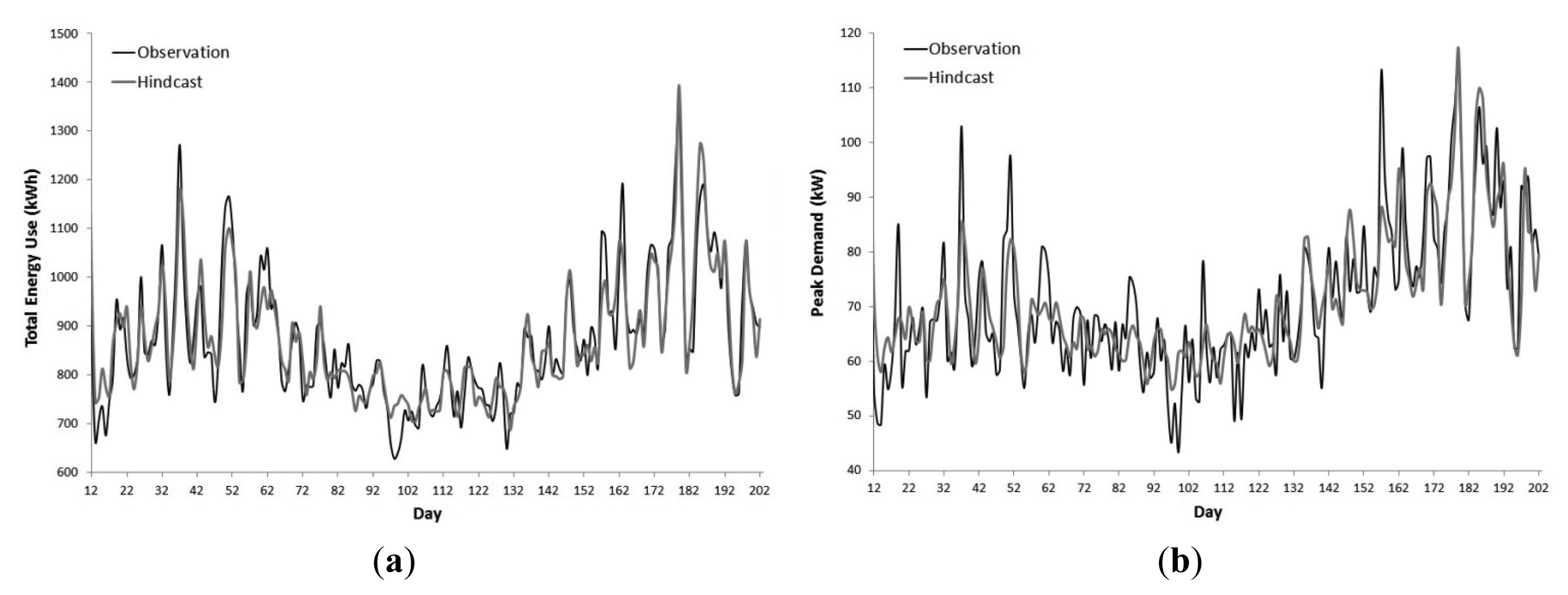
Figure 3 displays Phase 3's ARIMAX NDTEU and NDPD hindcasts which are representative of the other two phases. The greater majority of both hindcasts align well with the observed data. Divergences between the NDTEU hindcasts and observed data were observed on Days 157 and 163. The divergence on Day 157 may be attributed to a spike in demand in response to a period of rainfall and a low daily temperature. Day 163 was a unique public holiday relating to the Queen's Diamond Jubilee, which had an abnormal spike in demand. In addition to Day 157, the NDPD hindcasts deviate from observations on Days 19, 32, 37, 51, 60, 81 and 106. The divergences on Days 19, 32, 37, 51, 60 and 81 coincide with high maximum daily temperatures above 30 °C.

Table 2. ARIMAX hindcast statistics. RMSE: root mean square error; MAPE: mean absolute percentage error; and DW: Durbin-Watson.

Variables		NDTEU (kW·h)			NDPD (W)
		Phase			Phase
		1	2	3	1	2	3
RMSE		55.60	46.11	55.31	6,814.87	6,038.91	7,447.68
R2		0.84	0.77	0.87	0.72	0.70	0.72
MAPE (%)		4.51	4.21	4.44	7.05	7.12	7.81
DW	Dl		1.63			1.63
	Du		1.90			1.90
	Stat.	1.80	1.85	1.73	1.8	1.91	1.81
f-test	Sig.		1.7			1.7
	Stat.	71.03	45.09	87.96	30.98	27.50	32.14
t-test, Sig.			1.96			1.96
Intercept		-	-	-	0.00	0.00	1.70
Demand t-1		101.74	90.56	139.03	17.47	25.64	33.21
Demand t-2		45.63	24.62	80.29	24.56	2.15	7.43
Temp.		0.08	0.08	0.15	0.00	0.00	0.00
Temp.2		3.84	3.89	6.65	0.02	0.03	0.03
RH		0.41	0.43	0.39	0.00	0.00	0.00
RH × Temp.		3.34	3.51	3.09	0.02	0.01	0.01
RH × Temp.2		115.57	119.92	103.29	0.70	0.43	0.32

presents the ARIMAX hindcast accuracy statistics. The NDTEU models performed better than the NDPD models with R² statistics ranging from 0.77 to 0.87. The NDPD models had R² statistics ranging from 0.70 to 0.72. The lower accuracy of the NDPD models in comparison to the NDTEU models can be attributed to the peak demand time series having greater variance than the total energy use time series.

6.1.2. Validation Accuracy

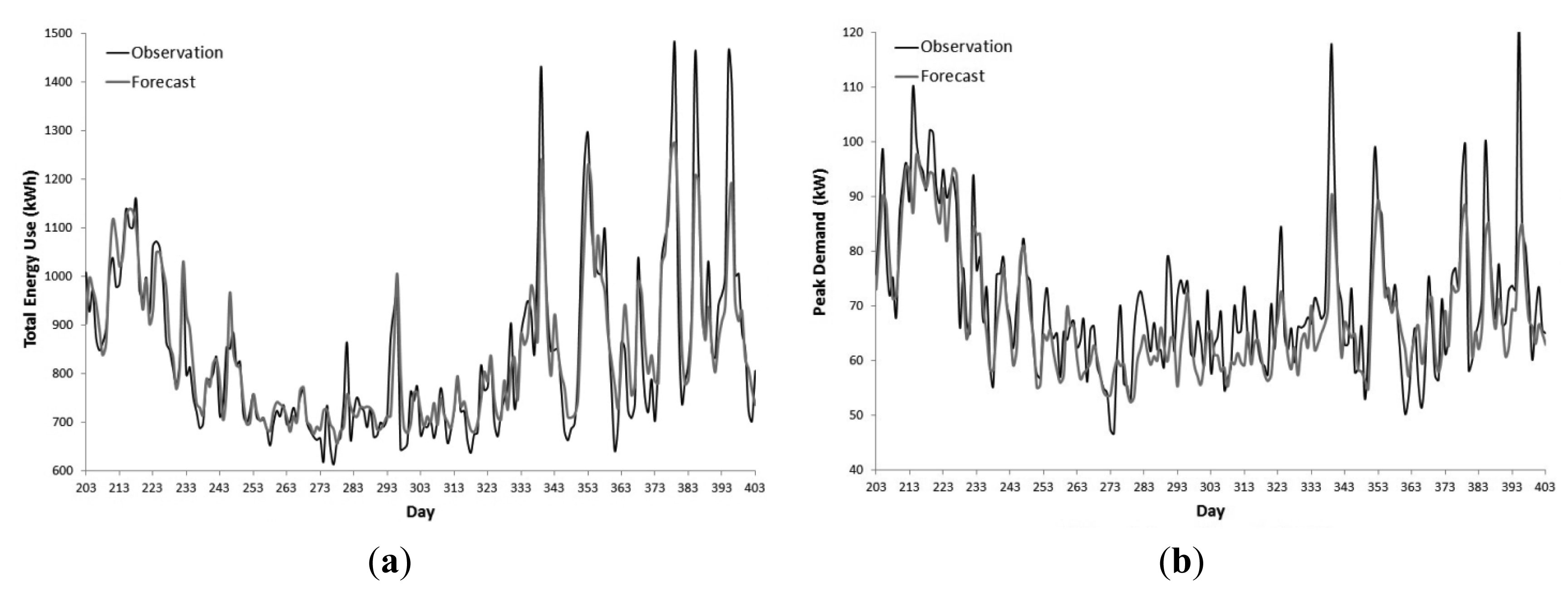
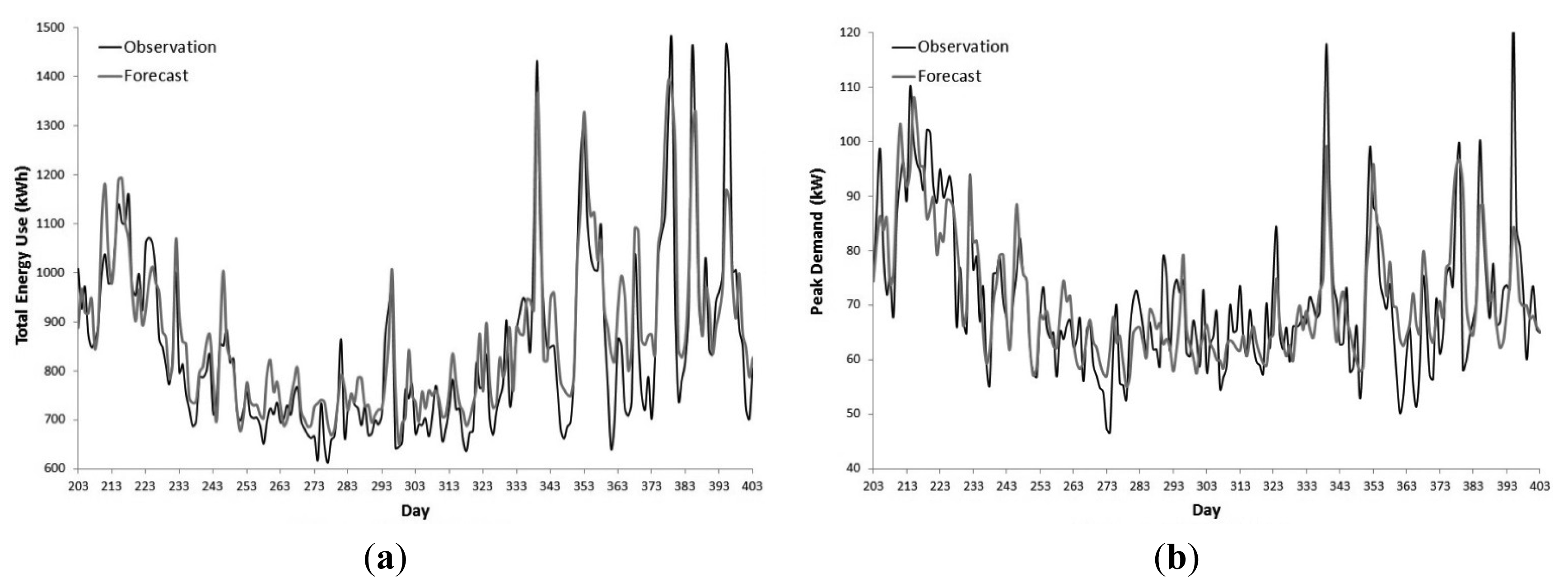
Figure 4 illustrates Phase 3's ARIMAX NDTEU and NDPD forecasts against the validation set. From Day 203 to Day 393 the forecasts mostly followed the observed data. Following the trend of the hindcasts, the NDPD models exhibit a curtailed ability to forecast large demand spikes coinciding with daily maximum temperatures above 34 °C as seen on Days 339, 385 and 395. The NDTEU models were better able to forecast demand on Days 339 and 385. On the 29 January 2013 (Day 395), the high spike in demand occurred on the day after a period of heavy rainfall and flooding. This exogenous shock resulted in a discrepancy between the forecast and observed data in this period.

Table 3. ARIMAX validation statistics.

Accuracy Statistics	NDTEU (kW·h)			NDPD (W)
	Phase			Phase
	1	2	3	1	2	3
RMSE	75.71	58.21	83.92	7,516.50	6,336.00	8,070.56
R2	0.74	0.80	0.78	0.58	0.56	0.65
MAPE (%)	6.97	6.30	7.33	7.90	7.48	8.13

displays the accuracy statistics of the ARIMAX models' forecasts against the validation set. The NDTEU forecasts had a better fit to observed data than the NDPD forecasts. In comparison to the hindcasts, the forecasts had poorer fits with R² statistics ranging from 0.74 to 0.80 for the NDTEU models and from 0.56 to 0.65 for the NDPD models. NDTEU R² statistics decreased on the order of from 0.03 to 0.1 and MAPE increased by 2% to 2.9%. NDPD R² statistics decreased by 0.07 to 0.14 and MAPE increased by 0.36% to 0.75%.

6.2. NN Models

6.2.1. Training and Hindcast Accuracy

The NN models had similar variables to the ARIMAX models. The NDTEU NN models included one autogressive term (i.e., Demand t-1), parabolic demand response to temperature, RH, RH-temperature interaction, day of the week dummy variables and DES forecast variables. The NDPD NN models included two autoregressive terms (i.e., Demand t-1 and Demand t-2), parabolic demand response to temperature, RH, RH-temperature interaction, day of the week dummy variables and DES forecast variables. The NDTEU models differed by the NN models including one autoregressive term rather than two. The NDPD models differed by the NN models not including an intercept variable. All NN models had one hidden layer with the number of neurons in that layer ranging from 25 to 40.

NN have the ability to emulate non-linear relationships between the input variables and observations. During the process of constructing and training the NN models, it was observed that denoting the parabolic response that demand had to temperature (i.e., Temp. and Temp.² variables), the training and calibration accuracy statistics improved and the models were better able to account for the response. This formed the argument for the inclusion of additional variables rather than a singular variable to account for the non-linear relationships.

Table 4. NN hindcast statistics.

Accuracy Statistics		NDTEU (kW·h)			NDPD (W)
		Phase			Phase
		1	2	3	1	2	3
RMSE		57.74	38.30	55.72	6,656.64	6,192.00	7,187.67
R2		0.83	0.84	0.85	0.73	0.68	0.74
MAPE (%)		4.82	3.87	4.53	6.85	7.36	7.41
DW	Dl		1.63			1.63
	Du		1.90			1.90
	Stat.	1.92	1.86	1.78	1.81	2.04	2.09

contains the NN hindcast accuracy statistics. Similar to the ARIMAX models, the NDTEU models performed better than the NDPD models with R² statistics ranging from 0.83 to 0.85. The NDPD models had R² statics which were 0.10 to 0.16 less than the NDTEU models. The DW statistics across the models indicate there is no positive or negative autocorrelation in the error terms. The NN models exhibited a similar level of hindcast accuracy as the ARIMAX models.

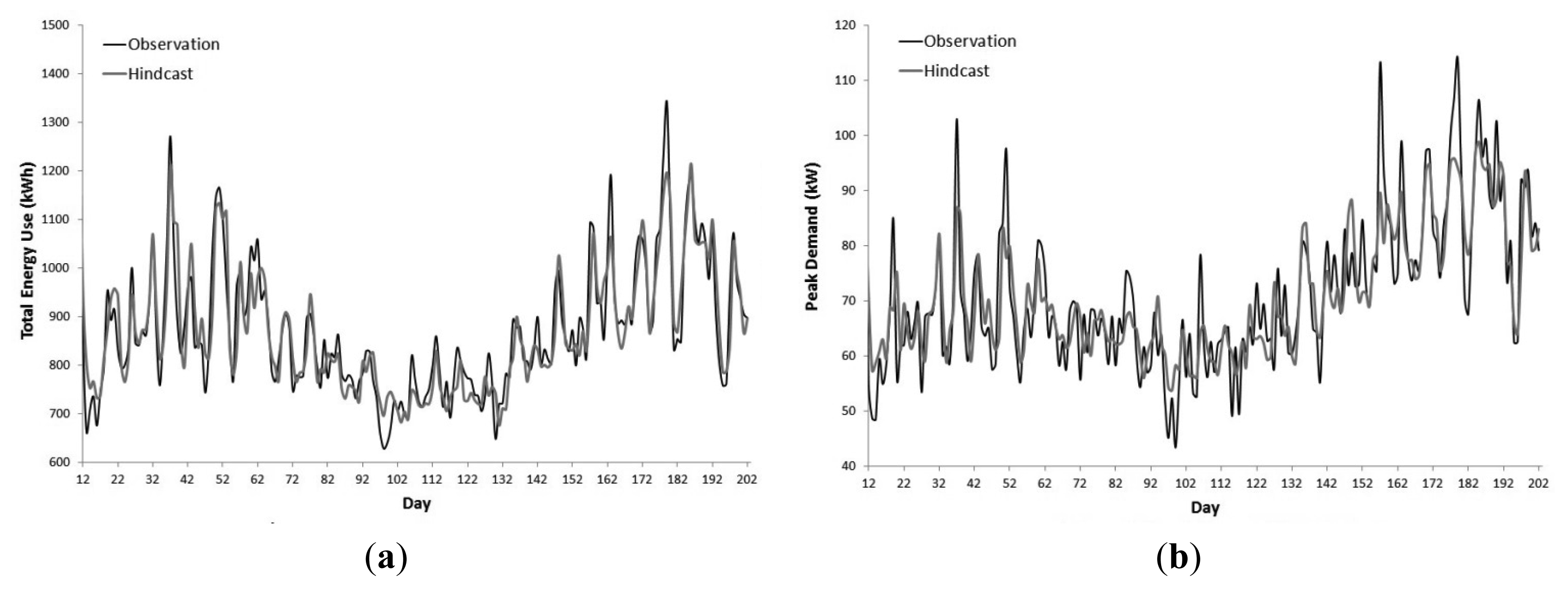
Figure 5 displays Phase 3's NN NDTEU and NDPD hindcasts. The NN hindcasts fit the observations in the training set well for the majority of the time period. In comparison to the ARIMAX hindcasts, the NN models were less able to account for large spikes in demand such as the winter peak period (i.e., Days 177−179). The NN yield benefits over the ARIMAX models due to their ability to account for small fluctuations in demand, whereas the ARIMAX models are less able. The NN NDPD models exhibited the same discrepancies as the ARIMIAX NDPD models on days where the maximum daily temperature was above 30 °C.

6.2.2. Validation Accuracy

Table 5. NN validation statistics.

Accuracy Statistics	NDTEU (kW·h)			NDPD (W)
	Phase			Phase
	1	2	3	1	2	3
RMSE	67.31	57.77	72.24	7,445.67	5,952.58	7,838.62
R2	0.80	0.80	0.84	0.58	0.61	0.67
MAPE (%)	5.81	5.92	5.54	7.72	7.00	7.45

contains the NN validation accuracy statistics. For both the NDTEU and NDPD models, the forecast accuracies were lower than the hindcasts. For the NDTEU models, R² statistics decrease on the order of 0.01 to 0.04 and MAPE increased by 1% to 2%. To a greater degree, the NDPD models' R² statistics decreased by 0.07 to 0.15 and MAPE increased for Phases 1 and 3 by 0.04% to 0.87%. Phase 2's NDPD forecast MAPE decreased by 0.36%. The NN models had greater forecast accuracy than the ARIMAX models with higher R² statistics and lower MAPE.

Figure 6 contrasts Phase 3's NN NDTEU and NDPD forecasts against observations over the validation set's time period. Both NDTEU and NDPD forecasts replicate the general pattern of the observations. In addition to the not being able to forecast the exogenous shock on Day 395, the forecast continue the trend of the hindcasts not being able to account for large spikes in demand on Days 339, 353, 379, 385 and 395; each day having a maximum daily temperature greater than 33 °C. On the listed days it was observed that the ARIMAX models are better able to account for large spikes in demand than the NN models. For the duration of the time series, the NN models better account for small fluctuations in demand than the ARIMAX models.

6.3. Discussion

Both the ARIMAX and NN NDTEU and NDPD hindcasts and forecasts, for the majority of the time series, are in line with the training and validation sets' observations. NDTEU models produced more accurate forecasts and hindcasts than the NDPD models. This is a result of the peak demand time series in comparison to the total energy use time series exhibiting a higher degree of variability and randomness. The distinguishing difference between the two sets of models is that the NDTEU models are better able to account for large spikes in demand than the NDPD models.

In line with the observations of Darbellay and Slama [17], the accuracy statistics of both groups of models were similar with the NN models bearing marginally better results. The NN NDTEU forecasts had lower MAPE on the order of 0.38% to 1.79% than the ARIMAX. The MAPE of NN NDPD forecasts were lower by 0.18% to 0.68%.

Both modelling techniques were either constrained by randomness (noise) or lack of variables which influence the demand. Randomness in the data is attributed to the increase in influence that an individual customer has on the network as the electricity generation and supply system is subdivided into sections servicing smaller numbers customers (i.e., residential LV distribution network) and customer behaviour not being deterministic in nature. Temperature alone explains half of the demand experienced by the network and additional variables that incorporate seasonalities increase the models' accuracy further. To better forecast demand, other variables which influence customer behaviour are required. Variables may include the broadcast times of popular sporting events or television programs.

Discrepancies between the ARIMAX and NN models' hindcasts and forecasts were observed on days when there were unique events, such as the Queen's Diamond Jubilee and minor flooding, or coincided with high daily maximum temperatures. To discern whether or not additional temperature variables should be added to the models or a post-processing algorithm should adjust the forecasts, analysis comparing model error and daily maximum temperatures was conducted. Figure 7 describes the relationship between model error and daily maximum temperatures for Phase 3's ARIMAX NDTEU and NDPD models. For the NDTEU model, there is a statistically insignificant positive linear trend in error as daily maximum temperatures increases. The NDPD model bears a statistically insignificant negative trend in error as daily maximum temperature increases. The results of this analysis do not provide evidence to suggest that the inclusion of daily maximum temperature variables would improve model accuracy. Due to the error distributions being unbiased, a post-processing algorithm based on a daily maximum temperature threshold would not produce more accurate forecasts. This reinforces the necessity for the inclusion of additional variables which may influence consumer behaviour.

7. Development of Hybrid ARIMAX-NN Forecasting Models

Both sets of models, ARIMAX and NN, had similar levels of hindcast and forecast accuracy. The ARIMAX models were better suited to forecasting the large spikes in demand and the NN models better handled small fluctuations in demand. To incorporate the beneficial traits of both of these approaches in order to improve hindcast and forecast accuracy, a hybrid model was developed.

The general principle behind the combination of the two models was to develop an optimization routine that utilized the NN model to forecast demand and when that forecast was above a certain threshold, the ARIMAX model's forecast will be used. The optimization routine employed an iterative process to define the threshold boundary for using the ARIMAX forecasts. This hybrid ARIMAX-NN model was implemented for Phase 3's NDTEU and NDPD models and thresholds were calculated using their respective hindcasts.

Table 6. Phase 3's hybrid model statistics.

Accuracy Statistics	NDTEU (kW·h)			NDPD (W)
Threshold	1,035			85,667
Hindcast	ARIMAX	NN	Conjunction	ARIMAX	NN	Conjunction
RMSE	55.31	55.72	50.43	7,447.68	7,187.67	6,807.60
R2	0.87	0.85	0.87	0.72	0.74	0.75
MAPE (%)	4.44	4.53	4.40	7.81	7.41	7.35
Forecast	ARIMAX	NN	Conjunction	ARIMAX	NN	Conjunction
RMSE	83.92	72.24	70.43	8,070.56	7,838.62	7,533.00
R2	0.78	0.84	0.84	0.65	0.67	0.67
MAPE (%)	83.92	5.54	5.66	8.13	7.45	7.55

contains threshold and accuracy statistics for the hybrid models when applied to Phase 3. The hybrid model showed better NDTEU and NDPD hindcast accuracies than the standalone ARIMAX and NN models. For the NDTEU models, the RMSE decreased by 4.88 kW·h to 5.29 kW·h. There was a 380 W to 640 W reduction in RMSE for the NDPD models. For the forecasts, comparing the hybrid models to the standalone technique models denoted a reduction in RMSE by 1.81 kW·h to 13.49 kW·h for the NDTEU models and 305.62 W to 537.56 W for the NDPD models. There was a slight increase in MAPE when comparing the hybrid with the standalone models.

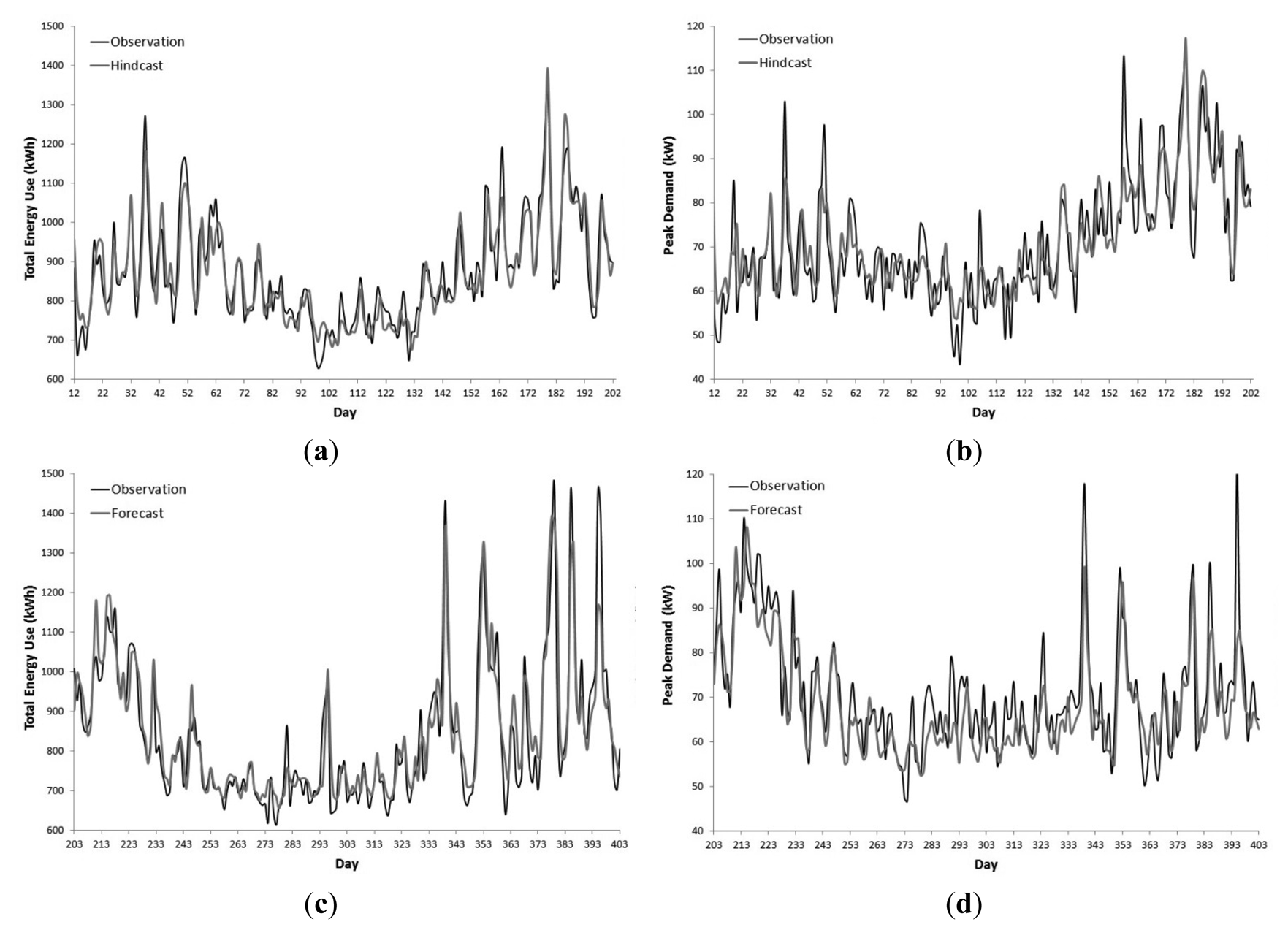
Figure 8 exhibits Phase 3's NDTEU and NPDPD hindcasts and forecasts for the hybrid models developed. For each of the hindcasts and forecasts it can be seen that the NN models' output accounts for the small fluctuations in demand. When the NN models' output is equal to the identified thresholds or above, the ARIMAX models' outputs are used instead such that the large spikes in demand are more accurately forecasted.

The use of both models as described above ensures that the better traits of the two techniques are utilized to provide an enhanced forecast of the residential LV network demand. The better hindcast and forecast fits are reflected in the reduction of RMSE. Forecasting demand in the LV network has received little research attention till recently, but power distribution companies now require bottom-up forecasting models that can handle the increasing penetrations of distributed renewable energy sources. LV network demand is notoriously volatile and requires hybrid techniques that can handle the large demand variance that occurs. This paper provides an attempt to create a suitable forecasting technique for this issue.

8. Conclusions

The objectives of this paper were to develop NDTEU and NDTD forecast models for the purpose of yielding information that a battery energy management system can use to schedule charging and discharging in a residential LV distribution network. Developing the models for a residential encounters additional challenges over larger subsections of the electricity supply and distribution due to increase in influence that individual customers have leading to greater variability and randomness. In turn, this paper aimed to present the significant variables which influence demand and compare the performance of the ARIMAX and NN modelling techniques to determine which is most applicable.

The most significant variable which influences residential LV distribution network demand was temperature. The demand response to temperature was observed to be parabolic in nature and accounted for half of the demand experienced. Other variables included in the models which helped to explain demand were DES, autoregressive terms, RH, interaction between RH and temperature and dummy variables for each day of the week. DES accounted for the long term seasonalities in demand by estimating the local mean throughout the data set.

ARIMAX and NN NDTEU and NDPD models were developed for each phase of the network. For the majority of the time series the NDTEU and NDPD hindcasts and forecasts were in line with observations. The NDTEU models were more accurate than the NDPD models due to the peak demand time series being more variable in nature. The NN models were slight gains over the ARIMAX models. Each modelling technique yielded benefits such as the ARIMAX models being better able to account for large spikes in demand and the NN models accounted for small fluctuations better.

Hybrid ARIMAX-NN models were developed to capitalize on the beneficial traits of both the ARIMAX and NN sets of models. The system operated by relying on the NN models to forecast demand and if the forecast was above a defined threshold, the ARIMAX forecast was used. The hybrid model better catered for both the small fluctuations as well as the large spikes in demand when compared to the standalone technique models for both hindcasts and forecasts.

Discrepancies between the models' hindcasts and forecasts occurred on days where there were large spikes in demand coinciding with exogenous shocks such as an unusual public holiday, a prolonged rainfall event or days with high maximum temperatures. Days with high maximum temperatures were investigated against model error and it was found that there were no statistically significant relationships.

To improve the accuracy of the models more research is required to investigate additional variables which influence customer behaviour. Future work will involve further investigations of customer behaviour, integrating the forecast models into an expert system which forecasts daily load profiles and developing a battery energy management control algorithm.

References

- Ackermann, T.; Knyazkin, V. Interaction between Distributed Generation and the Distribution Network: Operation Aspects. Proceedings of the IEEE/PES Transmission and Distribution Conference and Exhibition 2002, Asia Pacific, Yokohama, Japan, 6–10 October 2002; Volume 2, pp. 1357–1362.
- Lu, B.; Shahidehpour, M. Short-term scheduling of battery in a grid-connected PV/battery system. IEEE Trans. Power Syst. 2005, 20, 1053–1061. [Google Scholar]
- Bayod-Rujula, A. Future development of the electricity system with distributed generation. Energy 2009, 34, 277–283. [Google Scholar]
- Venu, C.; Riffonneau, Y.; Bacha, S.; Baghzouz, Y. Battery Storage System Sizing in Distribution Feeders with Distributed Photovoltaic Systems. Proceedings of the 2009 IEEE Bucharest PowerTech, Bucharest, Romania, 28 June–2 July 2009; pp. 1–5.
- Amjady, N.; Keynia, F.; Zareipour, H. Short-term load forecast of micorgrids by a new bilevel prediction strategy. IEEE Trans Smart Grid 2010, 1, 286–294. [Google Scholar]
- Oudalov, A.; Chartouni, D.; Linhofer, G. Value Analysis of Battery Energy Storage Applications in Power Systems. Proceedings of the IEEE PES Power Systems Conference and Exposition, PSCE ‘06, Atlanta, GA, USA, 29 October–1 November 2006; pp. 2206–2211.
- Hoff, T.; Perez, R.; Margolis, R. Mazimising the value of customer-side PV systems using storage and controls. Sol. Energy 2007, 81, 940–945. [Google Scholar]
- Gil, H.; Joos, G. Models for quantifying the economic benefits of distributed generation. IEEE Trans. Power Syst. 2008, 23, 327–355. [Google Scholar]
- Momoh, J. Smart Grid: Fundamentals of Design and Analysis; Wiley: Hoboken, NJ, USA, 2012. [Google Scholar]
- Nottrott, A.; Kleissl, J.; Washom, B. Storage Dispatch Optimization for Grid-Connected Combined Photovoltaic-Battery Storage Systems. Proceedings of the 2012 IEEE Power and Energy Society General Meeting, San Diego, CA, USA, 22–26 July 2012; pp. 1–7.
- Morais, H.; Kadar, P.; Faria, P.; Vale, Z.; Khodr, H. Optimal scheduling of a renewable micro-grid in an isolated load area using mixed-integer linear programming. Renew. Energy 2010, 35, 151–156. [Google Scholar]
- Hatziargyrion, N.; Dimeas, A.; Tsikalakis, A.; Lopes, J.; Karniotakis, G.; Oyarzabal, J. Management of Microgrids in Markets Environment. Proceedings of the 2005 International Conference on Future Power Systems, Amsterdam, The Netherlands, 16–18 November 2005; p. 7.
- Hernández, L.; Baladrón, C.; Aguiar, J.M.; Calavia, L.; Carro, B.; Sánchez-Esguevillas, A.; Sanjuán, J.; González, Á.; Lloret, J. Improved short-term load forecasting based on two-stage predictions with artificial neural networks in a microgrid environment. Energies 2013, 6, 4489–4507. [Google Scholar]
- Espinoza, M.; Joye, C.; Belmans, R.; Morr, B. Short-term load forecasting, profile identification and customer segmentation: A methodology based on periodic time series. IEEE Trans. Power Syst. 2005, 20, 1622–1630. [Google Scholar]
- Enslin, J.; Heskes, J. Harmonic interaction between a large number of distributed power inverters and the distribution network. IEEE Trans. Power Electron. 2004, 19, 1586–1593. [Google Scholar]
- Engle, R.; Mustafa, C.; Rice, J. Modelling peak electricity demand. J. Forecast. 1992, 11, 241–251. [Google Scholar]
- Darbellay, G.; Slama, M. Forecasting short-term electricity demand: Do neural networks stand a better chance? Int. J. Forecast. 2000, 16, 71–83. [Google Scholar]
- Ringwood, J.; Bofelli, D.; Murray, F. Forecasting electricity demand on short, medium and long time scales using neural networks. J. Intell. Robot. Syst. 2001, 31, 129–147. [Google Scholar]
- Taylor, J. Short-term electricity demand forecasting using double seasonal exponential smoothing. J. Oper. Res. Soc. 2003, 54, 799–805. [Google Scholar]
- Taylor, J. Triple seasonal methods for short-term electricity demand forecasting. Eur. J. Oper. Res. Soc. 2010, 204, 139–152. [Google Scholar]
- Taylor, J.; Buizza, R. Using weather ensemble predictions in electricity demand forecasting. Int. J. Forecast. 2003, 19, 57–70. [Google Scholar]
- Mirasgdis, S.; Sarafidis, Y.; Georopoulou, E.; Lalas, D.; Moschovits, M.; Karagiannis, F.; Papakonstantinou, D. Models for mid-term electricity demand forecasting incorporating weather influences. Energy 2006, 31, 208–227. [Google Scholar]
- Ko, C.; Lee, C. Short-term load forecasting using SVR (support vector regression)-based radial basis function network with dual extended Kalman filter. Energy 2013, 49, 413–422. [Google Scholar]
- Box, G.; Jenkins, G. Time Series Analysis: Forecasting and Control; Holden-Day: San Francisco, CA, USA, 1970. [Google Scholar]
- Australian Bureau of Meteorology. Climate Statistics for Australian Locations. Available online: www.bom.gov.au/climate/averages/tables/cw_040842.shtml (accessed on 22 July 2013).
- Gardner, R.; Dannenbring, D. Forecasting with exponential smoothing: Some guidelines for model selection. Decis. Sci. 1980, 11, 370–383. [Google Scholar]