The Real-Time Optimisation of DNO Owned Storage Devices on the LV Network for Peak Reduction


Abstract
: Energy storage is a potential alternative to conventional network reinforcement of the low voltage (LV) distribution network to ensure the grid's infrastructure remains within its operating constraints. This paper presents a study on the control of such storage devices, owned by distribution network operators. A deterministic model predictive control (MPC) controller and a stochastic receding horizon controller (SRHC) are presented, where the objective is to achieve the greatest peak reduction in demand, for a given storage device specification, taking into account the high level of uncertainty in the prediction of LV demand. The algorithms presented in this paper are compared to a standard set-point controller and bench marked against a control algorithm with a perfect forecast. A specific case study, using storage on the LV network, is presented, and the results of each algorithm are compared. A comprehensive analysis is then carried out simulating a large number of LV networks of varying numbers of households. The results show that the performance of each algorithm is dependent on the number of aggregated households. However, on a typical aggregation, the novel SRHC algorithm presented in this paper is shown to outperform each of the comparable storage control techniques.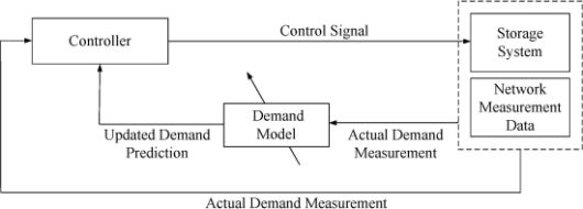
1. Introduction
As demand increases on the low voltage (LV) network due to changes in consumer behaviour and the electrification of transport and heating [1], the distribution network operators (DNO) will be forced to change the way in which they operate and reinforce this part of the network. Conventional reinforcement, either by upgrading existing cables and substations or adding new ones, is effective, but expensive. This need to update the existing infrastructure provides the opportunity for new methods of supporting the network, in particular, energy storage devices. Storage devices have many uses on the network [2,3]. In this paper, we focus on using such a device for the mitigation of peak loads in order to reduce peak load at the substation to avoid violating operating constraints on current and voltage and, as a result, to reduce network losses [4,5], to help support the distribution network. As smart meters appear on the network, DNOs will have greater visibility of the LV network. Load profiles on the medium voltage (MV) network are relatively smooth and often predictable, whereas LV network demand profiles are considerably more difficult to forecast, due to their stochastic and volatile nature [6]. Difficulty in producing accurate forecasts makes it considerably more difficult for storage on the LV to perform as successfully as has been shown, using traditional methods, on the MV network [7]. Most peak demand reduction algorithms in the literature mainly focus on the MV network. Storage control algorithms on the MV network can assume that an accurate forecast of future demand is available; this is not practical for the more volatile LV network. LV storage devices are still extremely expensive, but by controlling the storage device so that a DNO can achieve a better and more reliable demand reduction will, for a given battery size, have significant economical benefits in addition to the potential network benefits. Using a storage device on the LV network to get the greatest peak demand reduction cannot only help support a local LV constraint issue, but also help support network constraints on the MV (11 kV) network. For example, reducing a peak on the LV network can also help mitigate peaks and constraint issues on the MV network.
Two main methods for controlling a storage device are defined in the literature [8]. The first develops and deploys a plan based on historic network data to the storage device, and the second uses real time data available from the network to make a control decision; the latter is studied here in this work. Set-point control is the most basic form of this control and is traditionally how storage devices have been controlled [9]. Current research has shown that there are significant differences in performance that a storage device can achieve on the LV network, between the best possible demand reduction with a perfect demand model and when compared to the demand reduction achieved when being controlled using a set-point control algorithm [10]. Both the control methodologies described above run the risk of the shortage or surplus of the energy capacity in a storage device. Set-point control operates without any expectation of future energy demand, and therefore, its performance is significantly limited. It has been shown that using accurate demand forecasts to control storage can improve the performance [11,12]. Yu et al. have also shown that by using an optimization model, it is possible to incorporate storage and network constraints to control storage to support the network, reducing peak demand and network losses on the MV network [13].
In this paper, we present algorithms using real-time data available from the network, to make a control decision for the storage device on the LV network, firstly incorporating demand forecasts into the control of DNO owned storage devices and then treating the demand as a stochastic element in the controller.
Using model predictive control (MPC), also known as receding horizon control (RHC) [14], incorporating forecasts for the operation of network connected devices, has been proven to increase the systems performance. Molderink et al. present a three-step methodology, prediction, planning and real-time control, to control and manage domestic smart grid technologies [11]. In a follow up paper, the last step of the three step methodology is extended to include MPC; incorporating MPC into the methodology improves the results in the simulated examples presented in [15]. Adding MPC and, therefore, the ability to use real-time data to update predictions of future demand improves the ability to work around prediction errors, found in a volatile single domestic home, and has been shown in the system presented to improve the irregular behaviour of devices, which results in a more stable situation. The goal of the controller presented by Molderink et al. is to make optimal decisions given a certain objective, e.g., peak shaving or following a global objective (such as balancing supply and generation). The successful performance of MPC incorporating forecasts over traditional storage in smart grid applications can be found throughout the literature. For example, Beaudin et al. present a moving window algorithm for residential energy management [16]. The moving window allows the system to maintain an optimal schedule, as the forecast is updated. The algorithm is shown to outperform the baseline comparison algorithms, which do not use the moving window, and is more robust against forecast errors and fluctuations than the algorithms without a sliding window mechanism. As in Beaudin's work, Lampropoulus et al. develop a novel control scheme for demand response in the home [17], using MPC. The use of MPC is shown to successfully outperform conventional control when using the demand response for frequency control. These sets of work show why MPC is therefore a good candidate for the storage control technique presented in this paper. MPC has also been used to minimise emissions and the capacity of back up generators, which are used to balance intermittent distributed generation; again, the results show that by using a receding horizon approach can outperform a single time step optimisation [18]. Uncertainty with the MPC models has also been studied within [19–21] and for minimizing operational costs using electric vehicles [22]. It has also been shown that storage control incorporating uncertainty in the electricity market is possible using a receding horizon and no forecasts [23]; the work successfully reduces the impact of prediction errors using a heuristic-based approach. As forecasting on the LV network is difficult, the control of storage will be dependent on the accuracy of the forecast [12,24]. Therefore, this paper will, in addition, treat the demand as a stochastic process, considering stochastic control methods, as opposed to a deterministic forecast in an MPC controller, in order to compare the performance of multiple controllers for LV connected storage devices.
Stochastic optimization is a special subset of mathematical programming techniques that involves optimization under uncertainty. Wu et al. explore how, by using stochastic control methodologies, it is possible to help smooth wind generation using the storage element of plug-in electric vehicles [25]. A stochastic framework considering the uncertainties of how often the storage device is available and the errors in wind forecasts is presented. The results presented by Wu et al. in [25] show that the algorithm presented has the ability to smooth the volatile demand; the authors go on to propose that the algorithm could easily be adopted and implemented by DNOs. In 2009, Livengood et al. presented the energy box: a device that is able to control all connected devices in the home [26]. The energy box has multiple objectives, including load shifting and load valley filling. The energy box uses a stochastic dynamic programming control algorithm to make optimal control decisions. Similar stochastic control algorithms using forecasts in buildings [27] and micro-grids [28] can also be found in the literature showing how forecasts and a priori network data can successfully be incorporated into optimal stochastic control algorithms. Samadi et al. take into account load uncertainty and study demand response scheduling using variable pricing tariffs with successful results [29]. Recently, Murillo-Sanchez et al. created a stochastic optimization framework for the operation of an electrical network by a DNO [30]. The optimisation framework controls devices connected to the network, the framework's objective is to add the most benefit to the network through mitigating uncertainty and covering contingencies. Though the performance of the proposed system is not tested on any case studies, initial results show the successful convergence results of the optimisation.
It is important to note that not only has it been shown in some cases that studying the demand as a stochastic process can improve performance, but also using a receding horizon can improve the performance of storage control. Hence stochastic receding horizon control [31,32] will also be considered in this work. Nolde et al. in 2008 have shown how tuning the parameters of a stochastic model predictive control controller can lead to the successful medium-term scheduling of a hydro thermal storage system; the electric load and storage inflow are treated as stochastic processes [33]. Further, in the last few years, this control technique has also been studied for smart grid development in microgrid management [34], energy management systems [35,36] and for real-time market-based optimal power dispatch [37].
This paper will present and compare MPC and SRHC controllers for the control of a single DNO owned storage on the LV network. The objective of the controllers are to gain the greatest possible peak reduction as measured at the LV substation. The algorithms will be comprehensively tested to verify their suitability for LV storage control by varying the number of individual domestic customers in a demand aggregation and testing the algorithms on large data sets, using real network data and, therefore, introducing real demand errors. This realistic demand error and varying aggregation size is important to study, due to the volatile nature and varying demand models on this part of the network. The smart meter data used in this work have been supplied by Ireland's Commission for Energy Regulation and is openly available on-line via the Irish Social Science Data Archive [38]. Therefore, the paper has multiple contributions: the work studies and presents novel controllers for the control of the LV network connected DNO owned storage device's, where the objective is to achieve the greatest possible peak reduction, given a pre-defined storage device. The SRHC controller treats the demand as a stochastic process and formulates a scenario tree based on a priori demand data. The research presents a technique that studies the historical variance of the demand in order to find the number of nodes per time step of the scenario tree and a bin-based methodology to assign the nodes probabilities and demands from the a priori data. Unlike the current literature, which often negates the LV network, the algorithms performance for different sizes of demand aggregations, incorporating actual errors found on the LV network between the actual and forecasted demand, will also be studied, as well as studying the performance of the algorithms for a large number of demand aggregations. The paper has the following structure. The next section, Section 3, will describe the storage system and the demand model. Sections 4 and 5 will introduce the MPC and SRHC controllers, respectively. Section 6 will present a comprehensive set of results varying from an individual aggregation, multiple sizes of demand aggregations and large data sets using demand aggregations found on the LV network. Finally, the conclusion is presented in Section 7.
2. The Energy Storage System and LV Network Demand Model
This work addresses the on-line peak reduction storage control problem as described in [10,11,39] and discussed in the previous section. This section will define the storage system and introduce the characteristics of the demand profiles found on the LV network. The following two sections will then introduce the control techniques used to control this system. The storage system used in this work is shown in Equation (1) and is similar to that found throughout the literature [18,40]. Typically, the control of the energy storage device is given in terms of the power flow (Ps) in kW's, and the energy stored is given as Psτ in kWh's, where τ is the duration of the time period in hours. However, in this paper, the increase or decrease of the energy stored in the storage device is given as δS(k) = Ps(k)τ = SOC(k) − SOC(k − 1). The change in energy, δS, between time steps, can be positive or negative and represents the increase and decrease of the energy stored in the storage device; when δS is negative, the energy in the storage device has decreased, and when δS is positive, the energy in the storage device has increased. The system dynamics are subject to maintaining a maximum and minimum state of charge, SOCmin and SOCmax, and the maximum increase and decrease in energy in the storage device between time steps, and . These constraints are represented in Equations (2) and (3), respectively. The algorithm also takes into account the storage devices efficiency and standby losses, η and µ, respectively [10], as the change in energy of the storage device between time steps has been combined into one variable; when δS is negative, the storage devices efficiency is , as shown in Equation (4). It is customary to define the SOC quantity as a value between zero and one; however, in Equation (1), as in [41], the state of charge at the end of each period is determined by the previous period's SOC level and the increase or decrease of energy in or out of the storage device (δS) at the current period.
As described in the previous section, aggregated individual smart meter profiles, DiA, where i is an individual, domestic customer, are used to represent the demand profile, DA. Equation (5) shows the aggregated demand.
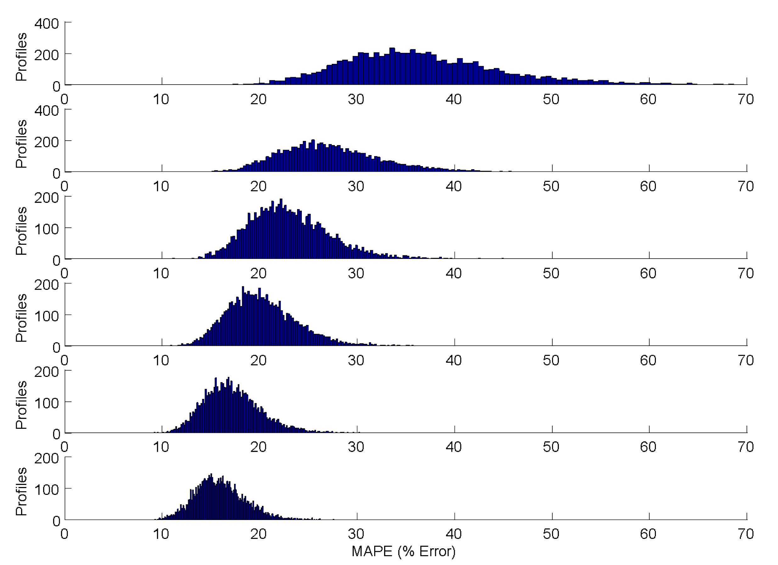
The objective of the research presented in this paper is to minimise the peak demand (DA), which is measured in real time on the network, using the storage system previously defined. This demand aggregation, DA, is comparable to a storage system with substation monitoring, where the total demand consumed on a feeder is used to make future control decisions for the storage device. As the real-time demand data becomes available, a model of the demand is updated, and the forecasted demand and storage device states are fed to the controller. As previously discussed, the LV network is volatile and difficult to predict; therefore, developing this forecast is difficult. Another complex feature with regards to the demands' behaviour, which is important to study for understanding the robustness of an LV storage control technique, is how different numbers of demand profiles in a demand aggregation affects the potential accuracy of a forecast. The forecast used in this paper is based on recent developments in forecasting at the household to small aggregations of household demand level [6] and will be discussed in the following section. A typical single phase on the LV network can have between five and 40 customers; therefore, Figure 1 shows how the mean absolute percentage error (MAPE), between the actual and forecasted demand, varies for different demand aggregation sizes.
Figure 1 shows five histograms, each showing the MAPE error between the actual and forecast demand of 1000 daily profiles of demand aggregations, where the aggregation size is varied in size from five to 35 customers. As the number of demand profiles in an aggregation increases, the accuracy of the aggregated forecast increases. This behaviour is expected, as the law of large numbers comes into play at larger aggregations. Therefore, in this paper, as there is a significant difference between the demand characteristics with different aggregation sizes, all the algorithms are tested on multiple sizes.
At each time step, k, the controller is required to make a control decision by using a future prediction of the demand and minimising a cost function. The work in this paper will present and compare two techniques: the first described in Section 4, model predictive control (MPC), uses a deterministic forecast based on historic data embedded into the algorithm to control the storage device. The second control technique described in Section 5, stochastic receding horizon control (SRHC), uses the historic data and stochastic optimisation to study the probability of potential future demand routes occurring, and similarly, a cost function is used to find the optimal control decision. The energy storage model described above in this section is kept constant in each control technique discussed in this paper.
3. Model Predictive Control (MPC)
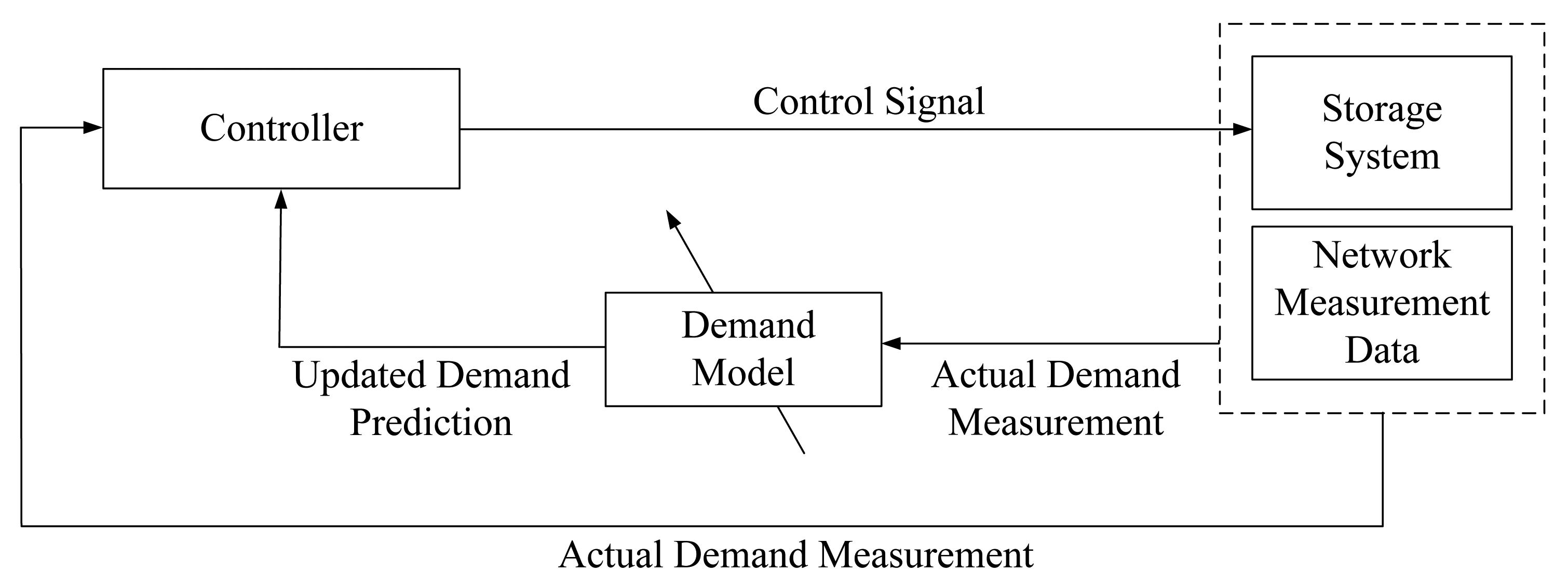
The controller is formulated as a model predictive control (MPC) problem. MPC, also known as receding horizon control, refers to a class of control methods that compute a sequence of decision-variable adjustments over a future time horizon iteratively based on an underlying optimization model [14]. Figure 2 shows the control loop for the system. The output, the measured demand, is fed back into a model of the demand, and based on an updated demand prediction, shown in the inner loop for a pre-defined horizon size, and the actual demand shown in the outer loop, the controller derives the control signal by minimising a cost function.
The cost function used in this work is shown in Equation (6). This cost function will minimise the maximum peak in each simulation of N samples of k, where DA is the original demand profile and where δS, the decision vector, is the increase and decrease of energy in the storage device.
At the current time step, k, the controller gets the forecast between k and k + Hp, where Hp is the prediction horizon and k + Hp ≤ N. Using this model, the controller computes the optimal control signal and applies the control input to the system. The process is repeated at each time step k + 1; therefore, the controller uses the forecast given for each time k + 1 to k + 1 + Hp, where k + 1 + Hp ≤ N, to derive the control signal. The performance of an MPC problem strongly depends on the accuracy of the forecast. In this work, the forecast is generated using a recently developed forecasting technique [6]. As previously discussed, individual smart meter data is forecast and then aggregated. Peak usage is likely to differ by a few half hours earlier or later in a normal household, due to natural irregularities in behaviour, and therefore, any forecast to be used for the control of a storage device must allow for these small changes. The forecasting technique used in this paper assumes week to week regularity, but allows for small adjustments in the behaviour. As the number of demand profiles in an aggregation increases, the accuracy of the aggregated forecast increases. In Section 3, it was shown, in the data presented, that the average MAPE for an aggregation of 15 demand profiles is 22%. The average error decreases to 14% in aggregations of 35 demand profiles; this trend is due to the law of large numbers [42]. Another important parameter to select in the MPC formulation is the size of the horizon, as the longer the horizon, the more computationally heavy the control becomes, but the further in advance the controller can plan. The Results section, Section 6, presents a technique for finding the horizon time for peak reduction storage control. It has been shown that planning ahead is vital when controlling storage [11,12,39], and to highlight this point on the single phase of the LV network, the performance of the MPC controller is compared to a standard set-point controller in Section 6, where the set-point is found from a priori demand data. Current smart grid literature has begun to explore the benefits of stochastic control and, therefore, treating the demand as a stochastic element. Given the volatility of this part of the network and the difficulty in predicting it, the next section of the work will take the deterministic MPC problem and formulate the problem as a stochastic receding horizon control problem.
4. Stochastic Receding Horizon Control (SRHC)
The MPC problem is now formulated as a stochastic optimisation problem with a receding horizon [31,32]; the control loop has the same structure to that shown in Figure 2, with a modified controller, which will now be introduced. As stated in Section 1, studying demand as a stochastic process has shown significant benefits in the control of network connected devices. Traditionally stochastic programming does not use a receding horizon, though, as previously discussed in Section 2, using a receding horizon can have a positive impact on the performance of storage control; therefore, making SRHC an ideal candidate for the volatile and difficult to predict nature of the LV network. The SRHC problem in this work is defined as the expected performance (
 [ . ]) of a given cost function, J, and δS the previously defined control signal, as shown in Equation (7), where ω denotes a stochastic variable described below.
The problem solved in this paper, incorporating the cost function introduced in the previous section, is shown in Equation (8), where the demand, DA(ω), is treated as a stochastic variable and J = max (DA(ω) + δS)}2. The objective function in this form with the constraint Equations (1)–(4), previously introduced, forms a multi-stage stochastic programming problem. The problem is solved by approximating the true problem shown in Equation (8) by discretising the problem where k ∈ {1, 2…, N − 1, N}. The true continuous problem is therefore transformed to a deterministic linear optimisation problem and presented later in this section.
A scenario tree is used to approximate the continuous problem. Typically, these trees are developed based on heuristic rules used to develop potential future scenarios or selected using data based on the environment's historic behaviour; the latter is used in this work. The tree is formulated using the historic half hourly data, and the routes of potential future demand and their associated probabilities are found from this a priori data. Section 5.1 will present a technique to select the number of nodes per time step based on the variability of the historic data at a specific time step. Section 5.2 will then show how to find the associated demand and probability, for each node, occurring at future time steps based on the historic demand data. Once the tree has been formulated and all nodes assigned a demand and probability, the nodes and associated routes across the tree are used to formulate a linear programming problem. Solving the linear programming problem will assign each node a control signal and, therefore, the control signal to be applied at the current time step.
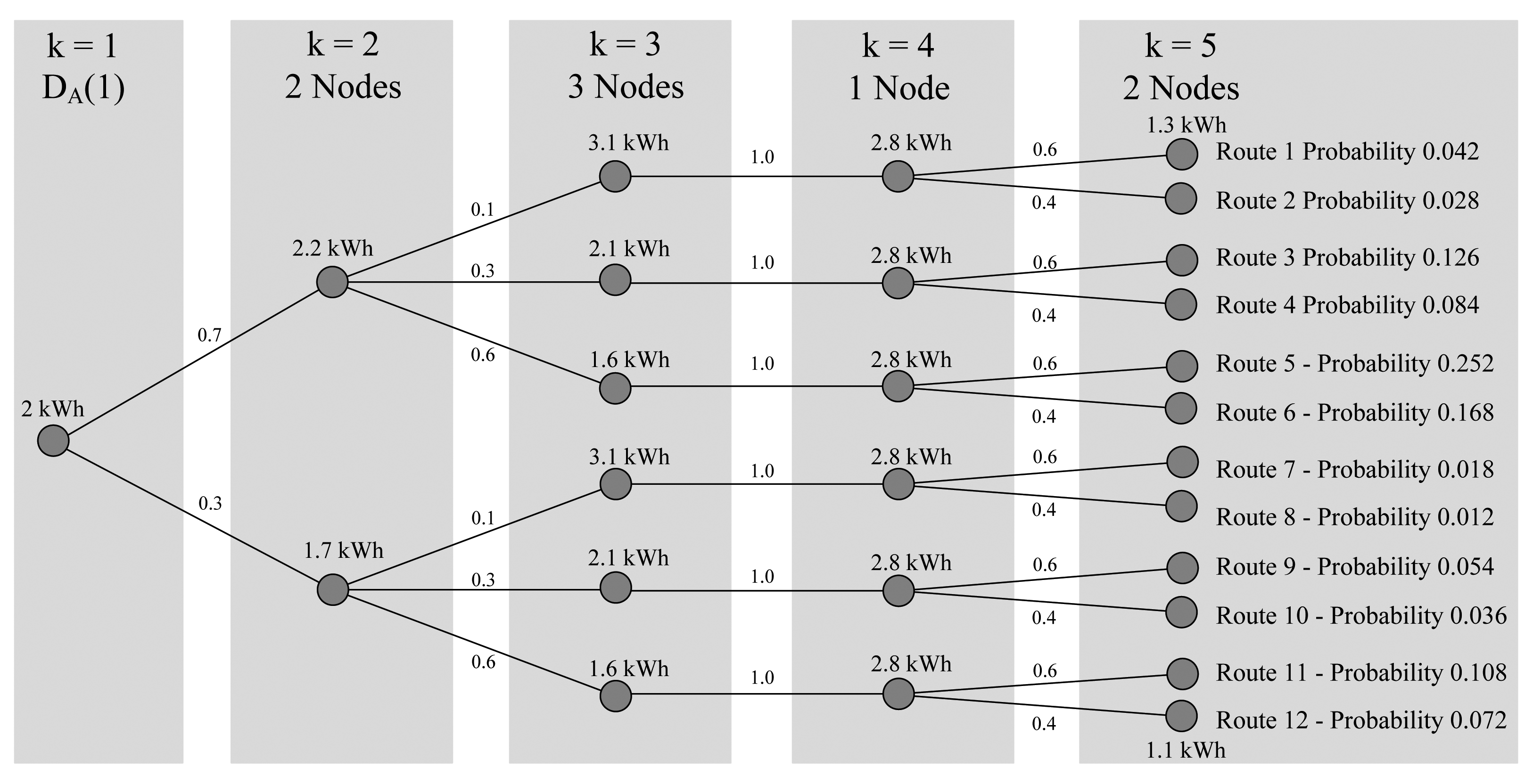
Figure 3 shows an example of a simple scenario tree, where each node of the tree is assigned a demand and probability. A control signal is assigned to each node once the problem has been formulated as a solvable optimisation problem. Previous work has shown that selecting the length of the horizon and number of nodes in the tree is critical in the performance of SRHC [33]. In Figure , at time Step 1 (k = 1), the demand is 2 kWh. In this example, at k = 2, two nodes have been selected; the probability of the demand being 2.2 kWh is 0.7, and the probability of the demand being 1.7 kWh is 0.3 at Nodes 1 and 2, respectively (see Section 5.2). At k = 3, three nodes have been selected, and at k = 4, the deterministic result is chosen with a probability of one. Figure 3 shows how the tree is built up, and the probability of each complete route occurring is shown. The notation used to describe the SRHC in this section is now defined. will denote the control signal, δS, at time k for node n of the scenario tree, the demand at time k for node n of the scenario tree and Pn(k) the probability at time k for node n of the scenario tree. During the optimisation, it is also useful to define vectors that contain the control signal, demand and probability along a route, r, of the tree; therefore, is defined as the control signal vector of δS along route r of the scenario tree, DrAR(k) is the demand vector, Da, along route r of the scenario tree and is the probability vector along route r of the scenario tree. In Section 6, the Results section, it is shown that the MPC deterministic controller described in the previous section requires a horizon time of at least 7 h (14 half hourly time samples). Table 1 shows that there is a significantly larger number of nodes and routes required to formulate the scenario tree when the number of nodes is increased by just one. For example, simply increasing the number of nodes per time step from two to three increases the number of possible routes from 16,384 to 7,174,453 when a 7.5-h horizon is used. Therefore, to overcome the problem of large trees, Section 5.1 introduces an algorithm to select a different number of nodes at individual time steps. The table shows that by varying the number of nodes in this way, this will lead to considerably smaller trees where the optimal control signal for a specific tree can be computed faster. From Table 1, it is possible to see by reducing the number of nodes per time step that the problem becomes intractable and, therefore, requires additional approximations. Similar to [30], by setting a small number of nodes in a time step, the problem is restricted to the center of the tree. In the work presented in this paper, as with [30], tree reduction algorithms found in the literature are used to reduce the number of variables in the optimisation problem [43].
As opposed to attempting to solve the continuous problem previously shown in Equation (8), the discretized approximated problem is now solved using linear programming. The discrete problem is shown in Equation (9), subject to the system in Equation (11) and system constraints (4), (12)–(15). Equation (9) contains the cost function used in the deterministic MPC controller shown in Equation (6); however, as the SRHC controller incorporates many potential demand routes, the expected value of each of the routes is used. As with the MPC formulation, Equation (9) finds the , though, as shown by the notation in the SHRC formulation, this is multiplied by , the probability of each route r occurring. The value for each route up to route T is then summed to return the expected value. This is shown in the expanded version of Equation (9) in Equation (10). Therefore, Equation (9) represents the discrete solution to the continuous cost function shown previously in Equation (8), and the optimisation vector is shown in Equation (16). As the demand is to be reduced throughout the complete time period and not summed per time step, throughout the period, the optimisation function uses the demand and probability notation, incorporating each complete route of the scenario tree.
This can be expanded to:
The optimisation vector is given by:
4.1. Selecting Nodes
The number of nodes per time step are selected by analysing the a priori data (HD ∈ ℝdT×N) and studying the variance (V ∈ ℝ1×N) of this data per time step k. When the variance is low, at off-peak times, the demand is easier to predict, whereas at on-peak times, when the demand is typically more volatile, the variance has a larger value. On the LV network, it would not be correct to assume that ‘off’ and ‘on’ peak would be at a traditional time, as can be seen on larger aggregations of customers; therefore, a specific temporal decision is not made, as with other storage control algorithms in the literature. By only selecting a small number of nodes when the demand is known in advance and where historically the demand varies only slightly, this part of the stochastic problem can be approximated and simplified as a deterministic model with one scenario: the forecasted demand value at time k is used; this is similar to assumptions with solar radiation and demand profiles explored in [44]. The algorithm is shown below (Algorithm 1).
| Algorithm 1: Selecting the nodes used in the scenario tree per time step. |
1. Initialise: HD, NodesMin, NodesMax ,
 ,d ,d |
| 2. Set V ← GetVarianceVector(HD, d) find variance vector for day d from historic data |
| 3. find variance thresholds to define bin limits |
| 4. For k = 1 to N samples in daily demand profile |
| 5. For t = 0 to (NodesMax − 1) loop through variance bins |
6. If {(
 × t) ≤ D(k) ≤ (
× (t + 1))} Check if demand is in bin × t) ≤ D(k) ≤ (
× (t + 1))} Check if demand is in bin |
| 7. Set
(k) = t + 1 assign number of nodes at time k |
| 8. Exit For Loop |
| 9. End If |
| 10. If D(k) > max(V) check if demand is outside maximum variance bin |
| 11.
(k) = NodesMax assign maximum number of nodes |
| 12. End If |
| 13. End For |
| 14. End For |
4.2. Sampling from the Historic Data
Once the number of nodes per time step
has been selected, the probability and demand of each specific node is found from the a priori data. Monte Carlo methods are typically used to formulate the scenario tree and to sample from a continuous distribution for stochastic optimisation. The approach adopted in this paper is similar to those that allow the discrete samples to keep the shape of the continuous distribution. Randomly sampling from the continuous distribution was not found to be a suitable option for this application, as compared to other stochastic control-based algorithms, only a small number of nodes can be used per time step, meaning a random sample could poorly represent the continuous distribution. An algorithm is used to find the probability and demand of the nodes in
(k). The algorithm uses a bin system to formulate the scenario tree from the a priori data; a bin is notated as b, and one bin is used to represent each node in
(k). The maximum number of bins, bmax, is equal to
(k) at time k; the bin size, bsize, is then found using Equation (17), where HD is a matrix of prior demand data HD ∈ ℝdT×N.
5. Results and Discussion
This section will present results from the previously discussed deterministic and stochastic-based control algorithms. First, a specific case study will be presented; then, the MPC and SRHC algorithms will be tested on larger data sets of varying aggregation sizes. Throughout this section, the algorithms will be compared to two algorithms found in the literature and used to benchmark DNO owned storage devices [10]. The first is set-point control [9], where, as per [10], the set-point value is determined from historical data. Set-point control is the standard control technique used to control storage devices on the network, where the demand, or voltage and frequency, etc., is compared to a set-point. The set-point in this work is defined as a value in kWh and is typically either a value set by a DNO as a maximum network constraint or found from the a priori data, as in this paper. The algorithm also requires predefined charge and discharge rates for the storage device. The algorithm then compares the current demand at each discrete time step to the predefined set-point, and the storage device makes a decision as to charge or discharge. If the demand is below the set-point, the storage device will charge until the storage device capacity is full; else, if the demand is above the set-point, the storage device will discharge at the set rate, until the storage device capacity is empty or the demand goes below the set-point again, therefore reducing the demand up the network from the storage device. As discussed in the Introduction, this set-point control algorithm is simple, but is fundamentally limited, as it operates without any knowledge of what is expected to happen in the future. The second comparison is to the best possible demand reduction a storage device can achieve for a given known demand profile and pre-defined storage device. This algorithm uses the constrained optimisation problem shown in Equation (6), subject to constraint Equations (1)–(4), with a perfect demand model, to find the best possible demand reduction.
5.1. A Specific Example
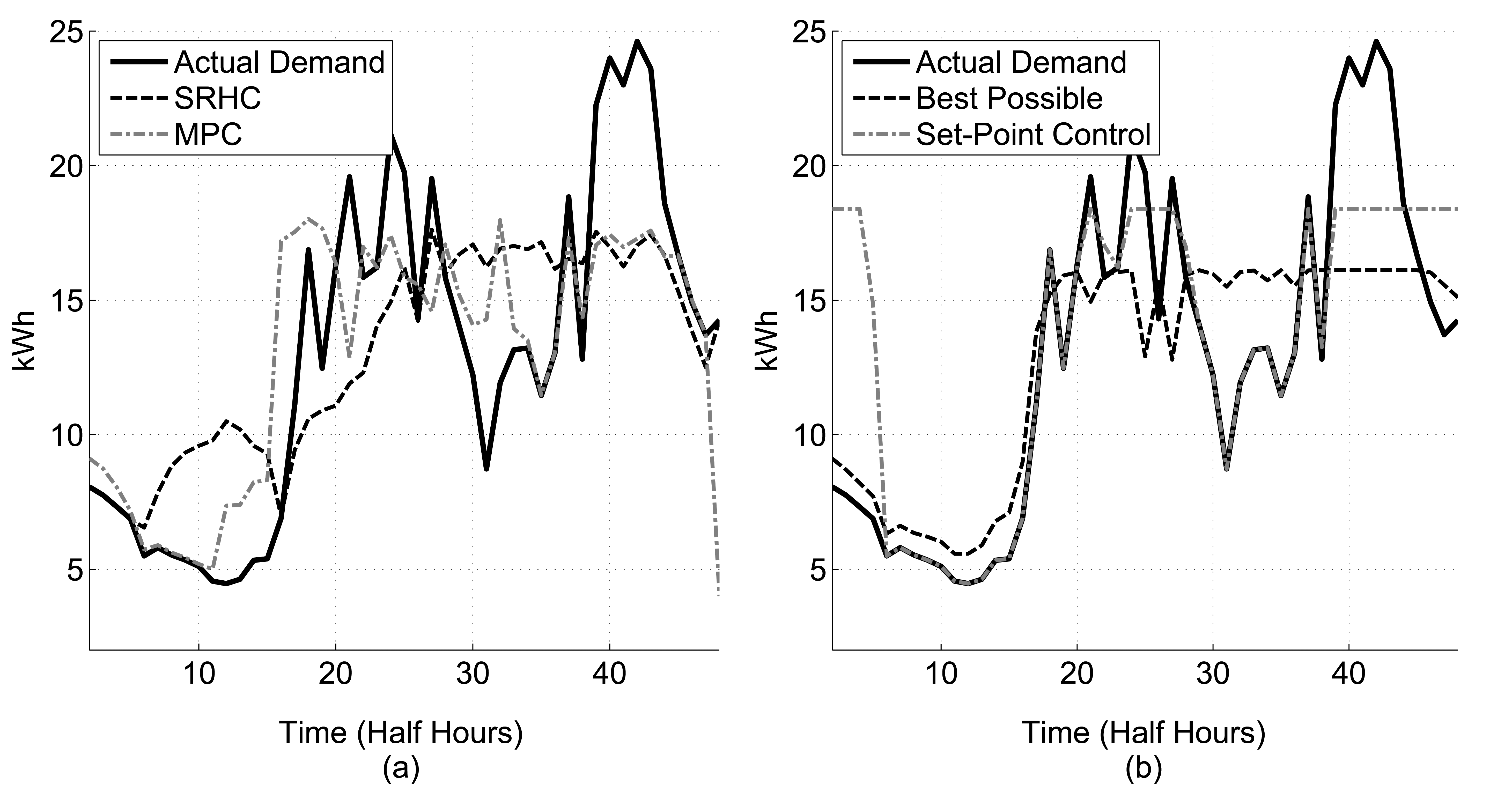
The energy use of forty homes, recorded by smart meters, was aggregated to represent a realistic single phase of a feeder in the distribution network and validated against historical substation data. A period of 15 weeks was considered and split into 14 weeks of historical data; the forecasts were based on the first 14 weeks, and day one of week 15 is presented in Figure 4. The following parameters were used in this example: Asize = 40, N = 48, SOCmax = 50 kWh, SOCmin = 0 kWh, and (a discharge rate of 80 kW and a charge rate of 100 kW, given half hourly smart meter data) over a sample (k). The storage device efficiency is not the focus of this research; therefore, η = 1 and µ = 0. The MPC algorithm uses a prediction horizon, Hp, of 12 samples of k. The SRHC algorithm uses the following parameters: Nodesmin = 1, Nodesmax = 4 and the same prediction horizon as for MPC. The results showing the comparison of the four algorithms are shown in Figure 4. SRHC outperforms set-point control and MPC in this example: SRHC achieves a 28.4% demand reduction; MPC 26.8%; and set-point control a 25.2% demand reduction. The set-point is set at 30% of the maximum peak from the previous week; this percentage achieved the greatest peak demand reduction from the previous week's demand profile when using the set-point controller. Using a percentage of a priori data to find the set-point is typical of set-point control algorithms presented in the literature. If a perfect model of the demand had been used, a demand reduction of 34.6% could have been achieved. As the SRHC algorithm uses historic variance to decide on a charging strategy, the storage device charges to full capacity by the 15th half hour, minimising the risk of charging on a peak. In contrast, the deterministic MPC algorithm, in fact, has introduced a new peak at the 19th half hour, as the variance data is not available to the deterministic algorithm.
5.2. Time Series State of Charge (SOC) Evolution
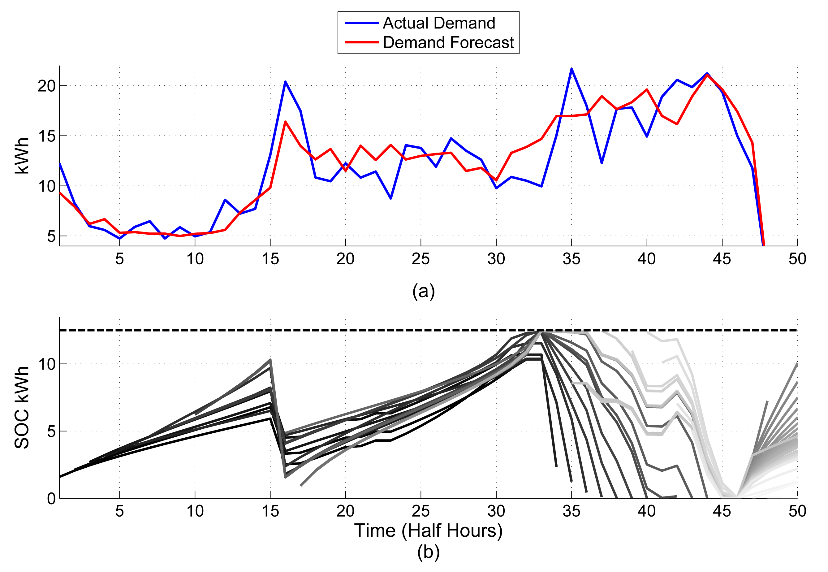
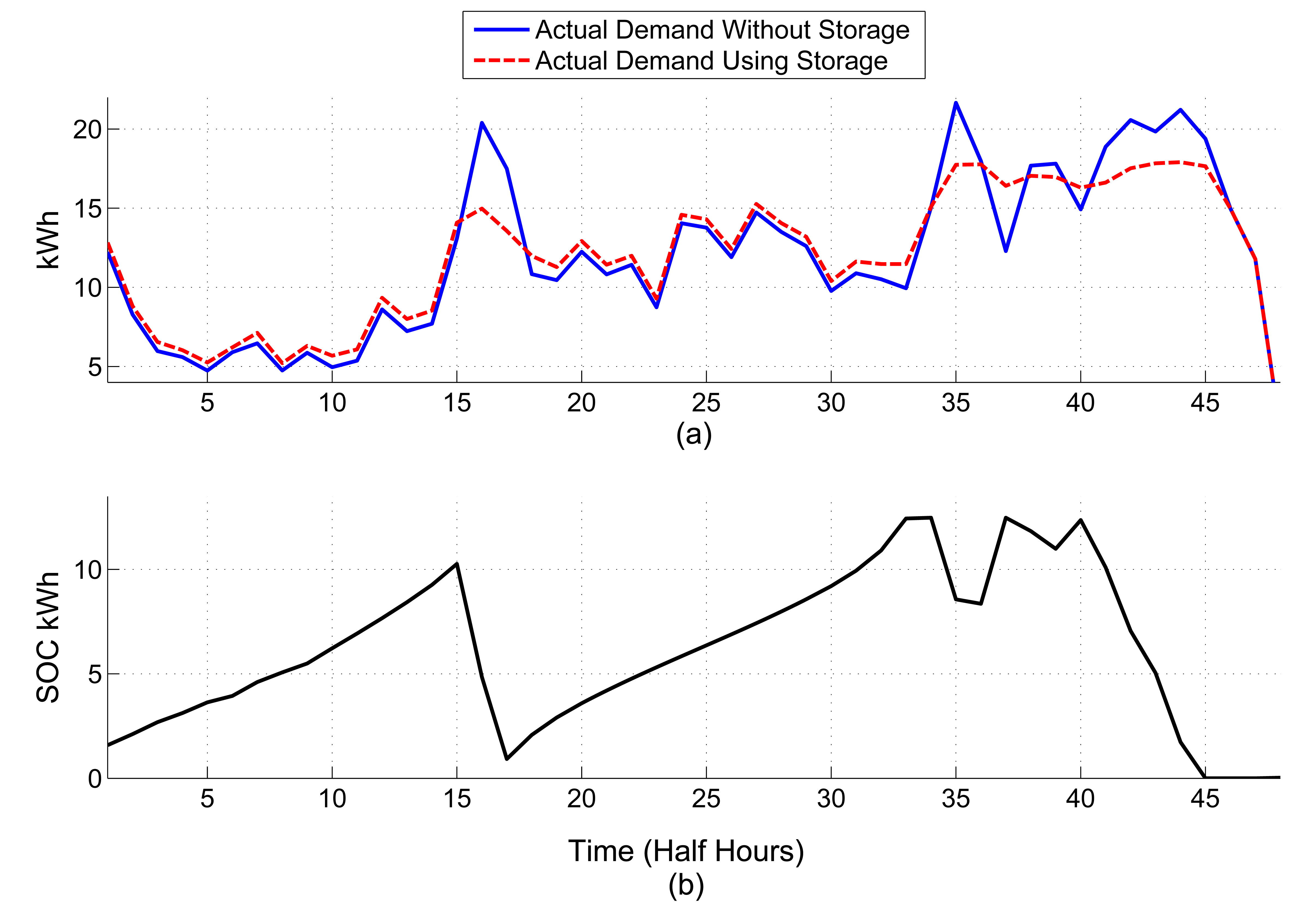
This section will show how the SOC varies as the horizon moves across a daily demand profile. Thirty daily household demand profiles have been aggregated (ASize = 30), and the result of the deterministic controller is evaluated. Figure 5 shows the forecast and actual demand profile for the aggregated demand. The following parameters were used in this example: Asize = 30, N = 48, SOCmax = 12.5 kWh, SOCmin = 0 kWh, and over a sample (k). The initial storage device SOC = 1 kWh. A large horizon size of 15 h (HP = 30) is used in order to show how the SOC evolves over time. The final result of the MPC controller is shown in Figure 6. The algorithm achieves a demand reduction of 17.3%; as a comparison with a perfect forecast, the algorithm achieves a demand reduction of 19.1%. Figure 5 shows the evolution of the SOC and the control signal, δS. The figure shows when there are larger errors between the forecast and the actual demand profile. For example, at the 17th half hour and at the evening peak time from the 35th half hour, the SOC profiles vary more between horizons than when the forecast is more accurate. The result shows that the algorithm in this example is able to deal with the larger errors between the forecast and actual demand, though with a more accurate forecast, the SOC evolution is smoother. Section 6 will now go on to evaluate the effect of the horizon size, of the MPC and SRHC controllers, on the demand reduction.
5.3. Varying the Prediction Horizon (Hp)
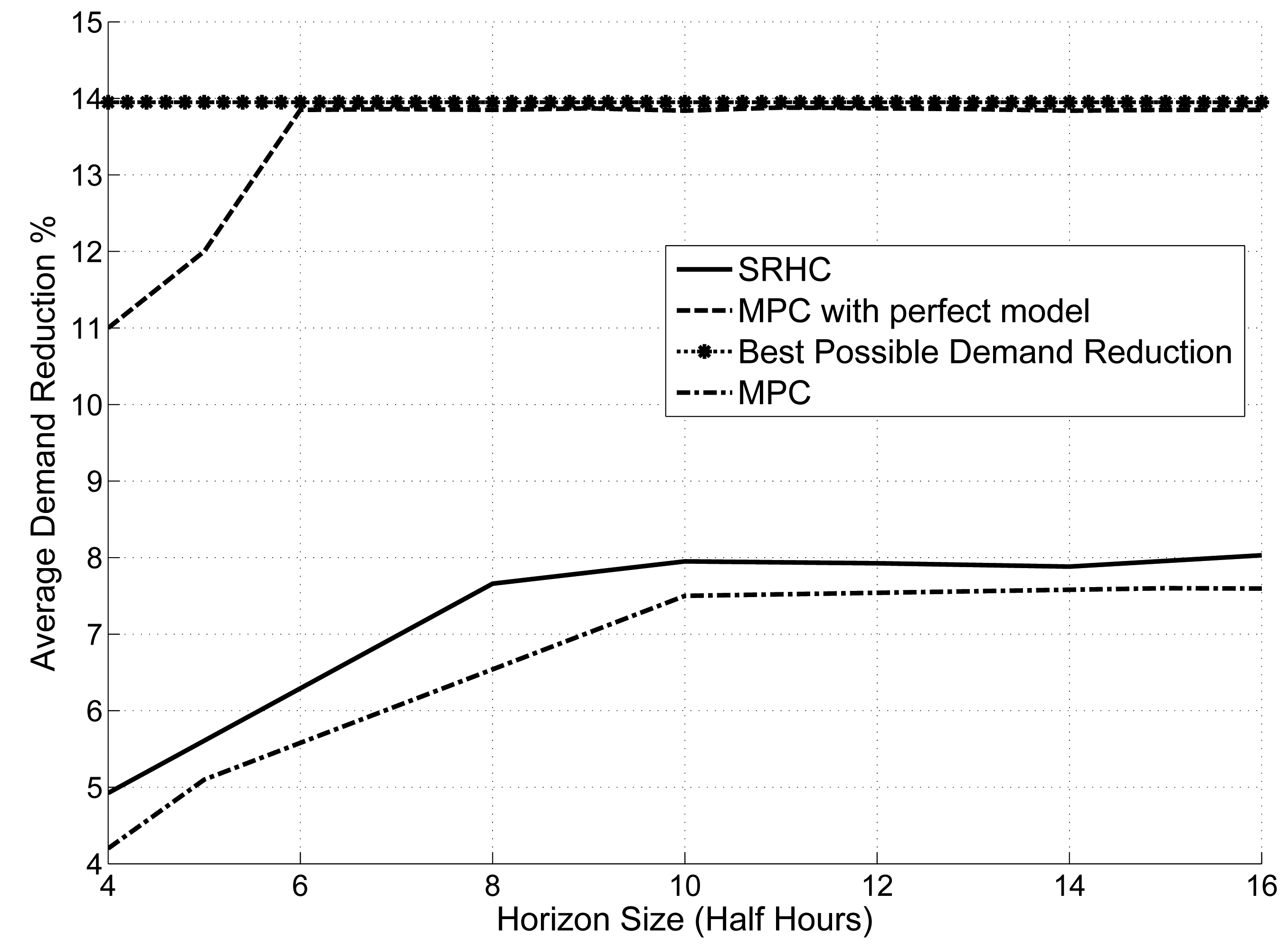
As discussed in Sections 4 and 5, the horizon size is an important parameter required in both algorithms presented in this paper. To compare the performance of the system vs. the algorithm's horizon size, the algorithm is run over multiple study cases and the results presented. Figure 7 shows the results of running the algorithms on 500 demand aggregations when the storage size is normalised per simulation and an aggregation size of 35 individual demand profiles is used; Asize = 35. The storage size is normalised between demand aggregations and simulations by sizing the storage at 25% of the maximum peak of the demand profile. Therefore, for a given demand profile, DA, of 48 half hourly samples, SOCmax = 0.25max(DA) kWh, , over a sample (k).
Figure 7 shows the average performance of the algorithms over all 500 daily simulations. The best possible average demand reduction, given perfect knowledge of the demand, is 13.95%. This is used as a benchmark performance of the MPC algorithm with a perfect demand model. The average demand reduction of MPC with a perfect demand model converges to within 0.7% of the best possible demand reduction; a slight difference is expected due to the restricted horizon size using the MPC algorithm. The MPC with forecasted demand and SRHC algorithms converge at approximately the 11th half hour for this example. The horizon size is not increased beyond 16 half hours, as all algorithms can be seen to converge, and as described in the previous section, the computation time increases exponentially for the SRHC algorithm. Therefore, for the set of data presented, a horizon size of 6 h (12 half hours) will be used for all daily simulations using the MPC and SRHC algorithms. The result shows that when setting the horizon size too small, the minimization occurs in times of lower demand, for example where the peak load within the window is not in a critical region when the demand is at its highest throughout the day. Therefore, setting the horizon time too small may mean the storage device is operating when not necessary and, as a result, wears the storage device out without achieving the greatest possible reduction in demand throughout the required daily period. In contrast, having a larger window, though computationally more expensive, allows the storage device to plan ahead for the larger peaks in the daily period, allowing the storage device to achieve a greater demand reduction throughout the day.
5.4. MPC vs. Set-Point Control: Varying Aggregation Size
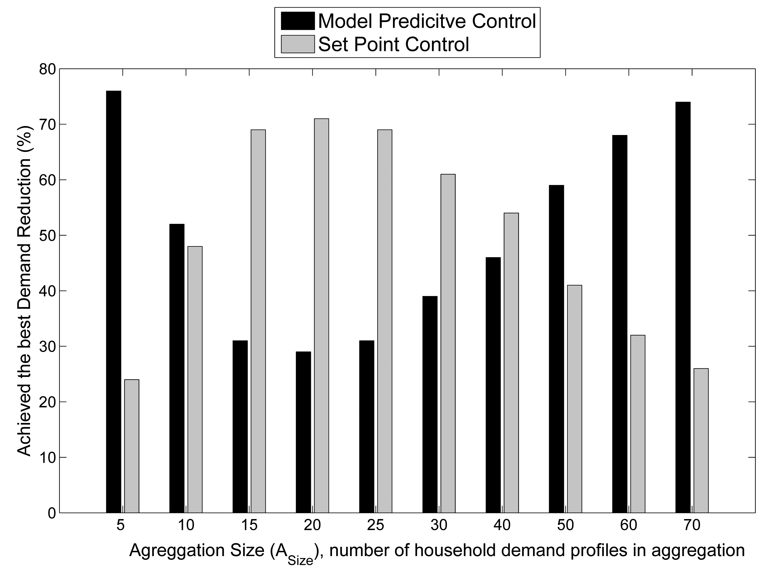
The MPC algorithm is now compared to a set-point control algorithm, where the set-point has been calculated from the previous day's demand profile. The two algorithms, MPC and set-point control, are run on the same demand profile using the same specification storage device. The results show the total number of times, as a percentage, that each algorithm achieved the greatest peak demand reduction across all simulations. Each aggregation size contains 7000 simulations, made up of 500 demand aggregations over 14 days randomly selected across a year's worth of data. The result for when the aggregation size is varied from five to 70 customers is shown in Figure 8. As previously discussed, as the size of an aggregation increases, the forecast becomes more accurate, and from aggregation sizes of 50 and above, the MPC algorithm begins to out-perform the set-point control algorithm. Due to the volatile nature of smaller aggregation sizes, set-point control using the set-point from the previous day performs poorly. It is difficult to consistently find a set-point that will achieve the best possible demand reduction. As the storage device size has been kept constant throughout all of the simulations, the results show that MPC, without providing any additional set-points, is able to outperform set-point control in aggregations sizes above around 40 customers as the demand model becomes more accurate. The figure shows that neither algorithm consistently outperforms the other. The results do show that the MPC algorithm could improve the performance of DNO storage devices for larger aggregations of demand and that as the demand model becomes more accurate, as newer more accurate forecasting techniques are developed, the performance of the MPC controller in smaller aggregations is expected to improve. For example, the forecasting technique used in this paper does not take into account weather variables that have been shown to improve the accuracy of demand forecasts [45]. In several state-of-the-art smart grid studies, where the control of devices on the network has been comprehensively tested, as in this work, it has also been important to select the correct algorithm based on the demand characteristics. Xu et al. concluded that it is important to study the application in detail before selecting a control technique [44]. This result confirms, for the data presented, that selecting the correct storage control technique for peak reduction, using DNO owned storage devices to achieve the best possible demand reduction, will depend on the accuracy of the forecast and the variation in actual demand reduction that can be achieved.
5.5. SRHC, MPC, Set-Point Control and Perfect Demand Model
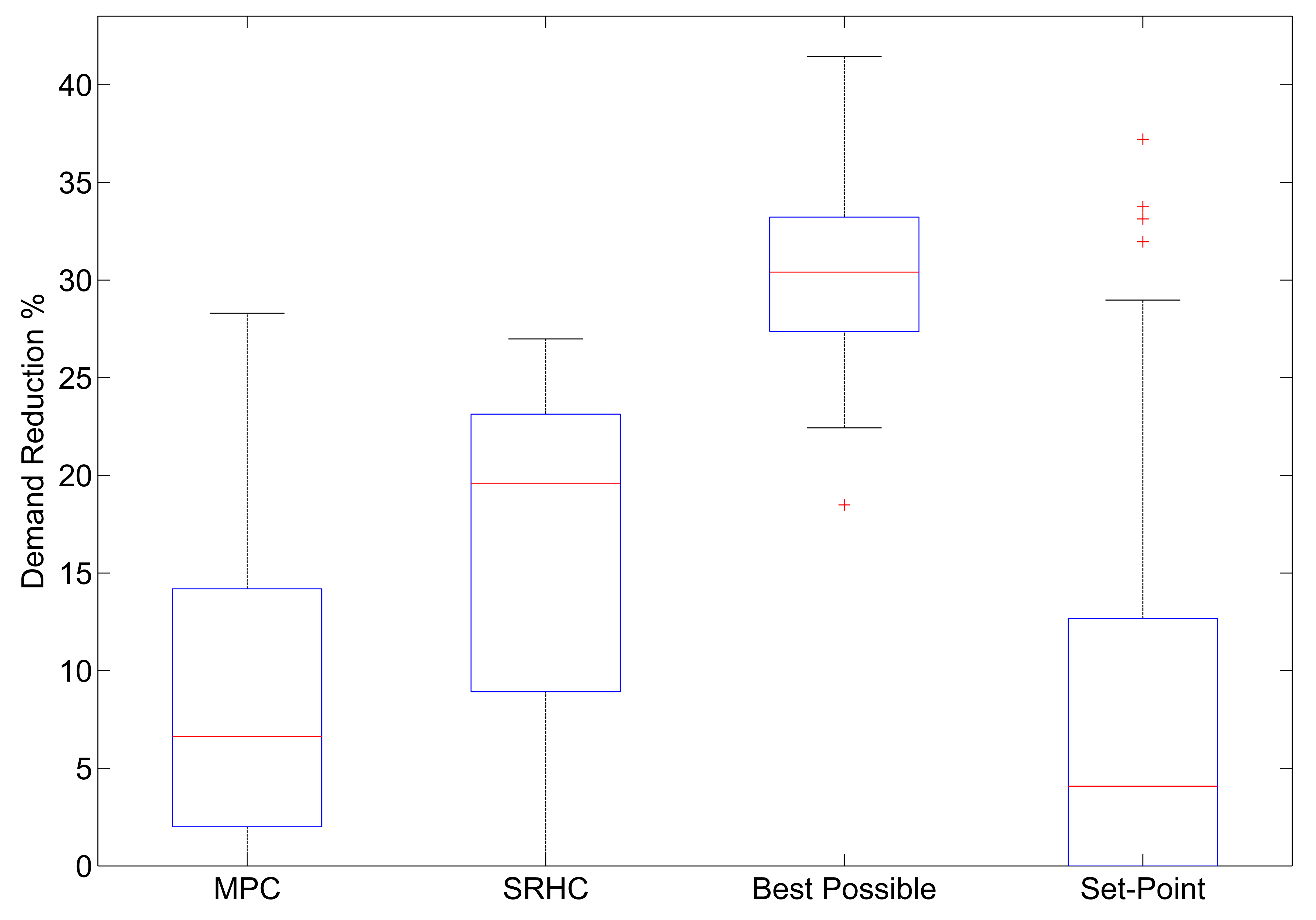
All algorithms discussed in this paper are now compared. An aggregation size (Asize) of 40 demand profiles has been used, which is representative of the typical number of customers found on the single phase of an LV feeder. The storage size has been kept constant throughout all simulations; 500 demand profiles have been used across a 14 day period, where the 14 days are randomly selected from a year's worth of smart meter data. Each box plot shown in the results contain 7,000 simulations. The following parameters have been used: N = 48, SOCmax = 50 kWh, and over a sample (k). The charge rate is restricted to twice the discharge rate, as is similar to restrictions found on LV connected storage devices. The results are shown in Figure 9; each box plot shows the distribution of percentage demand reduction, achieved across all simulations, using the stated control technique. With a perfect demand model, the demand reduction achieves a median percentage demand reduction of 30.4%; it is never expected that DNO owned storage being used for demand reduction will ever achieve this result, but it is possible to see from the results that the SRHC has taken a significant step closer to this best possible demand reduction when compared to a traditional storage control technique, such as set-point control. SRHC also out-performs the deterministic MPC controller on average. As the box plot distributions significantly overlap, it would not be correct to assume that SRHC always performs the best for every demand aggregation. In fact, for demand reduction on the LV network, as shown in this work, it is important to evaluate the demand characteristics before selecting a control technique, and this can be done, for example, using a priori demand knowledge.
6. Conclusions
When compared to the smoother demand profiles found on the MV network, controlling energy storage systems on the LV network is challenging, due to the volatile and hard to predict nature of the LV network. As a result, more advanced control strategies are required for the LV network, and this paper has presented two such strategies: model predictive control (MPC) and stochastic receding horizon control (SRHC). Neither of these control approaches rely on perfect forecasts or fully accurate demand models, and the algorithms presented have been tested on real network smart meter data. The storage devices in this work are owned by the DNO and aim to achieve the greatest peak reduction on the LV network. Future work will study the impact of distributed generation in the distribution network on the control algorithms, as well as the impact of studying the effect of storage losses on the algorithms and the effect of using the energy storage control algorithms on network losses. The MPC controller incorporates a deterministic forecast, which allows the storage device to plan how to use the storage capacity throughout a pre-defined horizon size. The SRHC controller treats the demand as a stochastic process and formulates a scenario tree based on a priori demand data. The research presents a technique that studies the historical variance of the demand in order to find the number of nodes per time step of the scenario tree and a bin-based methodology to assign the nodes probabilities and demands from the a priori data. The results presented for an individual case study showed that the SRHC algorithm outperforms a traditional set-point controller. The research went on to test and compare the algorithms on larger data sets, and the results showed that by varying the number of households on an individual phase on the LV network, that the aggregation size has a significant impact on the performance of the controllers. Finally, when all algorithms presented in this work were compared, based on the datasets considered in this study, on average, the SRHC controller is shown to outperform the deterministic MPC and set-point controller. The algorithms presented have significant economical advantages to a DNO owning LV storage devices for demand reduction, as by carefully selecting the control technique used on an LV connected storage device, the work has shown it is possible to improve the system's performance and to ensure a greater demand reduction, for a given battery size.
Acknowledgments
The work has been carried out with Scottish and Southern Energy Power Distribution via the New Thames Valley Vision Project (SSET203 New Thames Valley Vision), funded by the Low Carbon Network Fund established by Ofgem.
Conflicts of Interest
The authors declare no conflicts of interest.
References
- Strbac, G.; Gan, C.; Aunedi, M.; Stanojevic, V. Benefits of Advanced Smart Metering for Demand Response Based Control of Distribution Networks, 2010. Available online: http://www.sedg.ac.uk/DGCentreReport100406/Benefits%20of%20Smart%20Metering%20Summary%20Report%20ENA%20SEDG%20Imperial.pdf (accessed on 21 May 2014).
- Nourai, A.; Schafer, C. Changing the electricity game. IEEE Power Energy Mag. 2009, 7, 42–47. [Google Scholar]
- Manz, D.; Piwko, R.; Miller, N. Look before you leap: The role of energy storage in the grid. IEEE Power Energy Mag. 2012, 10, 75–84. [Google Scholar]
- Nourai, A.; Kogan, V.; Schafer, C.M. Load leveling reduces T&D line losses. IEEE Trans. Power Deliv. 2008, 23, 2168–2173. [Google Scholar]
- Nam, S.R.; Kang, S.H.; Lee, J.H.; Ahn, S.J.; Choi, J.H. Evaluation of the effects of nationwide conservation voltage reduction on peak-load shaving using SOMAS Data. Energies 2013, 6, 6322–6334. [Google Scholar]
- Haben, S.; Ward, J.; Vukadinovic Greetham, D.; Singleton, C.; Grindrod, P. A new error measure for forecasts of household-level, high resolution electrical energy consumption. Int. J. Forecast. 2014, 30, 246–256. [Google Scholar]
- Haben, S.; Rowe, M.; Greetham, D.V.; Grindrod, P.; Holderbaum, W.; Potter, B.; Singleton, C. Mathematical solutions for electricity networks in a low carbon future. Proceedings of the 22nd International Conference and Exhibition on Electricity Distribution (CIRED 2013), IET 2013, Stockholm, Sweden, 10–13 June 2013; pp. 1–4.
- Hida, Y.; Yokoyama, R.; Shimizukawa, J.; Iba, K.; Tanaka, K.; Seki, T. Load following operation of NAS battery by setting statistic margins to avoid risks. Proceedings of the 2010 IEEE Power and Energy Society General Meeting, Minneapolis, MN, USA, 25–29 July 2010; pp. 1–5.
- Leadbetter, J.; Swan, L. Battery storage system for residential electricity peak demand shaving. Energy Build. 2012, 55, 685–692. [Google Scholar]
- Rowe, M.; Holderbaum, W.; Potter, B. Control methodologies: Peak reduction algorithms for DNO owned storage devices on the Low Voltage network. Proceedings of the 2013 4th IEEE/PES Innovative Smart Grid Technologies Europe (ISGT EUROPE), Lyngby, Denmark, 6–9 October 2013; pp. 1–5.
- Molderink, A.; Bakker, V.; Bosman, M.G.; Hurink, J.L.; Smit, G.J. Management and control of domestic smart grid technology. IEEE Trans. Smart Grid 2010, 1, 109–119. [Google Scholar]
- Lachs, W.; Sutanto, D. Uncertainty in electricity supply controlled by energy storage. Proceedings of the 1995 International Conference on Energy Management and Power Delivery, EMPD'95, Singapore, 21–23 November 1995; Volume 1, pp. 302–307.
- Yu, W.; Liu, D.; Huang, Y. Operation optimization based on the power supply and storage capacity of an active distribution network. Energies 2013, 6, 6423–6438. [Google Scholar]
- Maciejowski, J.M. Predictive Control: With Constraints; Prentice-Hall: Harlow, UK, 2002. [Google Scholar]
- Molderink, A.; Bakker, V.; Bosman, M.G.; Hurink, J.L.; Smit, G.J. On the effects of MPC on a domestic energy efficiency optimization methodology. Proceedings of the 2010 IEEE International Energy Conference and Exhibition (EnergyCon), Manama, Bahrain, 18–22 December 2010; pp. 120–125.
- Beaudin, M.; Zareipour, H.; Schellenberg, A. Residential energy management using a moving window algorithm. Proceedings of the 2012 3rd IEEE PES International Conference and Exhibition on Innovative Smart Grid Technologies (ISGT Europe), Berlin, Germany, 14–17 October 2012; pp. 1–8.
- Lampropoulos, I.; Baghina, N.; Kling, W.; Ribeiro, P. A Predictive Control Scheme for Real-Time Demand Response Applications. IEEE Trans. Smart Grid. 2013, 4, 2049–2060. [Google Scholar]
- Hug-Glanzmann, G. Coordination of intermittent generation with storage, demand control and conventional energy sources. Proceedings of the 2010 iREP Symposium Bulk Power System Dynamics and Control (iREP)-VIII (iREP), Buzios, Rio de Janeiro, Brazil, 1–6 August 2010; pp. 1–7.
- Chen, C.; Wang, J.; Member, S.; Heo, Y.; Kishore, S. MPC-Based appliance scheduling for residential building energy management controller. IEEE Trans. Smart Grid. 2013, 4, 1401–1410. [Google Scholar]
- Khalid, M.; Savkin, A. An optimal operation of wind energy storage system for frequency control based on model predictive control. Renew. Energy 2012, 48, 127–132. [Google Scholar]
- Ma, Y.; Borrelli, F.; Hencey, B.; Coffey, B.; Bengea, S.; Haves, P. Model predictive control for the operation of building cooling systems. IEEE Trans. Control Syst. Technol. 2012, 20, 796–803. [Google Scholar]
- Su, W.; Wang, J.; Zhang, K.; Huang, A.Q. Model predictive control-based power dispatch for distribution system considering plug-in electric vehicle uncertainty. Electric Power Syst. Res. 2014, 106, 29–35. [Google Scholar]
- Sanseverino, E.R.; di Silvestre, M.L.; Zizzo, G.; Gallea, R.; Quang, N.N. A self-adapting approach for forecast-less scheduling of electrical energy storage systems in a liberalized energy market. Energies 2013, 6, 5738–5759. [Google Scholar]
- Arnold, M.; Andersson, G. Model predictive control of energy storage including uncertain forecasts. Proceedings of the Power Systems Computation Conference (PSCC), Stockholm, Sweden, 22–26 August 2011.
- Wu, T.; Yang, Q.; Bao, Z.; Yan, W. Coordinated energy dispatching in microgrid with wind power generation and plug-in electric vehicles. IEEE Trans. Smart Grid. 2013, 4, 1453–1463. [Google Scholar]
- Livengood, D.; Larson, R. The energy box: Locally automated optimal control of residential electricity usage. Serv. Sci. 2009, 1, 1–16. [Google Scholar]
- Guan, X.; Xu, Z.; Jia, Q.S. Energy-efficient buildings facilitated by microgrid. IEEE Trans. Smart Grid. 2010, 1, 243–252. [Google Scholar]
- Costa, L.M.; Kariniotakis, G. A stochastic dynamic programming model for optimal use of local energy resources in a market environment. Proceedings of the 2007 IEEE Lausanne Power Tech, Lausanne, Switzerland, 1–5 July 2007; pp. 449–454.
- Samadi, P.; Mohsenian-Rad, H.; Wong, V.; Schober, R. Tackling the load uncertainty challenges for energy consumption scheduling in smart grid. IEEE Trans. Smart Grid. 2013, 4, 1007–1016. [Google Scholar]
- Murillo-Sánchez, C.E.; Zimmerman, R.D.; Anderson, C.L.; Thomas, R.J. Secure planning and operations of systems with stochastic sources, energy storage, and active demand. IEEE Trans. Smart Grid. 2013, 4, 2220–2229. [Google Scholar]
- Primbs, J.A.; Sung, C.H. Stochastic receding horizon control of constrained linear systems with state and control multiplicative noise. IEEE Trans. Autom. Control 2009, 54, 221–230. [Google Scholar]
- De la Pena, D.M.; Bemporad, A.; Alamo, T. Stochastic programming applied to model predictive control. Proceedings of the 44th IEEE Conference on Decision and Control, 2005 and 2005 European Control Conference, CDC-ECC'05, Seville, Spain, 12–15 December 2005; pp. 1361–1366.
- Nolde, K.; Uhr, M.; Morari, M. Medium term scheduling of a hydro-thermal system using stochastic model predictive control. Automatica 2008, 44, 1585–1594. [Google Scholar]
- Hooshmand, A.; Poursaeidi, M.H.; Mohammadpour, J.; Malki, H.A.; Grigoriads, K. Stochastic model predictive control method for microgrid management. Proceedings of the 2012 IEEE PES Innovative Smart Grid Technologies (ISGT), Washington, DC, USA, 16-20 January 2012; pp. 1–7.
- Oldewurtel, F.; Parisio, A.; Jones, C.N.; Morari, M.; Gyalistras, D.; Gwerder, M.; Stauch, V.; Lehmann, B.; Wirth, K. Energy efficient building climate control using stochastic model predictive control and weather predictions. Proceedings of the 2010 IEEE American Control Conference (ACC), Baltimore, MD, USA, 30 June–2 July 2010; pp. 5100–5105.
- Parisio, A.; Molinari, M.; Varagnolo, D.; Johansson, K.H. A scenario-based predictive control approach to building HVAC management systems. Proceedings of the 2013 IEEE International Conference on Automation Science and Engineering (CASE), Madison, WI, USA, 17–20 August 2013; pp. 428–435.
- Patrinos, P.; Trimboli, S.; Bemporad, A. Stochastic MPC for real-time market-based optimal power dispatch. Proceedings of the 50th IEEE Conference on Decision and Control and European Control Conference (CDC-ECC), Orlando, FL, USA, 12–15 December 2011; pp. 7111–7116.
- Irish Social Science Data Archive. Commission for Energy Regulation [Online]. CER Smart Metering Project, 2012. Available online: http://www.ucd.ie/issda/data/commissionforenergyregulationcer/ (accessed on 21 May 2014). [Google Scholar]
- Rowe, M.; Yunusov, T.; Haben, S.; Singleton, C.; Holderbaum, W.; Potter, B. A Peak Reduction Scheduling Algorithm for Storage Devices on the Low Voltage Network. IEEE Trans. Smart Grid. 2014. in press. [Google Scholar]
- Erseghe, T.; Zanella, A.; Codemo, C. Optimal and Compact Control Policies for Energy Storage Units With Single and Multiple Batteries. IEEE Trans. Smart Grid. 2014, 5, 1308–1317. [Google Scholar]
- Xu, Y.; Singh, C. Power System Reliability Impact of Energy Storage Integration With Intelligent Operation Strategy. IEEE Trans. Smart Grid. 2014, 5, 1129–1137. [Google Scholar]
- Jaynes, E.T. Probability Theory: The Logic of Science; Cambridge University Press: Cambridge, UK, 2003. [Google Scholar]
- Heitsch, H.; Römisch, W. Scenario tree modeling for multistage stochastic programs. Math. Programm. 2009, 118, 371–406. [Google Scholar]
- Xu, Z.; Guan, X.; Jia, Q.S.; Wu, J.; Wang, D.; Chen, S. Performance analysis and comparison on energy storage devices for smart building energy management. IEEE Trans. Smart Grid. 2012, 3, 2136–2147. [Google Scholar]
- Chen, Y.; Luh, P.B.; Guan, C.; Zhao, Y.; Michel, L.D.; Coolbeth, M.A.; Friedland, P.B.; Rourke, S.J. Short-term load forecasting: Similar day-based wavelet neural networks. IEEE Trans. Power Syst. 2010, 25, 322–330. [Google Scholar]
Nomenclature
| DA | Original demand profile |
| DiA | Demand profile of individual customer i |
| k ∈ {1, …, N} | Discrete time period |
| N | Finite samples k in DA |
| δS(k) | Change in energy stored in the storage device at time k from k − 1 |
Maximum increase of energy storage capacity in one time step k | |
Maximum decrease of energy storage capacity in one time step k | |
| SOC ∈ ℝ≥0 | Storage device state of charge |
| SOCmax | Maximum state of charge |
| SOCmin | Minimum state of charge |
| μ ∈ [0,1] | Storage device standby losses |
| η ∈ [0,1] | Storage device efficiency |
| Asize | Demand aggregation size |
| DA(ω) | Demand profile treated as a random variable |
| n | Node n of the scenario tree |
| r | Route r of the scenario tree |
Control signal δS at time k for node n of the scenario tree | |
Demand at time k for node n of the scenario tree | |
| Pn(k) | Probability at time k for node n of the scenario tree |
Control signal vector δS along route r of the scenario tree | |
| DrAR(k) | Demand vector DA along route r of the scenario tree |
Probability vector along route r of the scenario tree | |
| NodesMin | Minimum number of nodes per time k in the scenario tree |
| NodesMax | Maximum number of nodes per time k in the scenario tree |
| T | Total number of routes used in the scenario tree |
| Nr | Number of nodes in route r of the scenario tree |
| (k) | Set of nodes at time k of the scenario tree |
| (r) | Set of nodes in route r of the scenario tree |
| d ∈ ℤ>0 | Day d of all prior demand data |
| dT | Total number of days in prior demand data |
| HD ∈ ℝdT×N | Matrix of prior demand data |


| Nodes in time step | Nodes | Routes |
|---|---|---|
| 1 2 2 2 2 2 2 2 2 2 2 2 2 2 2 | 32,767 | 16,384 |
| 1 3 3 3 3 3 3 3 3 3 3 3 3 3 3 | 4,782,969 | 7,174,453 |
| 1 4 4 4 4 4 4 4 4 4 4 4 4 4 4 | 268,435,456 | 357,913,941 |
| 1 3 2 3 1 1 1 1 1 1 1 2 3 2 1 | 216 | 730 |
| 1 2 2 2 2 2 2 1 1 3 3 3 3 3 3 1 | 215,552 | 39,039 |
© 2014 by the authors; licensee MDPI, Basel, Switzerland. This article is an open access article distributed under the terms and conditions of the Creative Commons Attribution license ( http://creativecommons.org/licenses/by/3.0/).
Share and Cite
Rowe, M.; Yunusov, T.; Haben, S.; Holderbaum, W.; Potter, B. The Real-Time Optimisation of DNO Owned Storage Devices on the LV Network for Peak Reduction. Energies 2014, 7, 3537-3560. https://doi.org/10.3390/en7063537
Rowe M, Yunusov T, Haben S, Holderbaum W, Potter B. The Real-Time Optimisation of DNO Owned Storage Devices on the LV Network for Peak Reduction. Energies. 2014; 7(6):3537-3560. https://doi.org/10.3390/en7063537
Chicago/Turabian StyleRowe, Matthew, Timur Yunusov, Stephen Haben, William Holderbaum, and Ben Potter. 2014. "The Real-Time Optimisation of DNO Owned Storage Devices on the LV Network for Peak Reduction" Energies 7, no. 6: 3537-3560. https://doi.org/10.3390/en7063537