Sensitivity Analyses for Cross-Coupled Parameters in Automotive Powertrain Optimization


Abstract
: When vehicle manufacturers are developing new hybrid and electric vehicles, modeling and simulation are frequently used to predict the performance of the new vehicles from an early stage in the product lifecycle. Typically, models are used to predict the range, performance and energy consumption of their future planned production vehicle; they also allow the designer to optimize a vehicle’s configuration. Another use for the models is in performing sensitivity analysis, which helps us understand which parameters have the most influence on model predictions and real-world behaviors. There are various techniques for sensitivity analysis, some are numerical, but the greatest insights are obtained analytically with sensitivity defined in terms of partial derivatives. Existing methods in the literature give us a useful, quantified measure of parameter sensitivity, a first-order effect, but they do not consider second-order effects. Second-order effects could give us additional insights: for example, a first order analysis might tell us that a limiting factor is the efficiency of the vehicle’s prime-mover; our new second order analysis will tell us how quickly the efficiency of the powertrain will become of greater significance. In this paper, we develop a method based on formal optimization mathematics for rapid second-order sensitivity analyses and illustrate these through a case study on a C-segment electric vehicle.1. Introduction
Most readers will be well aware that automotive powertrain technology has changed radically in recent years. In much of the world, there is strong consensus that there is a need to move away from high-CO2 gasoline and diesel vehicles; in markets that are less environmentally-conscious, there are drivers such as high fuel cost and national security that are pushing the market away from fossil fuels; and there is also the basic engineering fact that in a traditional internal combustion engine vehicle (ICEV), the engine is inefficiently “oversized” to accommodate high-torque demands. Hybrid and electric vehicles are attracting an increasing market share and this creates an exciting opportunity for automotive engineers, but it does come with many challenges. In the traditional ICEV, the topology of the powertrain is relatively known and the interactions between powertrain components are relatively weak. By contrast, in a battery electric vehicle (BEV) a designer must make decisions about the sizing of several interacting components: the interactions between the battery, the motor and even the fundamental vehicle topology are all very significant. Key tools in our understanding and our decision making are modeling and optimization: given a target application, these help us size components correctly [1], and they are key to exploring fundamental trade-offs between different design objectives: this process is called “multi-objective optimization”. A traditional use for multi objective optimization is in designing to minimize energy consumption, but the literature includes examples of work done in a plug-in hybrid (PHEV) to balance energy costs against battery degradation [2], and work done to understand the trade-offs between powertrain cost, energy consumption and battery degradation in BEVs and battery-super capacitor hybrids [3] and articles on using genetic algorithms for the purpose of hybrid powertrain optimizations [4,5].
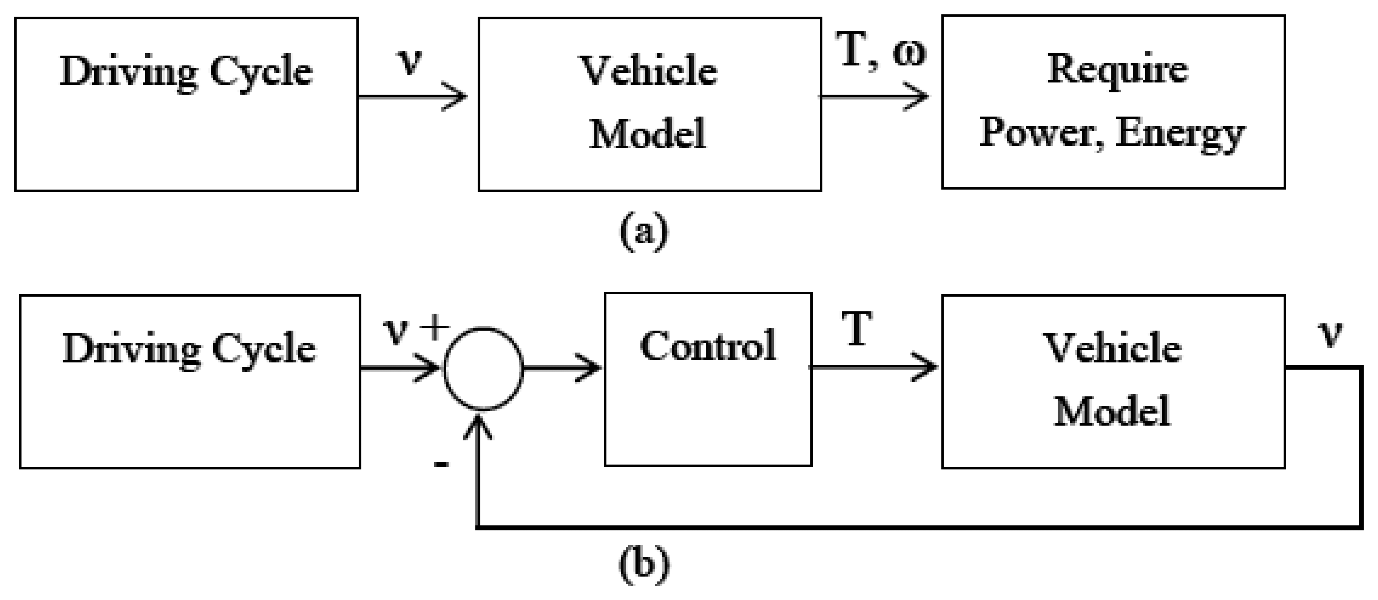
Many researchers have considered the application of formal optimization techniques to modeling: there is an excellent text on the subject by Guzzella and Sciarretta [6], and a recent article by Egardt et al. considered the subject in detail [7]. Broadly, there are two families of techniques: “forward-facing” modeling and “backwards-facing” modeling. Backward-facing model aims to drive a vehicle from velocity profile without a driver model. Simulation starts at speed reference form the driving cycle and determine required power and energy consumption. While forward-facing model utilises a driver model to obtain torque required for vehicle traction. Figure 1 shows a diagram of these modeling techniques.
The literature contains some discussion of the merits and disadvantages of the two [8,9]: “forward-facing” models can contain considerably more detail (in particular dynamics), but this has to be traded-off against the fact that quasi-static; “backwards-facing” models execute much more quickly. In some sources, the models which must be free from dynamics are expressed as algebraic equations [6]: if the driving cycle is fixed, it is often possible to express the energy consumed as a pure function of several parameters:
When there is more than one source of power, models of this can be extended to facilitate the design of optimal control trajectories and after some development implementable supervisory control laws. It is also possible to explore the sensitivity to parameter changes, giving an indication of which aspects of the design have the greatest influence on energy consumption and which areas of modeling require the greatest degree of accuracy.
The techniques in the literature provide methods of calculating sensitivity, but these only tell us about “first-order” sensitivities with very limited number of parameters, and do not give us insight into the cross-coupling between different parameters. In this paper, we develop formal techniques for exploring the cross-sensitivities between parameters and illustrate their application with a case study of a C-segment electric vehicle.
2. Mathematical Techniques for Sensitivity Analysis
2.1. First Order Sensitivity Analyses from the Literature
It is well-established in the literature [6] that when there is a fixed-drive cycle, optimizing an aspect of a system’s performance such as, say, energy consumption, it is possible to formulate a quasi-static model as a function of the key system parameters:
In other words:
If all we are interested in doing is working out these first-order sensitivities, then the mathematics in the literature is sufficient: it tells us which parameters are most important, which in turn tells us which parts of our system we should consider improving first and which parts of our models need to be the most accurate. However, it tells us nothing about the interactions between different parameters. In practice, we might find that improving the efficiency of a gearbox will mean that the efficiency of the electric machine connected to it becomes more significant. If we are developing a new vehicle, it is helpful to know whether we should be focusing all our efforts optimizing one thing, or whether we need to split our attention between several factors that will each in turn become important. We can address this by changing parameters and recalculating sensitivities for different possible scenarios, but it would be helpful to have a quicker, more intuitive way to understand things. We propose to address this through second-order calculus.
2.2. Change of Variables and Expression of Sensitivity via the Jacobian
The first step in our journey towards a second-order analysis is a change in variables. As before, let us assume we have a particular vehicle configuration described by the parameter set Φnom. Our first step is to perform a change of variables so we have an equation of the form:
To see the strength of this transformation, let us look again at Spi:
This expression will result in exactly the same values as the original expressions from the literature. This form is also easier to use when developing a second-order sensitivity analysis.
2.3. Expression of Second-Order Sensitivities via the Hessian with Illustrative Examples
We have seen that we can conveniently express (first-order) sensitivities through the Jacobian of our objective function. It is straightforward to find the second-order sensitivities from the Hessian of f̂(Φ̂):
This second-order sensitivity matrix gives us an indication of which sensitivities are cross-coupled. This will be examined by the following examples.
To start with, let us consider a problem where:
In this case the Jacobian is:
We can see here that Ê and therefore Ē is equally sensitive to each parameter. The Hessian is:
Which shows that the sensitivities are not cross-coupled: if we make a small change in p1, say, then the sensitivity to p2 will not change. Let us now consider another problem where:
Here, the Jacobian is:
As we might expect, this tells us that Ē will increase in response to a small relative change in p1 but a comparable change in p2 will cause a similarly-sized decrease. The Hessian is:
This yields some interesting results: we can see that if we start to increase p1 the sensitivity to p2 will increase and vice versa. We can also see that if we increase p2, the problem quickly becomes more sensitive to p2 itself; however, there is not a corresponding relationship for p1. We would see the potential power of this approach if we could imagine for a moment that p1 represents a vehicle’s powertrain efficiency and p2 represents its mass. We could conclude that if we were able to make the vehicle lighter, we would quickly find that the powertrain efficiency became a more significant factor in fine-tuning our design.
2.4. Expression of Second-Order Sensitivities in Original Unit Bases
The original definitions of sensitivity from the literature were stated in terms of the un-scaled “real-world parameters”, but we have expressed the second-order sensitivities in terms of normalized parameters. It may be more convenient to work with the original, untransformed units:
Note that with the untransformed variables, the second-order sensitivities are not given by the Hessian. To use the Hessian, we would need to apply appropriate scaling:
Here, the symbol “°” represents the Schur (element-wise) product.
In this section, we have developed techniques for applying formal second-order sensitivity analyses to our quasi-static vehicle models. These techniques will allow us to gain insight into the interdependencies of different parameters. The mathematics has been demonstrated using trivial examples, but a more elaborate case study based on a passenger car will be presented in the following section.
3. Case Study in Powertrain Optimization
In the previous section, we have introduced formal mathematics for sensitivity analysis; in this section we will apply these to a case study based on a popular real-world vehicle. Battery Electric Vehicles (BEVs) have now entered the mass consumer market. The Nissan LEAF a production C-segment vehicle is perhaps the best known. This section aims to present a simplified analytical BEV model and perform the first and second order sensitivity analysis. Vehicle parameters and powertrain components are based on publically available data [10] where possible, and are otherwise based on the authors’ assumptions: we have based our assumptions on the range performance data provided by the vehicle manufacturer [11]. In particular, we have aimed to reproduce the stated “combined” range of 175 km on the New European Driving Cycle (NEDC) with a 24 kWh battery.
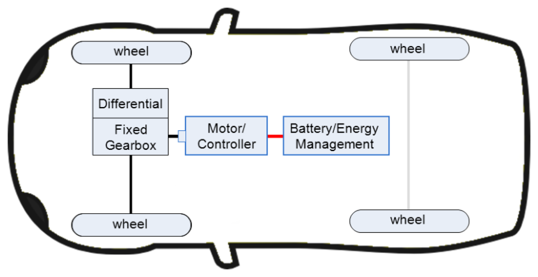
Figure 2 shows a schematic diagram of BEV powertrain of the Nissan LEAF. This vehicle is driven by a single 80 kW motor with a 7.9:1 constant ratio transmission at the front wheels. In backward facing simulation, to compute energy consumption, the calculations are started at the wheels. Driving cycle gives information of vehicle speed and losses due to environment are computed as functions of speed and acceleration then the required power at transmission, electric machine and battery is determined. Finally all losses are combined and the energy consumption of the vehicle is calculated.
For this paper, we have assumed that the nominal average fixed ratio transmission efficiency is 97%, the nominal average combine motor and inverter efficiency is 85% and we will associate this losses with motor losses, the battery average voltage (modeled as constant) is assumed to be 345 V, and the charge and discharge battery resistances are taken to be 216 × 10−3 ohm and 192 × 10−3 ohm.
We have also assumed that the vehicle is driving on a level surface, so we have ignored gradient effects. We have considered two driving cycles: the NEDC as specified in international testing standards [12], and a combined “real-world” cycle made from combinations of the well-known ARTEMIS cycles [13]. We have used a “combined” ARTEMIS cycle made from two cycles of the “urban” segment followed by two cycles of the “road” segment then one cycle of the “motorway” segment as we present in Figure 3. In the following subsections we will derive algebraic equations for describing the vehicle’s energy consumption, and then we will subject them to sensitivity analysis.
3.1. Vehicle Model and Energy Calculation
In this paper, we have considered the energy balance associated with the following elements: aerodynamic drag force, rolling friction force, inertial forces, transmission losses, losses in the motor, and losses in the battery. The reader is likely to be familiar with these, though a good text book can supply any deficit. Following [6], we will derive an energy equation based on the driving cycle:
Energy Balance Based on the Driving Cycle
Energy balance can be classified from the integral of summing force acting onto the vehicle and average speed on each of the driving cycle:
Note that for practical reasons, we will scale E so that it is expressed per unit distance rather than per unit time. (This is consistent with the way standards are presented and enables a better understanding of the results). In the following equations, xtotal is the driving distance (m).
The consumption due to aerodynamic losses, EAero, is given by:
The energy consumption from rolling resistance is given by:
The energy consumption from inertia is given by:
Motor losses are computed as:
Battery energy dissipation is calculated on both discharge and charge current:
3.2. Energy Consumption
Before we perform a sensitivity analysis, we will take a look at the predictions of energy consumption for our models and check that they are reasonable. Table 1 shows the energy consumption on each of the vehicle and powertrain components on both NEDC and combined Artemis driving cycles. Energy consumption presented on this table is in kWh (kilowatt-hour) per 100 km range based on the Equation (28) and using component sizes associated with the Nissan Leaf powertrain. Our assumption on the nominal regenerative braking efficiency is assumed to be 40%, but in this table the percentage of regenerative braking efficiency is selected differently to see the variation in energy consumption on each powertrain component. It is clear to see that the most consumed energy in both NEDC and combined Artemis are associated with the vehicle inertia. The other biggest losses are due to aerodynamic drag force and followed by rolling resistant losses. The regenerative energy recovery is simply calculated from the percentage of the energy from vehicle inertia. Battery losses are also included in this calculation as we present in the Equations (26) and (27). However, battery energy losses are very small and it is therefore safe to ignore these losses.
For the purposes of this paper, it is not critical that our model is exact, but we have demonstrated that it is at least reasonably representative. To see how sensitive our predictions are to parameter errors, we can use the results of the sections that follow. We can also see how improving any given component is likely to affect the overall energy consumption.
3.3. First-Order Sensitivity Analysis
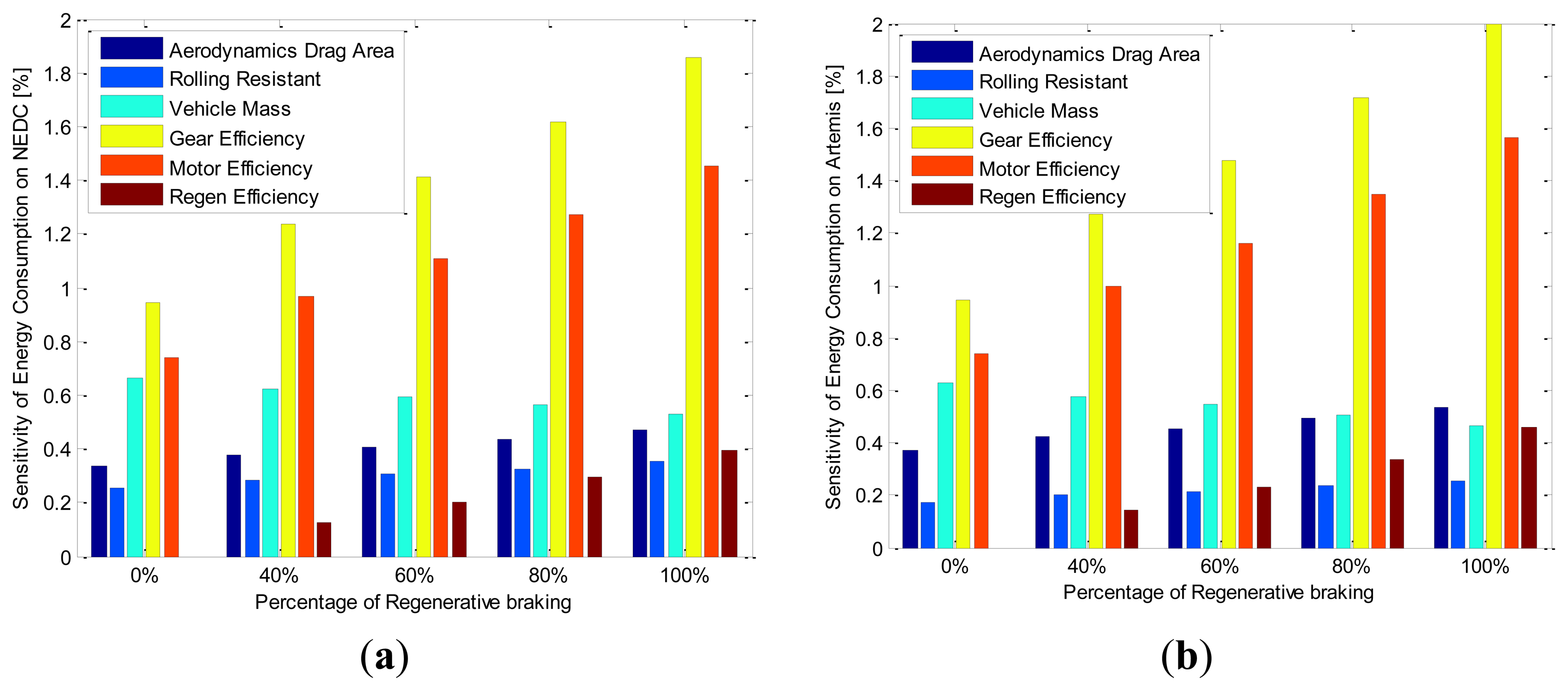
The techniques of Section 2 have been applied to the model and the results are shown in Figure 4. We can see that for both the NEDC and ARTEMIS cycles, the major parameter sensitivities are weight. As the regenerative braking efficiency improves, gear and motor efficiency become even more sensitive (note that changing the regenerative braking fraction from 40% to 100% results in a large relative change). Vehicle inertia sensitivity is reduced when the regenerative braking efficiency is improved; however, the relative change is much smaller compared with the sensitivity changes of gear and motor efficiencies. The aerodynamic and rolling resistance sensitivities are also increased as the regenerative braking energy efficiency is improved, but with a smaller relative change.
When comparing these two driving cycles, we can see a large difference in energy consumption, as illustrated in Table 1, but the relative change in sensitivities are comparable. We have observed some trends in the sensitivities for a single parameter, and to do so, we needed to produce several plots. In the following section, we will see whether a second-order analysis could have predicted this as well, and also that we can achieve similar results far more quickly and easily.
3.4. Second-Order Sensitivity Analysis
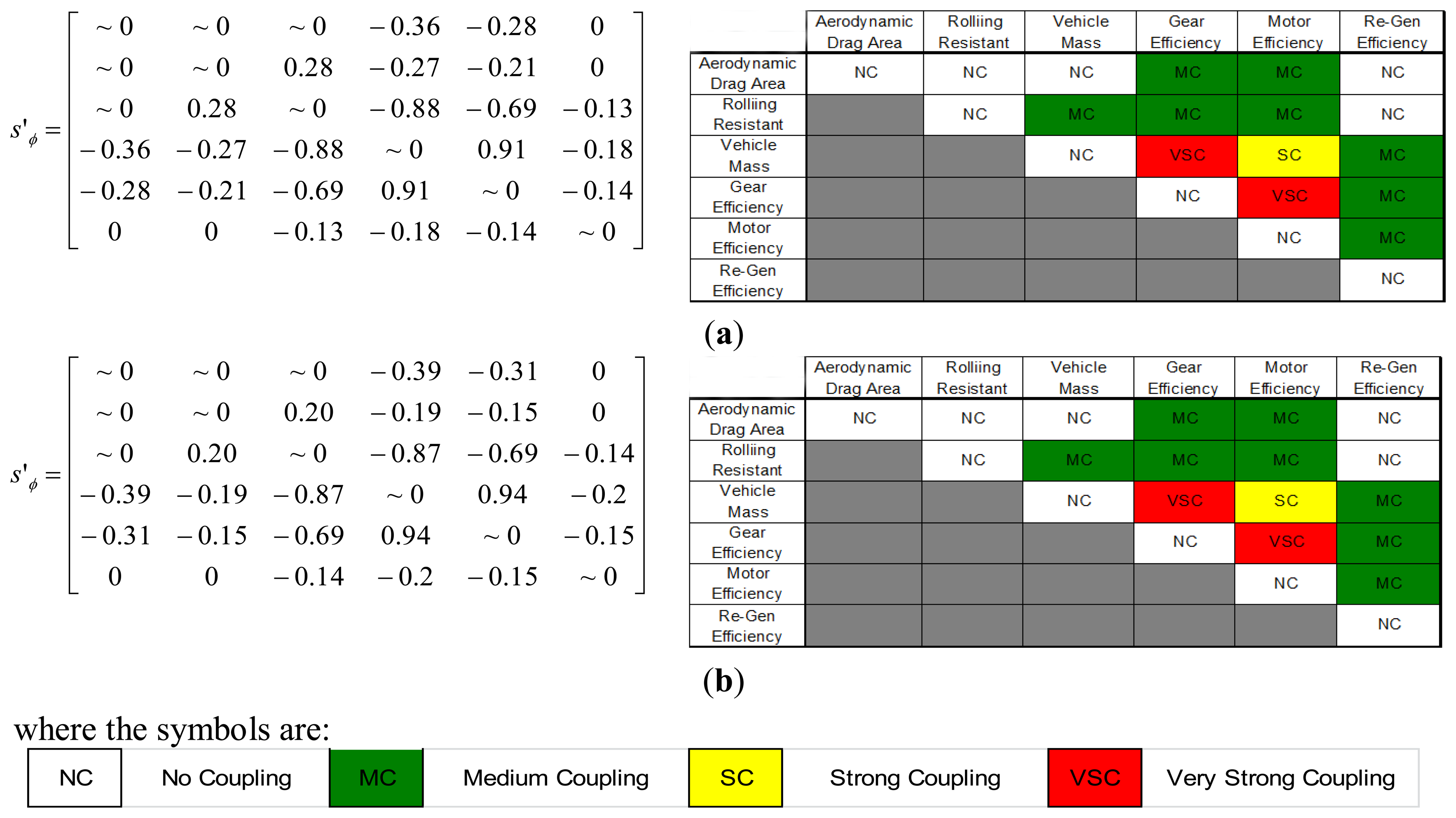
Figure 5 illustrates the results of second-order sensitivity analysis at the vehicle nominal points for NEDC and Artemis. Figure 5a shows the results for the NEDC in number values and text explanations and the same for Artemis cycle, as shown in Figure 5b.
It can be seen that the cross-coupling between the gear efficiency and the motor efficiency is very strong, as is the cross-coupling between gear efficiency and vehicle mass: the numerical values are close in magnitude to one. There is also strong cross-coupling between vehicle mass and motor efficiency. In fact, the gear and motor efficiency are also cross-coupled to every parameter. Cross-coupling between other parameters is smaller, and there are some cases where the cross-coupling is so small that it could be ignored. The same results are broadly true for both driving cycles. This relates well to the results shown in Figure 4: we see that that there is significant coupling between the sensitivities to regenerative braking efficiency, vehicle mass, gear efficiency and motor efficiency, but not much with the aerodynamic drag area and the rolling resistance.
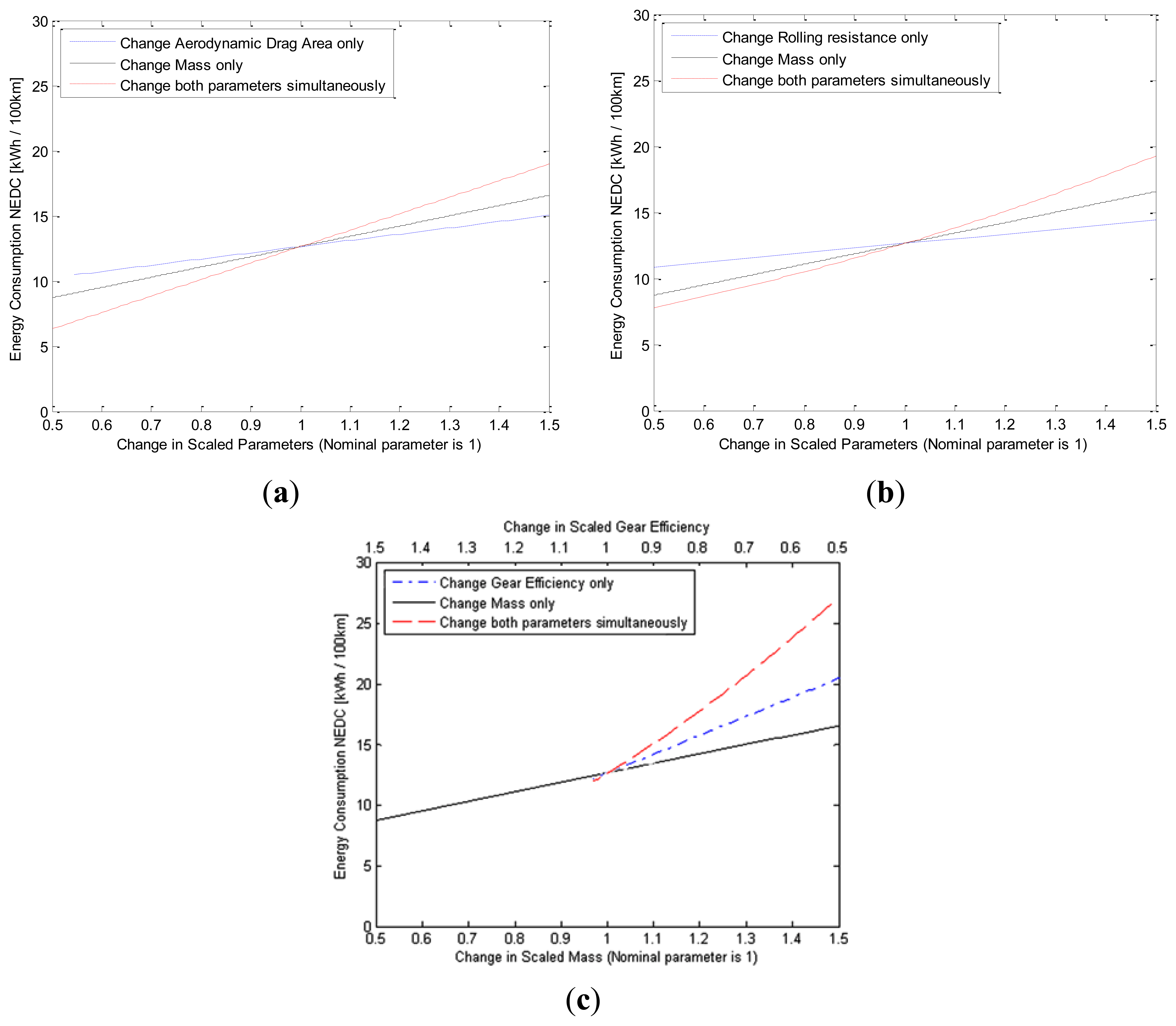
Figure 6 shows second order sensitivity results from selected parameters. In Figure 6a, energy consumption on NEDC of two parameters between aerodynamics and vehicle mass are presented. Black solid line illustrates change in vehicle mass only; blue dash-dot line shows change in aerodynamic area only. Red dash line shows changing in energy consumption while both parameters are changed simultaneously. We can see that there is no coupling between aerodynamic drag area and vehicle mass. As a result, when varying both parameters simultaneously, the impact on the energy consumption is linear due to the parameters being decoupled.
Figure 6b shows the coupling sensitivities for mass and rolling resistance and Figure 6c illustrates these sensitivities for mass and gear efficiency. The coupling between mass rolling resistance and mass gear efficiency are respectively medium and very strong as presented in Figure 5. When two parameters are varying simultaneously, the impact on the energy consumption changes non-linearly as shown in red-dash line. This is due to the coupling effect between the aforementioned parameters as presented in Section 3.4.
4. Discussion
The case study above has presented both first- and second-order sensitivity analyses. Compared to the literature, we have considered a large parameter set including “traditional parameters” such as drag area and mass, but also adding detailed characteristics of the powertrain such as the gearbox efficiency and the motor efficiency. For the legally-mandated NEDC and the more realistic ARTEMIS driving cycle, it has been shown that the greatest sensitivity is to the efficiency of the gearbox. This is particularly interesting because there are examples in the literature of attempts to reduce BEV energy consumption through the use of multiple transmission ratios to improve motor efficiency [14,15]. Typically, the use of multiple transmission ratios makes the gearbox efficiency worse. The sensitivity results of this paper suggest that in this particular case energy consumption is actually more sensitive to gearbox efficiency than motor efficiency, so we may want to keep the more-efficient single-speed transmission for the vehicle we have considered.
The first-order analysis has shown us which parameters have the greatest sensitivities, but the second-order analysis has shown how the parameters interact with each other. For example, we can see that there is very strong cross-coupling between the gearbox efficiency and the motor efficiency: this tells us that if we make the motor more efficient, the gearbox becomes (relatively) even more of a problem. If we are trying to produce optimal designs, we know that we need to be mindful of changes that will affect these parameters. We may need to make small changes together, for example.
Conversely, we saw that some other parameters are not strongly-coupled together. For those parameters, we do not need to take cross-coupling into account. As well as informing our design process, these sensitivities tell us about the accuracy of our results: if our model is very sensitive to a certain parameter, we need to be sure that we are accurate, because a small change would result in significantly misleading results.
For the vehicle manufacturer, insight into cross-coupling is useful since it can act as a guide as to which aspects of a vehicle configuration are particularly interconnected. A vehicle manufacturer will often want to use multi-objective optimization to address the trade-offs between design parameters. A second-order sensitivity analysis would aid in selecting the correct set of parameters for this type of optimization. A first-order analysis tells the manufacturer which components to improve first, but a second-order analysis gives an idea which components will be of significance next. In the case study, for example, we saw that drag area was only lightly coupled to drag gearbox efficiency, so we can work on one or the other in confidence, knowing that any gains will not be swamped by a new limiting factor. Conversely, we know that as we make the gearbox more efficient, the efficiency of the motor will become more of a relative problem. It would be interesting though probably not tractable to weight sensitivities with development costs as a tool to directing research investment.
The model we have used in this example is illustrative and some assumptions were made: we have assumed that the electric machine efficiency is a constant 85% efficiency both when motoring and generating; in practice, it varies. The model of regenerative braking is also simplified: some sources in the literature estimate an efficiency of around 50% [6], though this can depend greatly on the driving cycle and limitations imposed in the interest of good vehicle dynamics. We have also assumed a nominal transmission efficiency of 97%, which we feel is reasonable, but may not be perfect. Despite these limitations, we feel that our model is adequate for the purposes of this paper: sensitivity analysis shows which parameters will have the greatest effect on the results, if inaccuracies in our model are significant, sensitivity analysis will highlight this.
5. Conclusions
This paper has presented an extended technique for analyzing parameter sensitivities in modern road vehicles. The new techniques consider first-order and second-order effects, showing both the effects on individual parameters and also the cross-coupling between different parameter sensitivities. This method is quick and intuitive, and will help a vehicle designer quickly gain extra insights and identify cross-coupled parameters. The techniques have been demonstrated on an energy-minimization problem for a C-segment BEV. The parameter set considered was larger than that typically encountered in the literature, and highlighted the sensitivity of the result to the powertrain efficiency.
The work to date has considered only a single topology in a theoretical context, and it would be interesting to conduct further work determining how useful second-order analyses are in practice. Second-order analysis could potentially inform research and development work, aiding engineers to understand how “limiting factors” interact and giving insight into the technical challenges that will arise once today’s problems have been addressed. However, to be certain of benefits, it would be worth evaluating the techniques in the context of a development project and determining whether the theory translates into useful practice. The authors plan to test these techniques with different powertrain topologies.
Acknowledgments
Pongpun Othaganont thanks the Ministry of Science & Technology, Thailand, for the funding that supported this work.
Conflicts of Interest
The authors declare no conflict of interest.
References
- Gao, D.W.; Mi, C.; Emadi, A. Modeling and simulation of electric and hybrid vehicles. Proc. IEEE 2007, 95, 729–745. [Google Scholar]
- Bashash, S.; Moura, S.J.; Forman, J.C.; Fathy, H.K. Plug-in hybrid electric vehicle charge pattern optimization for energy cost and battery longevity. J. Power Sources 2011, 196, 541–549. [Google Scholar]
- Auger, D.J.; Groff, M.F.; Mohan, G.; Longo, S.; Assadian, F. The impact of battery ageing on an electric vehicle powertrain optimisation. Proceedings of the 8th Conference on Sustainable Development of Energy, Water and Environment Systems, Dubrovnik, Croatia, 22–27 September 2013.
- Ribau, J.P.; Silva, J.M.S.; Silva, C.M. Multi-objective optimization of fuel cell hybrid vehicle powertrain design cost and energy. Proceedings of 11th International Conference on Engines & Vehicles, Capri, Napoli, Italy, 16–19 September 2013.
- Ribau, J.; Viegas, R.; Angelino, A.; Moutinho, A.; Silva, C. A new offline optimization approach for designing a fuel cell hybrid bus. Transp. Res. C Emerg. Technol. 2014, 42, 14–27. [Google Scholar]
- Guzzella, L.; Sciarretta, A. Vehicle Propulsion Systems, Introduction to Modeling and Optimization; Springer: Berlin/Heidelberg, Germany, 2005. [Google Scholar]
- Egardt, B.; Murgovski, N.; Pourabdollah, M.; Johannesson, L. Electromobility studies based on convex optimization. IEEE Control Syst. 2014, 34. [Google Scholar] [CrossRef]
- Wipke, K.B.; Cuddy, M.R.; Burch, S.D. ADVISOR 2.1: A user-friendly advanced powertrain simulation using a combined backward/forward approach. Veh. Technol. IEEE Trans. 1999, 48, 1751–1761. [Google Scholar]
- Mohan, G.; Assadian, F.; Longo, S. Comparative analysis of forward-facing models vs. backward-facing models in powertrain component sizing. proceedings of IET Hybrid and Electric Vehicles Conference (HEVC 2013), London, UK, 6–7 November 2013.
- Hayes, J.G.; de Oliveira, R.P.R.; Vaughan, S.; Egan, M.G. Simplified electric vehicle power train models and range estimation. Proceedings of Vehicle Power and Propulsion Conference (VPPC), Chicago, IL, USA, 6–9 September 2011; pp. 1–5.
- Nissan. Available online: http://www.nissan.co.uk (accessed on 9 April 2014).
- United Nations. Concerning the Adoption of Uniform Technical Prescriptions for Wheeled Vehicles, Equipent and Parts which can be Fitted and/or be Used on Wheeled Vehicle and the Conditions for Reciprocal Recognition of Approvals Granted on the Basic of these Prescriptions; United Nations: Herndon, VA, USA, 2005. [Google Scholar]
- André, M. The ARTEMIS European driving cycles for measuring car pollutant emissions. Sci. Total Environ. 2004, 334, 73–84. [Google Scholar]
- Othaganont, P.; Assadian, F.; Auger, D. Cycle-based optimisation of multi-speed transmission for battery electric vehicles. Proceedings of Future Powertrain Conference, National Motorcycle Museum, Solihull, UK, 19–20 February 2014.
- Stubbs, B.; Ceng, P. eDCT: 4 Speed Seamless-Shift Technology For Electric Vehicles. Proceedings of the IET Hybrid and Electric Vehicles Conference (HEVC 2013), London, UK, 6–7 November 2013.


| Energy (kWh·100 km−1) | NEDC 0% regen | NEDC 40% regen | NEDC 50% regen | NEDC 80% regen | NEDC 100% regen |
|---|---|---|---|---|---|
| Aerodynamics | 4.03 | 4.03 | 4.03 | 4.03 | 4.03 |
| Rolling Resistance | 3.05 | 3.05 | 3.05 | 3.05 | 3.05 |
| Vehicle Mass | 4.95 | 4.95 | 4.95 | 4.95 | 4.95 |
| Regenerative Recovery | 0.00 | −1.98 | −2.47 | −3.96 | −4.95 |
| Transmission Loss | 0.36 | 0.42 | 0.44 | 0.48 | 0.51 |
| Motor Loss | 1.86 | 2.16 | 2.24 | 2.47 | 2.62 |
| Battery Discharge Loss | Negligible | ||||
| Battery Charge Loss | Negligible | ||||
| Total Energy (kWh·100 km−1) | 14.25 | 12.63 | 12.23 | 11.02 | 10.21 |
| Energy (kWh·100 km−1) | Artemis 0% regen | Artemis 40% regen | Artemis 50% regen | Artemis 80% regen | Artemis 100% regen |
| Aerodynamics | 6.42 | 6.42 | 6.42 | 6.42 | 6.42 |
| Rolling Resistance | 3.05 | 3.05 | 3.05 | 3.05 | 3.05 |
| Vehicle Mass | 7.91 | 7.91 | 7.91 | 7.91 | 7.91 |
| Regenerative Recovery | 0.00 | −2.37 | −3.95 | −6.33 | −7.91 |
| Transmission Loss | 0.52 | 0.59 | 0.64 | 0.71 | 0.76 |
| Motor Loss | 2.68 | 3.05 | 3.30 | 3.66 | 3.91 |
| Battery Discharge Loss | Negligible | ||||
| Battery Charge Loss | Negligible | ||||
| Total Energy (kWh·100 km−1) | 20.58 | 18.64 | 17.35 | 15.42 | 14.13 |
© 2014 by the authors; licensee MDPI, Basel, Switzerland. This article is an open access article distributed under the terms and conditions of the Creative Commons Attribution license ( http://creativecommons.org/licenses/by/3.0/).
Share and Cite
Othaganont, P.; Assadian, F.; Auger, D. Sensitivity Analyses for Cross-Coupled Parameters in Automotive Powertrain Optimization. Energies 2014, 7, 3733-3747. https://doi.org/10.3390/en7063733
Othaganont P, Assadian F, Auger D. Sensitivity Analyses for Cross-Coupled Parameters in Automotive Powertrain Optimization. Energies. 2014; 7(6):3733-3747. https://doi.org/10.3390/en7063733
Chicago/Turabian StyleOthaganont, Pongpun, Francis Assadian, and Daniel Auger. 2014. "Sensitivity Analyses for Cross-Coupled Parameters in Automotive Powertrain Optimization" Energies 7, no. 6: 3733-3747. https://doi.org/10.3390/en7063733