Refined Diebold-Mariano Test Methods for the Evaluation of Wind Power Forecasting Models

Abstract

The scientific evaluation methodology for the forecast accuracy of wind power forecasting models is an important issue in the domain of wind power forecasting. However, traditional forecast evaluation criteria, such as Mean Squared Error (MSE) and Mean Absolute Error (MAE), have limitations in application to some degree. In this paper, a modern evaluation criterion, the Diebold-Mariano (DM) test, is introduced. The DM test can discriminate the significant differences of forecasting accuracy between different models based on the scheme of quantitative analysis. Furthermore, the augmented DM test with rolling windows approach is proposed to give a more strict forecasting evaluation. By extending the loss function to an asymmetric structure, the asymmetric DM test is proposed. Case study indicates that the evaluation criteria based on DM test can relieve the influence of random sample disturbance. Moreover, the proposed augmented DM test can provide more evidence when the cost of changing models is expensive, and the proposed asymmetric DM test can add in the asymmetric factor, and provide practical evaluation of wind power forecasting models. It is concluded that the two refined DM tests can provide reference to the comprehensive evaluation for wind power forecasting models.

1. Introduction

Global power systems are involving more novel sustainable clean energy sources to lead clean operation and sustainable living [1]. Specifically, wind energy is one of the fastest growing energy sources [2,3,4]. In China, the total installed wind power capacity is expected to be 30 GW by 2020 [5]. Due to the volatility and intermittency of wind, the generation of wind power in wind farms usually varies over a wide range, making it difficult to accurately set up a dispatch plan [6]. As a result, a number of methods have been introduced for wind power forecasting [7,8]. Generally, physical models [9], statistical models [10,11,12,13,14,15] and hybrid approaches [16] are the three main methodologies used in wind power forecasting. References [10,11] employ the Auto-Regressive Moving Average (ARMA) model to predict wind power and obtain effective forecasting results. However, the classical time series model might have shortcomings in the break point of the wind power time series; reference [12] used Generalized Autoregressive Conditional Heteroskedasticity (GARCH) models to take into account the volatility of wind power; reference [13] used wavelet, time series and Artificial Neural Network (ANN) methods for wind speed forecasting, In addition, spatial models [14], and Kalman filter techniques [15] are also applied in wind speed forecasting as effective statistical methods. Based on the application of hybrid approaches, reference [16] provided wind power forecasting by the flexible combination of dynamic models.

A number of practical wind power forecasting systems serving in Chinese dispatch departments can provide several kinds of paralleling forecasting methods for the reference of the dispatcher. Due to the volatility of wind power, it is helpful to figure out an outstanding model from the competing forecasting models. Consequently, model evaluation of the forecasting accuracy is an interesting and challenging topic in this field. In practice, the traditional statistical evaluation indices, such as Mean Squared Error (MSE), Mean Absolute Error (MAE) and the variety of others are widely employed to evaluate forecasting results and make forecasting comparisons. Though these traditional statistical evaluation indices are simple and easily understood, they have limitations in some cases. On the one hand, considering the ubiquity of sample randomness, forecasting results given by different forecasting models can be interfered by stochastic difference. When the influence of stochastic difference is strong enough, the traditional indices can even give misleading comparison results in the most unfavorable cases [17]. On the other hand, the traditional indices cannot give quantitative thresholds for comparison of forecasting with different wind power forecasting models; they can only provide qualitative analysis. Compared to the study on forecasting methods, the study on the forecasting evaluation [18,19,20] is far from sufficiently well covered in the literature. In this paper, a modern evaluation criterion, the Diebold-Mariano (DM) test [21], is induced to quantitatively evaluate the different wind power forecasting models, and the DM test is further refined in two ways to enhance the efficiency of the evaluation.

The remainder of the paper is organized as follows: Section 2 first reports the limitations of the traditional evaluation criteria. Then the DM test is introduced and two types of refined DM test, the augmented DM test and the asymmetric DM test, are proposed in this part. In the case study of Section 3, the DM test is first used to evaluate the forecasting performance of several wind power forecasting models. Furthermore, the rolling sample technology is employed in the augmented DM test to enhance the results, and the asymmetric DM test is provided to give a more practical wind power forecasting evaluation. Section 4 provides a discussion about the DM test, and Section 5 presents the conclusions.

2. The Evaluation Criteria for Wind Power Forecasting Models

2.1. Traditional Evaluation Criteria and Their Limitations

Traditionally, several statistical indices are usually used as the evaluation criteria for wind power forecasting models. Table 1 summarizes six indices and their specifications.

Table 1. Traditional evaluation criteria.

Index	Abbreviator	Specification
Mean Squared Error	MSE
Root Mean Squared Error	RMSE
Mean Absolute Error	MAE
Mean Absolute Percentage Error(%)	MAPE
Maximum Error	ME	ME = max (|yt − ŷt|)
Theil Inequality Coefficient	TIC

Table 1. Traditional evaluation criteria.

Index	Abbreviator	Specification
Mean Squared Error	MSE
Root Mean Squared Error	RMSE
Mean Absolute Error	MAE
Mean Absolute Percentage Error(%)	MAPE
Maximum Error	ME	ME = max (|yt − ŷt|)
Theil Inequality Coefficient	TIC

Note that y_t is the actual wind power data; ŷ_t is the forecasting value; T is the sample size; and h is the forecast step size.

In practice, MSE and MAE are the most popular evaluation criteria. On behalf of the traditional criteria, MSE is used to analyze the limitations of traditional evaluation criteria in this paper. In the following part, a forecasting comparison is made between two models, say, model A and model B.

After calculating the MSE of the forecasting result, if the MSE difference between model A and model B is small, it is in fact difficult to decide whether the result is due to chance or decisive. In fact, the answer cannot be simply concluded from the MSE value. If a small MSE difference is approved and the model with smaller MSE is accepted, we may then possibly reject a factually good parallel model because the difference may be generated stochastically.

As a result, whether the difference of forecasting performances is significant in the statistic view cannot be efficiently judged by the traditional evaluation criteria. To solve this problem, a modern statistic evaluation method, the Diebold-Mariano (DM) test, which can offer a quantitative method to evaluate the forecast accuracy of wind power forecasting models, is proposed in this paper.

2.2. Diebold-Mariano Test

The classical DM test was originally proposed by Diebold and Mariano [17,21]. The routine of the classical version of DM test is as follows:

Let {y_t} denote the actual data series. Let denote the i^th competing h-step forecasting series.

Supposing the forecasting errors from the i^th competing models are (i = 1, 2, 3,…m). where m is the number of the forecasting models. The h-step forecasting errors is:

(1)

The accuracy of each forecast is measured by the loss function:

(2)

In this paper, h is set to be 1, and the superscript h is omitted in the following context. There are lots of loss functions, and the most popular and usually adopted loss functions in power systems are the squared-error loss function and the absolute-error loss function.

Squared-error loss function:

(3)

Absolute-error loss function:

(4)

The squared-error loss and the absolute-error loss are both symmetric around the origin point. Furthermore, larger errors are penalized more severely by the squared-error loss one.

To determine whether one forecasting model (say, the first model, model A) predicts more accurately than another (say, the second model, model B), we may test the equal accuracy hypothesis. The null hypothesis is given as:

H₀ : E[L(e_1,t)] = E[L(e_2,t)]

The alternative hypothesis that one is better than the other is given as:

H₁ : E[L(e_1,t)] ≠ E[L(e_2,t)]

The Diebold-Mariano test is based on the loss differentials d_t:

d_t = L(e_1,t − L(e_2,t)

(5)

Equivalently, the null hypothesis of equal predictive accuracy is shown as H₀: E[d_t] = 0. Then, let the sample mean loss differential, d, be:

(6)

Note that the DM test statistic is:

(7)

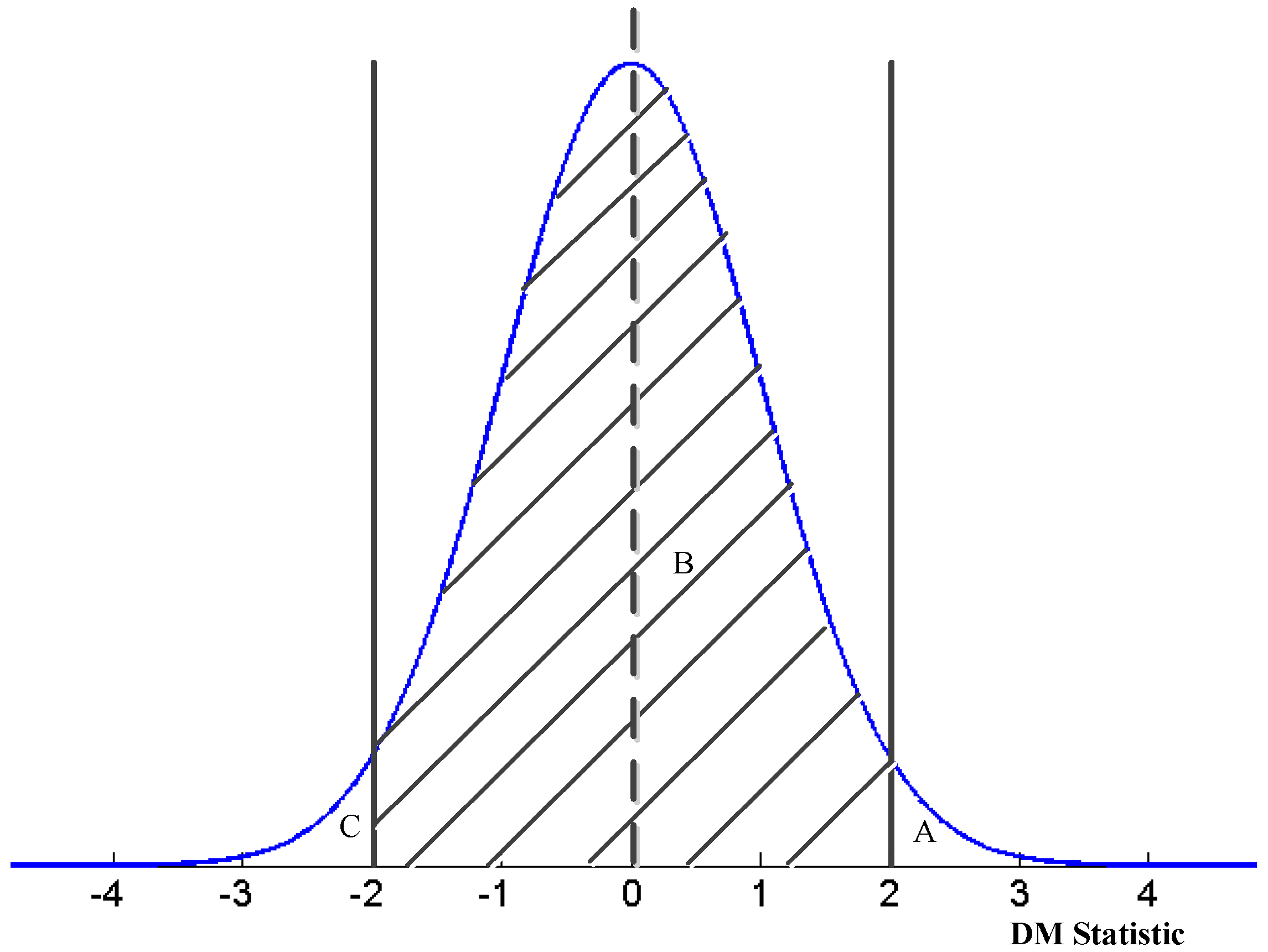
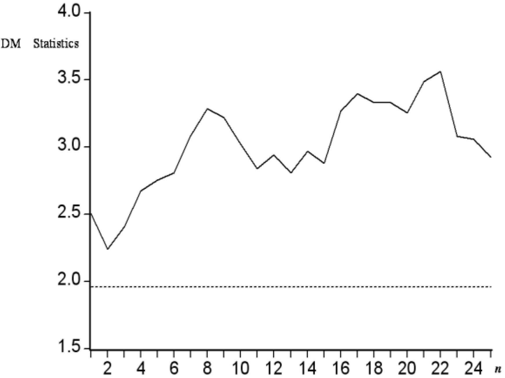
where is a consistent estimator of the asymptotic variance of . Note that the variance is used in the statistic because the sample of loss differentials d_t are serially correlated for h > 1. Since the DM statistics converge to a normal distribution, we can reject the null hypothesis at the 5% level if |DM| > 1.96; this condition corresponds to the zone A and zone C in Figure 1. Otherwise, if |DM| ≤ 1.96, we cannot reject the null hypothesis H₀, and this case corresponds to zone B in Figure 1.

Figure 1. The normal distribution.

Figure 1. The normal distribution.

2.3. Augmented DM Test

With the help of the DM test, the interference by sample stochastic difference can be revealed, such that the better forecasting model can be figured out statistically. However, since the cost of changing the in-service forecasting model may be expensive in some special cases, evaluation judgments should be given more carefully, and it will be beneficial if more strong evidence can be found. The augmented DM test is proposed in this part to provide more evidence for model evaluation. The augmented DM test can provide more refined studies based on a sequence of DM test results by evolving a rolling sample approach [22]. The specification of this approach is as follows:

Firstly, a dataset window covering part of the total sample is selected, and two forecasting result series can be obtained by two types of wind power forecasting models based on this subsample. Then, based on the calculation of the forecasting error series e_1,t, e_2,t, respectively, the DM test is employed to evaluate forecasting accuracy.

Secondly, by adding in the next p data and removing the first p data in the above mentioned dataset, a new subsample can be obtained with the same length. Under this condition, the two competing wind power forecasting models are used again based on this new window. Once again, the DM test based on the new subsample is employed to provide a new evaluation.

Consequently, the time varying window keeps on rolling, and the new wind power forecasting models are re-estimated by carrying out DM tests based on new sub-samples. The retest work does not stop until the rolling windows cover the pre-established whole sample space.

Finally, based on the augmented DM test method, the DM statistics based on all of the sub-samples are performed. If the H₀ hypothesis of DM test is rejected in every sub-sample, the enhanced H₀ hypothesis of augmented DM test will be rejected, and a better model is reported. Otherwise, even if only one H₀ hypothesis is not rejected in one subsample, then the H₀ hypothesis of augmented DM test cannot be rejected.

It is clear that the augmented DM test has more rigid requirements than the DM test. During the process of the augmented DM test, if at least one H₀ hypothesis of a sub-sample DM test cannot be rejected, then the augmented DM test will report the failure of selecting a better model. Thus dispatchers may not tend to change the in-service model if model changing is expensive. On the other hand, if all of the H₀ hypotheses of sub-sample DM tests are rejected, that is to say, the rigid requirements of the augmented DM test are satisfied, then the strong evidence that one forecasting model is better by far is confirmed, and the confidence of judging the better model is greatly increased.

2.4. Asymmetric DM Test

Though reference [20] recognizes that the extensive loss function could be imposed considering asymmetric loss, in practice, the most popular loss functions are symmetric loss function, such as squared-error loss function and absolute-error loss function.

For wind power forecasting, the cost of seriously overestimating the wind power is not equal to the cost of seriously underestimating it. For example, in view of the stability, if the forecasting error e_t is positive and big enough, that is to say, the actual wind power is far larger than the forecast given by the wind power forecasting model, the cost is higher than the case when e_t is negative.

Limited to symmetric structure, neither the squared-error loss, nor the absolute-error loss can be an adequate description of the forecasting environment. In this case, the asymmetric loss function may help evaluate the forecasting accuracy. As a result, to make it practical, the DM tests based on the asymmetric loss functions, which are named asymmetric DM tests, are proposed in this paper.

Two types of asymmetric loss functions are employed as follows:

Type I asymmetric loss function is:

(8)

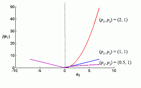
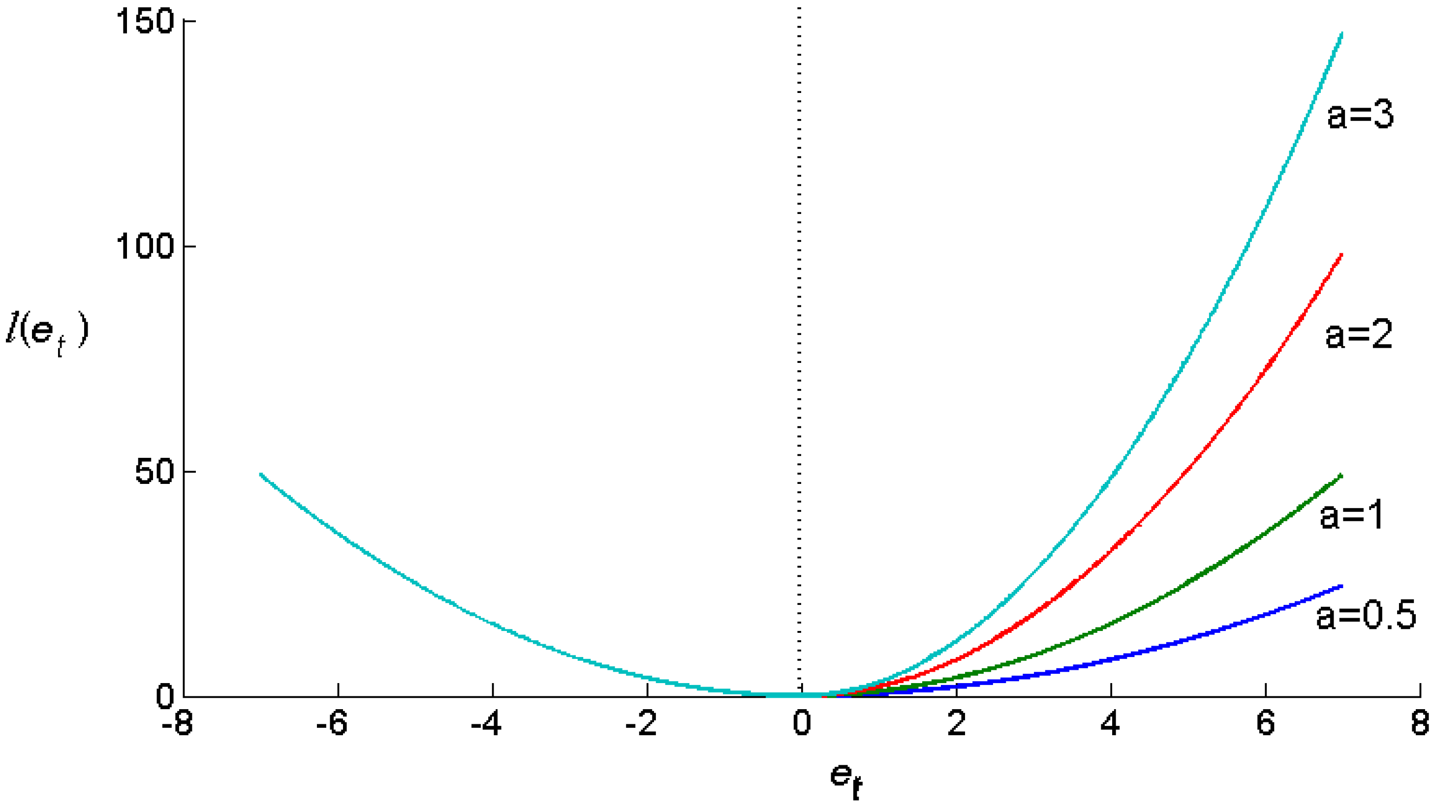
where , p is a positive integer valued power parameter; a is the asymmetric index parameter. If a = 1, the type I asymmetric loss function is reduced to a symmetric loss function. Moreover, if a = 1 and p = 2, the loss function is reduced to a squared-error loss function.

Type II asymmetric loss function is:

(9)

where , p₁ and p₂ are positive integer valued asymmetric power parameters. If p₁ = p₂ = 2, the Type II asymmetric loss function is reduced to a squared-error loss function. Otherwise, if p₁ = p₂ = 1, the loss function is reduced to an absolute-error loss function.

The l_aI,i in Type I asymmetric loss functions with the asymmetric parameter a = 0.5, a = 1, a = 2, or a = 3, respectively, are drawn in Figure 2.

Figure 2. l_aI in Type I Asymmetric Loss Function with Different Parameters (p = 2).

Figure 2. l_aI in Type I Asymmetric Loss Function with Different Parameters (p = 2).

The l_aII,i in Type II asymmetric loss functions with the power parameter pairs (p₁, p₂) = (2, 1), (p₁, p₂) = (1, 1), (p₁, p₂) = (0.5, 1), respectively, are shown in Figure 3.

Figure 3. l_aII in Type II Asymmetric Loss Function with Different Parameters.

Figure 3. l_aII in Type II Asymmetric Loss Function with Different Parameters.

With the help of the asymmetric loss function, the difference between the cost of overestimating and underestimating can be measured separately and reasonably.

3. Case Study and Results

3.1. Data

The historical wind power data from a coastal wind farm group in Jiangsu Province is used to examine the presented wind power forecasting models. As a province with rich coastal wind resources in East China, the wind power data from Jiangsu Province can be representative of a typical wind power pattern in China. The sample consists of 5 day wind power data recorded in spring, 2012. The wind power data is obtained every 10 min. With 144 datapoints each day, the 5 day overall data sample contains 720 datapoints. The 10 min wind power forecasting of the following 4 h is studied using three wind power forecasting models, and the refined DM tests are carried out for the evaluation of the different wind power forecasting models.

3.2. Forecasting Models

Three popular wind power forecasting models, the GARCH model [22,23], TAR model [24] and ARMA model [19], are used for evaluation. The performance of these three models are validated by comparison to the actual data, and then examined based on the proposed modern evaluation method.

The software Eviews is firstly employed in parameter estimation and wind power forecasting with the different forecasting models. Furthermore, the software R is used to carry out the DM test and the refined DM tests. First of all, the exponential trend, T_trend, is eliminated from the initial daily data series, and the time series after adjustment is noted as I_ad. Then I_ad are modelled by the above- mentioned three models. The three models are estimated by conditional maximum likelihood estimation (CMLE) [25,26]. At the same time, the Marquardt algorithm, a well-known modified version of the Gauss-Newton algorithm, is used to control the iteration process.

3.3. Forecasting Performance

After eliminating the exponential trend, the wind power forecasting formation is expressed as:

Ŷ = T_trend × Î_ad

(10)

where, T_trend is the exponential trend of the initial daily data series; Î_ad is modelled by the GARCH, TAR and ARMA models, respectively. Based on the three forecasting models above, 10 min forecasting results of wind power for the following 4 h are obtained. Two traditional statistical indices, MSE and MAE, are reported in Table 2.

Table 2. Comparison of forecasting performance.

Models	MAE	MSE
Model A:GARCH	1.916871	4.315878
Model B:TAR	2.571685	10.08665
Model C:ARMA	2.614892	10.02256

Table 2. Comparison of forecasting performance.

Models	MAE	MSE
Model A:GARCH	1.916871	4.315878
Model B:TAR	2.571685	10.08665
Model C:ARMA	2.614892	10.02256

From Table 2, we can find that the forecasting results of model A looks intuitively better than the other two models by MAE or MSE. However, the MSE difference between model B and model C is difficult to distinguish. MSE is invalid to decide whether the difference is due to chance. It is necessary to employ the DM test to evaluate the forecast accuracy, and differentiate the forecasting performance of model B and model C.

3.4. Forecasting Evaluation Based on DM Test

In this part, the forecasting performance of the three models is compared by the DM test. Using the classical version of the DM test demonstrated in Section 2, the forecasting comparison of every two forecasting models is summarized in Table 3, respectively. The zero hypothesis, H₀: E[L(e_1,t)] = E[L(e_2,t)], means that the observed differences between the performance of two forecasting models is not significant, while the alternative hypothesis, H₁: E[L(e_1,t)] ≠ E[L(e_2,t)], means that the observed differences between the performance of two forecasting models is significant.

Table 3. The DM test.

	DM test based on Model A and Model B	DM test based on Model B and Model C	DM test based on Model C and Model A
DM-AE	−1.5168	−0.0852	1.7401
p-Value_DM-AE	0.1429	0.9328	0.0952
DM-SE	−2.3647	0.0213	2.5044
p-Value_DM-SE	0.026861	0.9832	0.0198

Note: DM-AE denotes the DM test statistic based on absolute-error loss; DM-SE denotes the DM test statistic based on squared-error loss.

Table 3. The DM test.

	DM test based on Model A and Model B	DM test based on Model B and Model C	DM test based on Model C and Model A
DM-AE	−1.5168	−0.0852	1.7401
p-Value_DM-AE	0.1429	0.9328	0.0952
DM-SE	−2.3647	0.0213	2.5044
p-Value_DM-SE	0.026861	0.9832	0.0198

Note: DM-AE denotes the DM test statistic based on absolute-error loss; DM-SE denotes the DM test statistic based on squared-error loss.

From Table 3, the conclusions of the comparison of model A and model B can be drawn:

(1)

According to the DM test based on the absolute-error loss, since the absolute value of DM-AE is 1.5168, that is, less than 1.96, the zero hypothesis cannot be rejected at the 5% level of significance, that is to say, the observed difference between the forecasting performance of model A and model B is not significant and might me due to stochastic interference.

(2)

According to the DM test based on the squared-error loss, since the absolute value of DM-SE = 2.3647 > 1.96, the zero hypothesis is rejected at the 5% level of significance, that is to say, the observed differences are significant and the forecasting accuracy of model A is better than that of model B.

Similarly, according to the forecasting comparison of model B and model C in Table 3, both the DM test by absolute-error loss and the DM test by squared-error loss evaluate that the forecasting performance of model B and model C is not significant and might due to stochastic interference.

Finally, the forecasting comparison of model C and model A is summarized in Table 3. In Table 3, the zero hypotheses of the DM test based on the two types of loss function are rejected at the 10% level of significance. However, at the 5% level of significance, DM-AE = 1.7401 < 1.96, the DM test by absolute-error loss shows that the forecasting performance of model C and model A is not significant and might due to stochastic interference.

3.5. Forecasting Evaluation Based on Augmented DM Test

In some special cases, the cost of changing the in-service wind power forecasting model is great. To give a more strict evaluation, the augmented DM test is employed in the case study. Overall, the retest work generates 24 DM statistics based on squared-error loss for the augmented forecasting comparison of model C and model A. The dynamic structure details of the DM statistics are analyzed by the augmented DM statistics line, as illustrated in Figure 4.

Figure 4. Statistic line of the augmented DM test between model A and model C.

Figure 4. Statistic line of the augmented DM test between model A and model C.

In Figure 4, the curve corresponds to a series of DM statistics in the sub-sample windows. It is easy to observe that the augmented DM statistics curve varies beyond 1.96, the threshold value. According to Figure 4, it is clear that the result of DM test varies stably, demonstrating significance of forecasting difference over the different sample space. Even in a guarded view, the forecasting performance of model A is better than model C. At this time, enough confidence is obtained for concluding the better model.

3.6. Forecasting Evaluation Based on Asymmetric DM Test

Considering the characteristics of wind power forecasting discussed in Section 2, the negative half branch of the loss function should be flatter than the positive half branch. Two types of asymmetric loss functions are employed in the asymmetric DM test. With a = 2, p = 2, the l_aI,i in Equation (8) is rewritten as:

(11)

With the p₁ = 2, p₂ = 1, the l_aII,i in Equation (9) is rewritten as:

(12)

With the two types of asymmetric DM test, the forecasting comparison of every two forecasting models is summarized in Table 4, respectively.

Note that the Type I asymmetric DM statistic is expressed as DM-aI for short. Similarly, the Type II asymmetric DM statistic is expressed as DM-aII for short. The zero hypothesis, H₀: E[L(e_1,t)] = E[L(e_2,t)], means that the observed differences between the performance of two forecasting models is not significant, while the alternative hypothesis, H₁: E[L(e_1,t)] ≠ E[L(e_2,t)], means that the observed differences between the performance of two forecasting models is significant.

Table 4. Asymmetric DM test.

	Comparison of model A and model B	Comparison of model B and model C	Comparison of model C and model A
DM-aI	−2.2429	−0.7747	3.1649
p-Value_ DM-aI	0.02966	0.4424	0.002721
DM-aII	−1.711	−0.3481	2.2932
p-Value_ DM-aII	0.09367	0.7293	0.02635

Table 4. Asymmetric DM test.

	Comparison of model A and model B	Comparison of model B and model C	Comparison of model C and model A
DM-aI	−2.2429	−0.7747	3.1649
p-Value_ DM-aI	0.02966	0.4424	0.002721
DM-aII	−1.711	−0.3481	2.2932
p-Value_ DM-aII	0.09367	0.7293	0.02635

From Table 4, the following conclusions can be safely drawn:

(1)

Different loss functions will induce different DM test results. The forecasting accuracy of model A and model C is equally matched by DM-AE, as shown in Table 3. However, the forecasting accuracy of the two models is significantly different by the DM-aI test and DM-aII test. Consequently, a reasonable loss function will help to choose the better model.

(2)

The asymmetric loss can penalize large positive forecasting errors, e_t. If the positive forecasting errors are large enough, the zero hypothesis of the DM test based on asymmetric loss tends to be rejected. Model C has several large positive forecasting errors, while model A is outstanding in the view of large positive forecasting errors, so model C is worse than model A by the asymmetric DM test based on asymmetric loss.

4. Discussion

The scientific evaluation of the forecast accuracy of wind power forecasting models is an important issue in the wind power forecasting domain. Compared to the traditional evaluation indices, the DM test plays an important theoretical role, and it has been successfully applied in many occasions. However, the standard version of the DM test cannot practically answer all of the questions for the evaluation of wind power forecasting models. For example, as mentioned in Section 2.3, when the cost of changing the in-service wind power forecasting model in the dispatch system is high, a single round of DM tests might be arbitrary. By employing the proposed augmented DM test, the analysis will be much more reasonable and trustworthy. In this paper, the augmented DM test and the asymmetric DM test are prospectively proposed as the refined DM test. Owing to the intermittency and uncertainty of wind power, it is still necessary to generalize the concept of the refined DM test to more novel forms to provide effective evaluations.

5. Conclusions

In this paper, the DM test is studied to provide an evaluation framework for different wind power forecasting models. Furthermore, the augmented DM test and the asymmetric DM test are proposed as the refined DM test to give useful information for the evaluation of wind power forecasting models in some practical situations. The augmented DM test by rolling windows technology is firstly proposed and it can provide a strict criterion to evaluate the forecasting accuracy of different models. A sound evaluation conclusion can be reached only when all the points in the statistic line of the augmented DM test are beyond the threshold value. It is useful and necessary when the cost of changing the in-service models is high.

Considering the characteristics of asymmetric cost in wind power forecasting, the asymmetric DM tests based on two types of asymmetric loss functions are proposed. Since the asymmetric loss can penalize large positive forecasting errors, the asymmetric structure makes the forecasting evaluation more reasonable and practical.

Based on the practical dataset, the DM test and the refined DM test are carried out to evaluate three different wind power forecasting models. The study results clearly demonstrate the effectiveness of the proposed augmented DM test and asymmetric DM test method. The present DM test for model selection is conducted by comparison of every two different models. Future research will include the study of DM test evaluation criteria that can compare more than two forecasting models at the same time.

References

1. Baños, R.; Manzano-Agugliaro, F.; Montoya, F.G.; Gil, C.; Alcayde, A.; Gómez, J. Optimization methods applied to renewable and sustainable energy: A review. Renew. Sustain. Energy Rev. 2011, 4, 1753–1766. [Google Scholar]
2. Liu, H.; Erdem, E.; Shi, J. Comprehensive evaluation of ARMA–GARCH (-M) approaches for modeling the mean and volatility of wind speed. Appl. Energy 2011, 3, 724–732. [Google Scholar]
3. Manzano-Agugliaro, F.; Alcayde, A.; Montoya, F.G.; Zapata-Sierra, A.; Gil, C. Scientific production of renewable energies worldwide: An overview. Renew. Sustain. Energy Rev. 2013, 18, 134–143. [Google Scholar]
4. Hernández-Escobedo, Q.; Saldaña-Flores, R.; Rodríguez-García, E.R.; Manzano-Agugliaro, F. Wind energy resource in Northern Mexico. Renew. Sustain. Energy Rev. 2014, 32, 890–914. [Google Scholar] [CrossRef]
5. Li, J. Wind 12 in China; Chemical Industry Press: Beijing, China, 2005. [Google Scholar]
6. Hernández-Escobedo, Q.; Manzano-Agugliaro, F.; Gazquez-parra, J.A.; Zapata-Sierra, A. Is the wind a periodical phenomenon? The case of Mexico. Renew. Sustain. Energy Rev. 2011, 1, 721–728. [Google Scholar]
7. Hernández-Escobedo, Q.; Manzano-Agugliaro, F.; Zapata-Sierra, A. The wind power of Mexico. Renew. Sustain. Energy Rev. 2010, 9, 2830–2840. [Google Scholar]
8. Zhang, Y.; Wang, J.; Wang, X. Review on probabilistic forecasting of wind power generation. Renew. Sustain. Energy Rev. 2014, 32, 255–270. [Google Scholar]
9. KLange, M.; Focken, U. Physical Approach to Short Term Wind Power Prediction; Springer-Verlag: New York, NY, USA, 2009; pp. 7–53. [Google Scholar]
10. Yang, X.; Xiao, Y.; Chen, S. Wind speed and generated power forecasting in wind farm. Proc. CSEE 2005, 11, 1–5. [Google Scholar]
11. Torres, J.L.; García, A.; de Blas, M.; de Francisco, A. Forecast of hourly average wind speed with ARMA models in Navarre (Spain). Sol. Energy 2005, 1, 65–77. [Google Scholar]
12. Taylor, J.W.; McSharry, P.E.; Buizza, R. Wind power density forecasting using wind ensemble predictions and time series models. IEEE Trans. Energy Convers. 2009, 3, 775–782. [Google Scholar] [CrossRef]
13. Liu, H.; Tian, H.; Pan, D.; Li, Y. Forecasting models for wind speed using wavelet, wavelet packet, time series and Artificial Neural Networks. Appl. Energy 2013, 107, 191–208. [Google Scholar] [CrossRef]
14. Alexiadis, M.C.; Dokopoulos, P.S.; Sahsamanoglou, H.S. Wind speed and power forecasting based on spatial models. IEEE Trans. Energy Convers. 1999, 3, 836–842. [Google Scholar]
15. Louka, P.; Galanis, G.; Siebert, N.; Kariniotakis, G.; Katsafados, P.; Pytharoulis, I.; Kallos, G. Improvements in wind speed forecasts for wind power prediction purposes using Kalman filtering. J. Wind Eng. Ind. Aerodyn. 2008, 12, 2348–2362. [Google Scholar]
16. Sanchez, I.; Usaola, J.; Ravelo, O.; Velasco, C.; Dominguez, J.; Lobo, M.; Gonzalez, G.; Soto, F.; Diaz-Guerra, B.; Alonso, M. Sipreolico—A Wind Power Prediction System Based on Flexible Combination of Dynamical Models. Application to the Spanish Power System. In Proceedings of the First Joint Action Symposium on Wind Forecasting Techniques, Norrkoping, Sweden, 3–4 December 2002.
17. Diebold, F.X. Element of Forecasting, 4 ed.; Thomson South-western: Cincinnati, OH, USA, 2007; pp. 257–287. [Google Scholar]
18. Xu, M.; Qiao, Y.; Lu, Z. A comprehensive error evaluation method for short-term wind power prediction. Autom. Electr. Power Syst. 2011, 12, 20–26. [Google Scholar]
19. Yan, G.; Song, W.; Yang, M.; Wang, D.; Xiong, H. A comprehensive evaluation method of the real-time prediction Effect of wind power. Power Syst. Clean Energy 2012, 5, 1–6. [Google Scholar]
20. De Giorgi, M.; Ficarella, A.; Tarantino, M. Error analysis of short term wind power prediction models. Appl. Energy 2011, 4, 1298–1311. [Google Scholar] [CrossRef]
21. Diebold, F.X.; Mariano, R. Comparing predictive accuracy. J. Bus. Econ. Stat. 1995, 13, 253–265. [Google Scholar]
22. Chen, H.; Wan, Q.; Li, F.; Wang, Y. GARCH in Mean Type Models for Wind Power Forecasting. In Proceedings of the IEEE PES General Meeting 2013, Vancouver, BC, Canada, 24–29 July 2013.
23. Bollerslev, T. Generalized Autoregressive Conditional Heteroskedasticity. J. Econom. 1986, 3, 307–327. [Google Scholar] [CrossRef]
24. Chen, H.; Li, F.; Wan, Q.; Wang, Y. Short Term Load Forecasting using Regime-Switching GARCH Models. In Proceedings of the IEEE PES General Meeting 2010, Detroit, MI, USA, 25–29 July 2011.
25. Fan, J.; Yao, Q. Nonlinear Time Series: Nonparametric and Parametric Methods; Springer-Verlag: New York, NY, USA, 2003; pp. 125–192. [Google Scholar]
26. Tsay, R.S. An Introduction to Analysis of Financial Data with R; John Wiley & Sons, Inc.: Hoboken, NJ, USA, 2012; pp. 176–273. [Google Scholar]