The Fuel Economy of Hybrid Buses: The Role of Ancillaries in Real Urban Driving

Abstract

In the present context of the global economic crisis and environmental emergency, transport science is asked to find innovative solutions to turn traditional vehicles into fuel-saving and eco-friendly devices. In the last few years, hybrid vehicles have been shown to have potential benefits in this sense. In this paper, the fuel economy of series hybrid-electric and hybrid-mechanical buses is simulated in two real driving situations: cold and hot weather driving in the city of Taranto, in Southern Italy. The numerical analysis is carried out by an inverse dynamic approach, where the bus speed is given as a velocity pattern measured in the field tests performed on one of the city bus routes. The city of Taranto drive schedule is simulated in a typical tempered climate condition and with a hot temperature, when the air conditioning system must be switched on for passenger comfort. The fuel consumptions of hybrid-electric and hybrid-mechanical buses are compared to each other and with a traditional bus powered by a diesel engine. It is shown that the series hybrid-electric vehicle outperforms both the traditional and the mechanical hybrid vehicles in the cold weather driving simulation, reducing the fuel consumption by about 35% with respect to the traditional diesel bus. However, it is also shown that the performance of the hybrid-electric bus gets dramatically worse when the air-cooling system is continuously turned on. In this situation, the fuel consumption of the three different technologies for city buses under investigation is comparable.

1. Introduction

In the present context of the global economic downturn and environmental emergency, the demand for sustainable transportation and for saving money for transit agencies could meet halfway. Indeed, fuel cost represents one of the greatest parts of transit agency budgets, and its reduction directly corresponds to a CO₂ emission cut. In the short–medium range, bus hybridization offers an attractive option in this direction and has the potential to significantly reduce operating costs for agencies.

Vehicle hybridization can be done by relying on different technologies. The most diffused is the Hybrid Electric Vehicle (HEV), which offers the greatest flexibility in terms of possible configurations and energy management strategies. For these reasons, HEVs are the best performers in terms of efficiency and fuel economy, although they are quite complex and expansive. Furthermore, the management of the battery pack gives still some concerns [1] also in terms of management costs and environmental issues at the end of their life-cycle. Among all possibilities, the HE architecture that best fits the needs of heavy duty trucks and buses is the series hybrid [2]. In a series HEV, the thermal (diesel) engine, coupled with a brushless electric generator (the couple is named the Auxiliary Power Unit (APU)), is used to generate electricity with an almost constant power and with optimal efficiency, whereas an electric motor generator is used for traction and regenerative braking, and the battery pack is used as an energy buffer. Simulations and field tests measurements [3–9] show that HE buses can give fuel economy benefits ranging from 24.8% to 66% with respect to traditional diesel engine-powered buses. Such a huge variability in terms of fuel economy is due to a large number of parameters playing an important role in determining the actual fuel consumption, such as the number of stops per unit distance, the road grade, surrounding traffic volume and conditions, environmental conditions, driving style, type of hybrid technology, roadway type, passenger load and plug-in capabilities. The authors also expect that the working conditions of the ancillaries may play a role determining the actual fuel economy improvements of HEVs with respect to other hybridization technologies, but also with respect to traditional vehicles.

Some studies regarding the fuel economy benefits of Hybrid Mechanical Vehicle systems (HMV) for the application to city buses have been done [10], and some projects are in progress for the development of mechanical hybrid buses. Indeed, due to the “stop-start” transient duty cycle, the flywheel-based mechanical hybrid system is particularly well suited to city bus applications and can be also extended to larger commercial vehicle applications. In [11], a mechanical Kinetic Energy Recovery System (KERS) made with a high-rotating speed flywheel and a Continuously Variable Unit (CVU) made with a shunted Continuously Variable Transmission (CVT) architecture is simulated, which achieves a 33.95% fuel savings in the Millbrook London Transport Bus Test Cycle with respect to conventional diesel engine-powered buses. The KERS transmission is a key factor to determine the KERS overall round-trip efficiency. In particular, it is asked to have the largest speed ratio range and to work with a good efficiency in both direct and reverse operation. Shunted-CVT architectures have been shown to be suitable for making CVUs with a larger speed ratio spread than the CVT. Furthermore, depending on the internal power circulation [12] and the working speed ratio, they offer an enhancement or a reduction of the efficiency of the CVT [13–18]. Unfortunately, they are, in general, characterized by an average lower efficiency with respect to the CVT in their entire working range, in particular when working in reverse operation [19]. For these reasons, it has been demonstrated that there is not any energy convenience when using shunted architectures with respect to, for instance, one toroidal CVT, because the enlargement of the ratio spread is counterbalanced by the average lower efficiency of the transmission [20,21]. In order to improve their efficiency performance, multiple mode devices could be used [22], but these devices have drawbacks in terms of size, weight and cost.

Sometimes, low-cost hybridization solutions characterized by strong reliability, like Hybrid Hydraulic Vehicles (HHVs), seem to be more attractive, even if they exhibit lower efficiency compared to equivalent electric equipment and mechanical hybrids [23,24].

In this paper, the authors present a comparison of the fuel economy performance of HE and HM buses, considering the role played by one of the most energy-consuming ancillary system, i.e., the air-cooling system. The fuel economy of series hybrid-electric and hybrid-mechanical buses is simulated in two real driving situations in the city of Taranto, in Southern Italy. The two situations differ for the enabled or disabled state of the air conditioning plant. The numerical analysis is carried out by an inverse dynamic approach. The velocity pattern is measured in field tests performed on one of the city bus routes: the Route 1/2. The city of Taranto drive schedule is simulated in a typical tempered climate condition and with a hot temperature, frequent in summer, when the air conditioning system must be switched on for passenger comfort. The fuel consumption of hybrid-electric and hybrid-mechanical buses in both environmental situations are compared to each other and with a traditional bus (TV) powered by a diesel engine.

2. Vehicle and Powertrain Model

In this paper, the fuel economy of hybrid buses is investigated in a real driving schedule. Three different powertrain architectures are considered for comparison purposes: a series hybrid electric bus, a conventional powertrain bus and a hybrid mechanical bus. Calculations of the fuel economy are performed via an inverse dynamics approach [25], imposing the driving speed schedule v(t) and calculating the energy consumption backwards with simple kinematics and efficiency models. When necessary, the efficiency of the powertrain components are given as lookup tables, as those obtained with experimental testing under stationary conditions.

The equilibrium equation of bus longitudinal dynamics can be written as follows:

$$m^{*}a(t)=F_t-(F_a+F_r+F_g)$$

(1)

where m^* is the overall equivalent mass of the bus, which also includes the rotational inertia of the wheel, a = dv/dt is the vehicle acceleration, F_a is the aerodynamic resistance, F_r is the rolling friction, F_g is the longitudinal force due to the road grade and F_t is the equivalent force, which is due to the vehicle propulsion/braking system. In particular F_t can be expressed as:

$$F_t=\frac{T_W}{R_W}$$

where T_W is the equivalent overall torque due to the vehicle propulsion/braking system; the aerodynamic resistance F_a is expressed as:

$$F_a=\frac{1}{2}\rho A_f{c}_d{v}^2$$

where ρ is the air density, A_f is the conventional frontal area of the vehicle and c_d is the drag coefficient of the bus; the rolling friction term F_r is:

$$F_r=c_{r}mg\text{cos}\beta$$

where m is the overall mass of the vehicle, c_r is the rolling friction coefficient and β is the longitudinal slope of the road (β > 0 indicates that the vehicle is climbing a hill); the equivalent force due to the road slope is:

$$F_g=mg\text{sin}\beta$$

Since v(t) is known as a velocity pattern and the road slope is known as a function of the position, then a(t), x(t), β = β(x) and F_a(v, x) are also known. The only unknown quantity in Equation (1) is F_t (or, equivalently, T_W), which can be easily calculated.

2.1. Hybrid-Electric Powertrain

2.1.1. Generalities

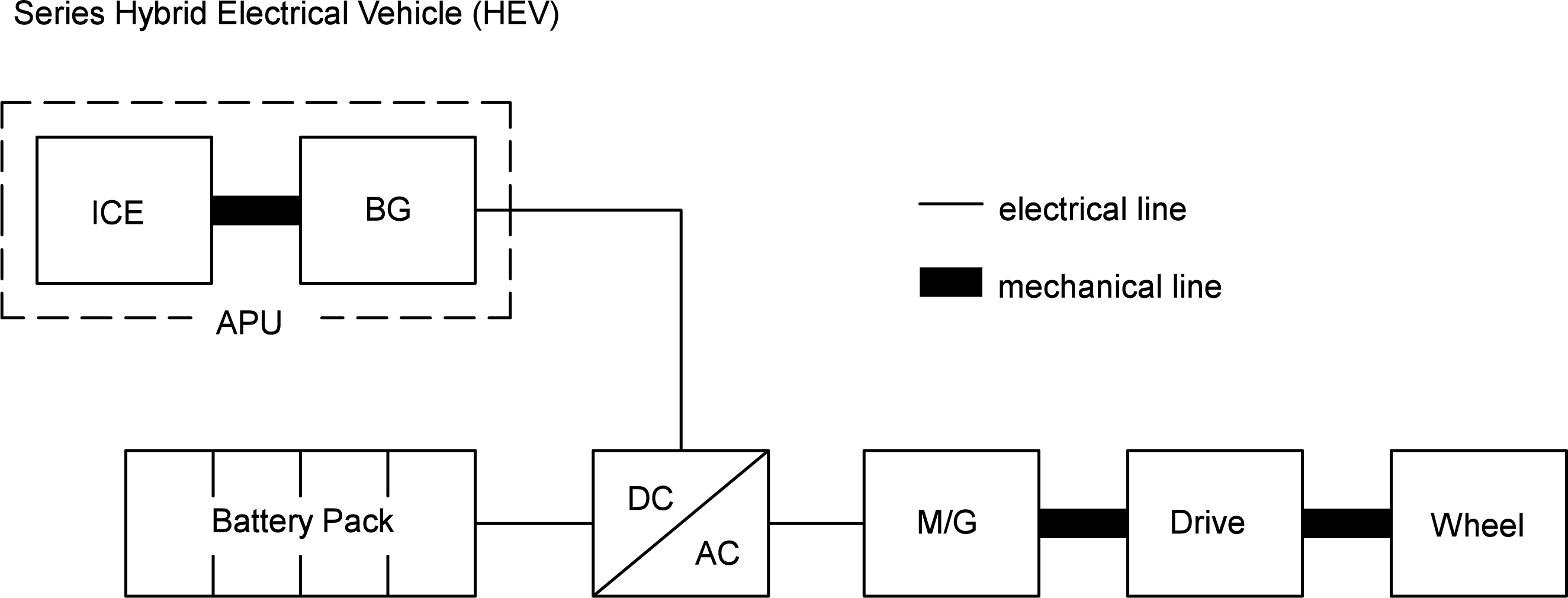
The hybrid electric powertrain is of the series type (Figure 1). In this kind of powertrain, there is no mechanical coupling between the electric motor-generator used for the application of the traction/braking torques to the wheels and the Internal Combustion Engine (ICE), which is used only to generate electricity. In HEVs, all of the ancillaries are driven by electric drives, because of the available electric storage. This assumption will be undertaken also for all the other powertrains under consideration in this paper (HM and TV). According to this assumption, one can suppose that the size of all of the ancillary devices is optimized for this purpose and that they usually work very close to their nominal working points with an advantage in terms of energy efficiency.

2.1.2. Gearbox

The gear drive between the electric motor and the wheel axle is characterized by a constant speed ratio i = ω_gb/ω_W = 6.2 and with the efficiency η_gb. Including the inertia torque of the shafts and the gears in T_W, the torque at gearbox T_gb = T_W/(iη_gb) in direct drive (T_W > 0) and T_gb = η_gbT_W/i in reverse drive are easily calculated.

2.1.3. Electric Motor-Generator

The electric motor-generator (M/G in Figure 1) must deliver all of the power that is necessary to fulfill the speed goal of the driving schedule; when necessary and if possible, it works also as a brake with a regenerative function. The motor-generator performs an electrical-mechanical energy conversion (or the reverse). By means of the efficiency maps of the motor-generator, the electrical power required or produced P_MG is given by:

$$P_{MG}=T_{gb}{\omega }_{gb}/{\eta }_{EM}$$

in direct drive and:

$$P_{MG}=T_{gb}{\omega }_{gb}{h\eta }_{EG}$$

in reverse drive, where η_EM = η_EM (ω_gb, T_gb) and η_EG = η_EG(ω_gb, T_gb) are the efficiency maps of the electric machine under motor or generator working conditions, respectively, and they are shown in Figure 2.

2.1.4. Power Electronics

The Alternating Current (AC) motor needs a conversion to Direct Current (DC) current for battery storage. Three electric paths are connected to the power electronics: the generator path, the motor path and the battery path. The energy balance (under stationary conditions) of the power electronics is given by the following equation:

$$P_{MG}^{\mathit{eff}}=P_{\mathit{APU}}+P_{\mathit{batt}}$$

where the P_APU is the electrical power from the auxiliary power unit and P_batt is the electrical power from the batteries. $P_{MG}^{\mathit{eff}}$ is the electrical power of the electric motor-generator, which takes also into account the power loss in power electronics (DC/AC in Figure 1). In fact, $P_{\mathit{MG}}^{\mathit{eff}}=P_{MG}/{\eta }_{PE}$ in direct drive and $P_{MG}^{\mathit{eff}}=P_{MG}{\eta }_{PE}$. The efficiency of the power electronics η_PE is given as a map of the actual working conditions.

2.1.5. Auxiliary Power Unit (APU)

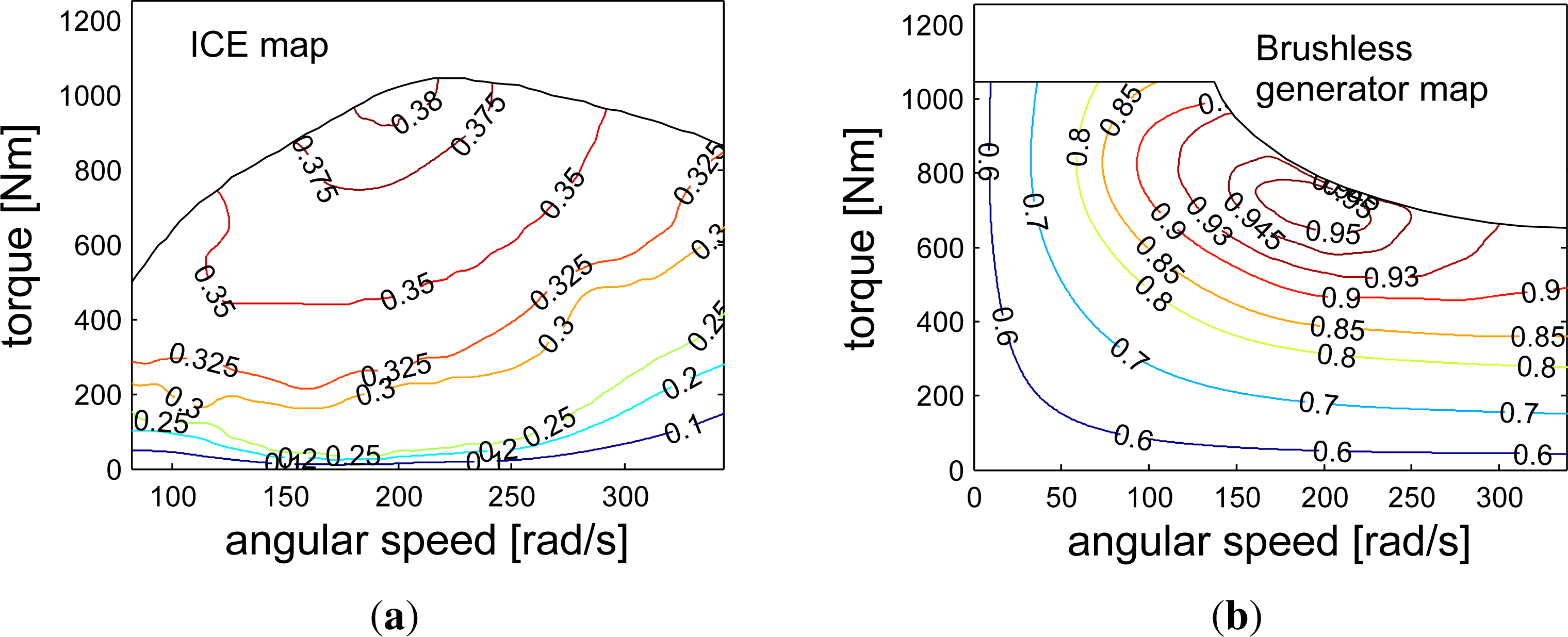
The APU of the hybrid electric powertrain is supposed to work at constant power at the optimal operating point of the thermal engine and the electric brushless generator. For this reason, the efficiency of the brushless generator (BG) and the specific fuel rate of the internal combustion engine (ICE) are both constants:

$$P_{\mathit{APU}}={\eta }_{BG}{P}_{ICE}$$

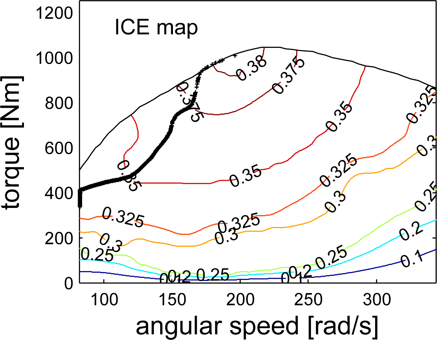
The efficiency map of both the ICE and the BG are shown in Figure 3.

2.1.6. Battery Pack

The electrical power P_batt flows in the battery path, and it is delivered or accumulated in the battery pack with the efficiency ${\eta }_{\mathit{batt}}^{\mathit{charge}}$ when charging and ${\eta }_{\mathit{batt}}^{\mathit{dicharge}}$ when discharging. It follows that the effective electrical power that is delivered from the batteries to the power electronics is:

$$P_{\mathit{batt}}^{\mathit{eff}}=\frac{P_{\mathit{batt}}}{{\eta }_{\mathit{batt}}^{\mathit{dicharge}}}$$

whereas the power that is actually accumulated in the batteries when charging is:

$$P_{\mathit{batt}}^{\mathit{eff}}={\eta }_{\mathit{batt}}{P}_{\mathit{batt}}$$

The state of charge (SOC) of the batteries is then defined as:

$$\mathit{SOC}={\int }_0^t{P}_{\mathit{batt}}^{\mathit{eff}}(t)\mathit{dt}+{\mathit{SOC}}_0$$

where SOC₀ is the initial value of the battery charge, and the power $P_{\mathit{batt}}^{\mathit{eff}}$ must be intended as positive in charge and negative in discharge.

2.2. Traditional Powertrain

A similar approach has been followed in the case of the traditional powertrain (Figure 4). Of course, in this case, the braking force that is necessary to decelerate the vehicle is given only by the friction brakes, since no regenerative braking is allowed by the ICE.

Moreover, the following simplifying assumptions are made: (1) all of the ancillaries are electrified, as in the case of HEV 2. The powetrain, conventionally made of a torque converter (TC) and an automatic 4–7 speed transmission with optimal management of the speed change will be supposed to achieve a continuous variation of the speed ratio, thus permitting the following of the Optimal Operating Line (OOL) of the ICE. The torque converter is considered in the simulation, with a proper lookup table. The assumed ideal transmission will give a slight underestimation of the fuel consumption with respect to real driving situations with a conventional powertrain. With this purpose in mind, this will not be a limitation for our results.

Furthermore, the engine is supposed to be turned on from the beginning till the end of the bus trip. This comes from the the experiments that have been carried out to measure the driving schedule. It has been observed that the engine is never switched-off, nor for long stops. Indeed, even if stop and re-start systems are commercially available for passenger cars, in the case of a bus, there are some technical issues due to the energy that must be provided to the ancillaries, so the application of stop and re-start systems is cumbersome in buses.

2.3. Mechanical Hybrid Powertrain

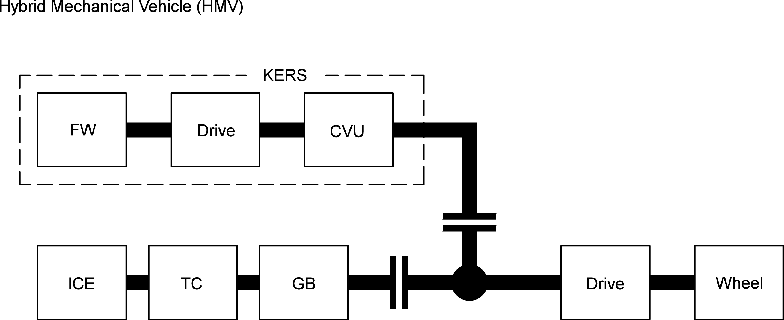
Mechanical hybrid bus (HMV) has also been simulated. A flywheel-based KERS has been proposed to be installed on the traditional powertrain line (equal to the one described in the previous section), as shown in Figure 1 of [20] and sketched in Figure 5. The mechanical KERS is made with a high-speed flywheel (12000–24000 RPM) driven by a Continuously Variable Transmission (with speed ratio τ_CVT, with ${\tau }_{\mathit{CVT}}^{\mathit{min}}<{\tau }_{\mathit{CVT}}<{\tau }_{\mathit{CVT}}^{\mathit{max}}$ with ${\tau }_{\mathit{CVT}}^{\mathit{min}}=0.4$ and ${\tau }_{\mathit{CVT}}^{\mathit{max}}=2.5$) and a fixed ratio drive (Drive in the KERS block in Figure 5) to speed down the high-speed flywheel shaft to the relatively low-speed propshaft of the vehicle.

A discussion about which type of Continuously Variable Unit (CVU) is to be preferred for the application to KERS is given in [20], where the possibility to use toroidal traction drives rather then shunted CVT architectures is investigated. It is there found that, disregarding the working power flow [12], the most convenient choice is the toroidal type variator, because of the relatively low efficiency of shunted CVT architectures, especially in reverse operation [19].

The speed ratio of the fixed ratio drive has been optimized following the approach described in [20]. An automatic friction clutch is also considered, which is used to manage the synchronization of the KERS shaft with the vehicle propshaft. The role of the CVU is to manage the power flow from the vehicle to the flywheel by changing the speed ratio. The CVU characteristics in terms of efficiency are similar to those described in [20], and the efficiency map is calculated as suggested in [26,27] for the full toroidal CVT.

By considering that the maximum energy that can be stored in the flywheel is $E_f^{\mathit{max}}=\frac{1}{2}{J}_f{\left({\omega }_f^{\mathit{max}}\right)}^2$, then the flywheel state of charge is defined as:

$$\mathit{SOC}=\frac{{\omega }_f^2}{{\left({\omega }_f^{\mathit{max}}\right)}^2}$$

The KERS works according to the following principles. If the vehicle must be speeded-up, the KERS clutch is engaged and the τ_CVT is changed in order to slow down the flywheel, speeding up the vehicle propshaft. This operating mode is allowed provided that: (1) the flywheel is charged ( ${\omega }_f>{\omega }_f^{\mathit{min}}$); and (2) a value of τ_CVT with ${\tau }_{\mathit{CVT}}^{\mathit{min}}<{\tau }_{\mathit{CVT}}<{\tau }_{CVT}^{\mathit{max}}$ exists, which permits synchronizing the KERS shaft with the vehicle propshaft with the given speed of the flywheel and the vehicle propshaft. On the other hand, the KERS is also used to slow down the vehicle (regenerative braking mode); in this case, the clutch is engaged and the τ_CVT is varied in order to speed up the flywheel and to slow down the vehicle. This operating mode is allowed provided that: (1) the flywheel charge is less the the maximum allowed charge ( ${\omega }_f<{\omega }_f^{\mathit{max}}$); and (2) a value of τ_CVT with ${\tau }_{\mathit{CVT}}^{\mathit{min}}<{\tau }_{\mathit{CVT}}<{\tau }_{\mathit{CVT}}^{\mathit{max}}$ exists, which permits synchronizing the KERS shaft with the vehicle propshaft with the given speed of the flywheel and the vehicle propshaft. Furthermore, also in the case of HMVs, the engine is supposed to be always turned on. For more details about the HM model, the reader is referred to [20], where all of the necessary equations may be found.

2.4. Ancillaries

The following ancillaries are considered and simulated to achieve a realistic calculation of the overall energy consumption of the bus:

(1)

Pressurized-air system (for opening doors, pneumatic suspensions, brakes, parking brake and other minor plants)

(2)

Hydro-Assisted steering system

(3)

Air heating-conditioning

(4)

ICE cooling system

(5)

Others (24 DC system)

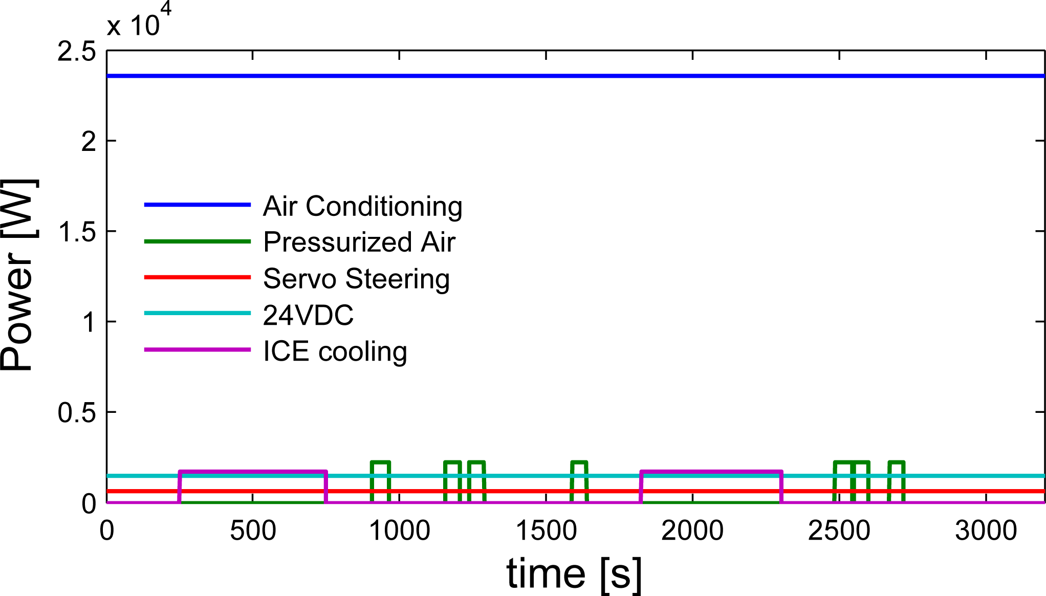
The energy consumption of all ancillaries is included in the simulations with the only exception being the air conditioning system, which will be simulated in both an “enabled” and “disabled” state. In fact, the energy consumption of the air conditioning system is very large (much larger than the others), and it will be shown that it very much affects the fuel consumption and, more importantly, the comparison of the performance of the powertrains under investigation. For this reason, following is a short description of how the energy consumption of the air cooling system has been calculated. An example of the results obtained for the HEV with air conditioning turned on is shown in Figure 6. It is shown that the air conditioning system, the servo steering system and the other 24 VDC auxiliaries are supposed to work with a constant power demand, whereas the ICE cooling system and the pressurized air system are intermittently turned on and off, depending on the actual need of the vehicle.

2.5. Air Conditioning System

The air conditioning system works under two different working conditions: heating and dry-cooling. In the former case, the hot water of the ICE cooling system is used to warm up the air in the bus cabin. In this working condition, the energy consumption is very, low because it is only due to a circulating pump for the hot water and air fans. The most energy-demanding systems among all the ancillaries is the air cooling system, so we investigated the fuel economy of traditional and hybrid buses in summer, when cooling is necessary for passenger comfort in the cabin. A typical summer working condition in the city of Taranto is considered, with the external temperature T_amb is equal to 35 °C and a solar radiation of I = 800 W/m². The cabin temperature T_bus is set equal to 25 °C. Under these conditions, the thermal balance of the bus cabin has been studied to calculate the energy that is necessary to keep the temperature equal to T_bus. It has been considered that one part of the bus external surface A_sun is exposed to sun light, whereas the other part A_shad is shadowed, with A_sun = 53 m² and A_shad = 63 m². Then, the thermal balance equations of the external surface of the cabin have been written for both sun-exposed and shadowed surfaces, respectively:

$$\begin{array}{c}{h}_{\mathit{rad}}^{\mathit{sun}}\left(T_{\mathit{surf}}^{\mathit{sun}}-T_{\mathit{sky}}\right)+h_{\mathit{conv}}\left(T_{\mathit{surf}}^{\mathit{sun}}-T_{\mathit{amb}}\right)+\frac{1}{R}\left(T_{\mathit{surf}}^{\mathit{sun}}-T_{\mathit{bus}}\right)=∊I\\ h_{\mathit{rad}}^{\mathit{shad}}\left(T_{\mathit{surf}}^{\mathit{shad}}-T_{\mathit{sky}}\right)+h_{\mathit{conv}}\left(T_{\mathit{surf}}^{\mathit{shad}}-T_{\mathit{amb}}\right)+\frac{1}{R}\left(T_{\mathit{surf}}^{\mathit{shad}}-T_{\mathit{bus}}\right)=0\end{array}$$

with: h_rad, h_conv, the radiation and convection coefficients, R the thermal resistance (conduction and internal convection) of the bus cabin walls, T_surf the temperature of the external surface of the bus walls, $T_{\mathit{sky}}=0.0552T_{\mathit{amb}}^{0.5}$ the sky temperature and ∊ = 0.9. The average thermal resistance of the cabin walls has been estimated taking into account the actual material composition of the bus walls (including glasses) and the internal convection coefficient. It results that 1/R = 7.09 W/(m² · °C). The convection coefficient h_conv has been calculated for an average speed of the bus of 5 m/s and an ambient temperature T_amb = 35 °C; it resulted that h_conv = 11.26 W/(m² · °C). The coefficient h_rad must be calculated with the following formula:

$$h_{\mathit{rad}}=∊\sigma \left(T_{\mathit{surf}}^2+T_{\mathit{sky}}^2\right)\left(T_{\mathit{surf}}+T_{\mathit{sky}}\right)$$

where σ = 5.67 × 10⁻⁸ W/(m² · K²) is the Stefan–Boltzmann constant ∊ = 1 and the surface temperature must be distinguished for sun-exposed and shadowed surfaces. Because the h_rad depends on the unknown temperature of the surface, the thermal balance equations are nonlinear equations to be solved in T_surf. It results that $h_{\mathit{rad}}^{\mathit{sun}}=6.4\hspace{0.17em}\text{W}/({\text{m}}^2\cdot °\text{C})$ and $T_{\mathit{surf}}^{\mathit{sun}}=59.3°\text{C}$, whereas $h_{\mathit{rad}}^{\mathit{shad}}=5.5\hspace{0.17em}\text{W}/({\text{m}}^2\cdot °\text{C})$ and $T_{\mathit{surf}}^{\mathit{shad}}=29.2°\text{C}$. Finally, the overall thermal balance equation of the bus cabin is:

$$Q_{\mathit{bus}}=Q_{\mathit{sun}}+Q_{\mathit{shad}}=\frac{A_{\mathit{sun}}}{R}\left(T_{\mathit{surf}}^{\mathit{sun}}-T_{\mathit{bus}}\right)+\frac{A_{\mathit{shad}}}{R}\left(T_{\mathit{surf}}^{\mathit{shad}}-T_{\mathit{bus}}\right)$$

from which it follows that Q_bus = 13.1 kW. In addition, the thermal power generated because of the greenhouse effect inside the bus cabin has been estimated Q_ghe = 5.8 kW. Finally, each passenger is supposed to radiate about q_pass = 50 W. By considering n_pass = 30 passengers on average, it results that Q_pass = n_passq_pass = 1.5 kW. The power needed to cool the cabin in summer is: Q = Q_pass + Q_bus + Q_ghe = 20.4 kW. The energy consumption of the cooling system has been estimated by considering that the efficiency of the compressor to be about equal to η_compressor = 0.865. It must be noticed that in the present investigation, all of the ancillaries are supposed to be electrified also in the case of HM and TV powertrains, whereas at the present state of the art, HVAC systems with high efficiency are used only in HEV. The aforementioned assumption makes more sense for the HM buses, which are not currently on the market, so that it is reasonable that future designs can also include this characteristic. In the case of TV, this assumption leads to an underestimation of the actual fuel consumption of the vehicles that are currently on the market. However, such an assumption is also in agreement with other ones made in this paper, for instance the ideal CVT transmission that permits the ICE to always work close to the optimal operating line. In this sense, the TV simulated in this paper can be considered as one possible future development of the TV currently on the market.

3. Real Driving Schedule: Urban Bus in the City of Taranto

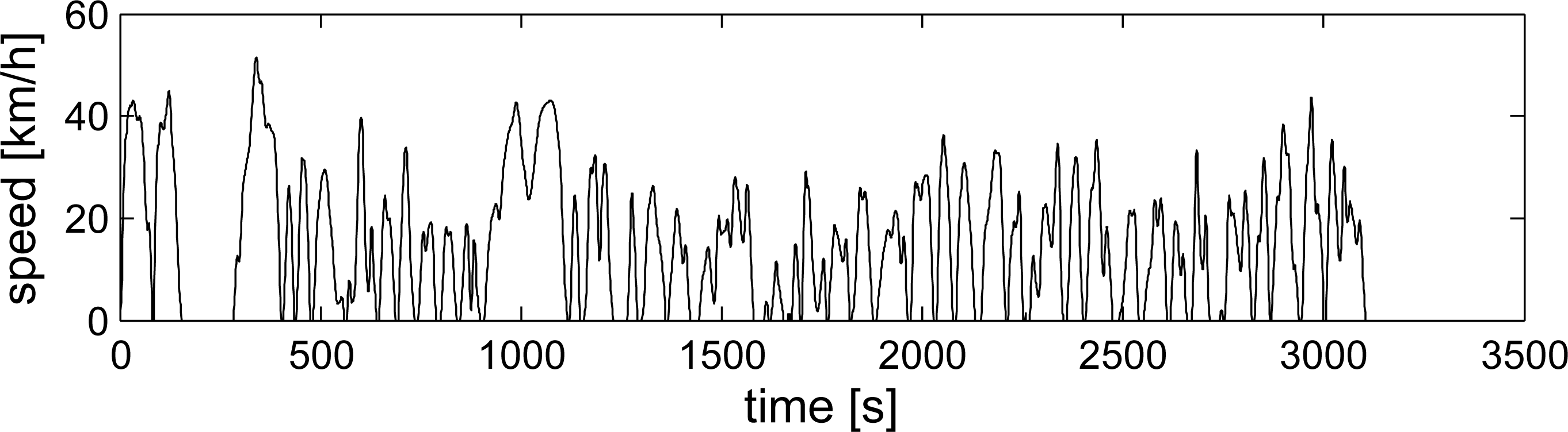
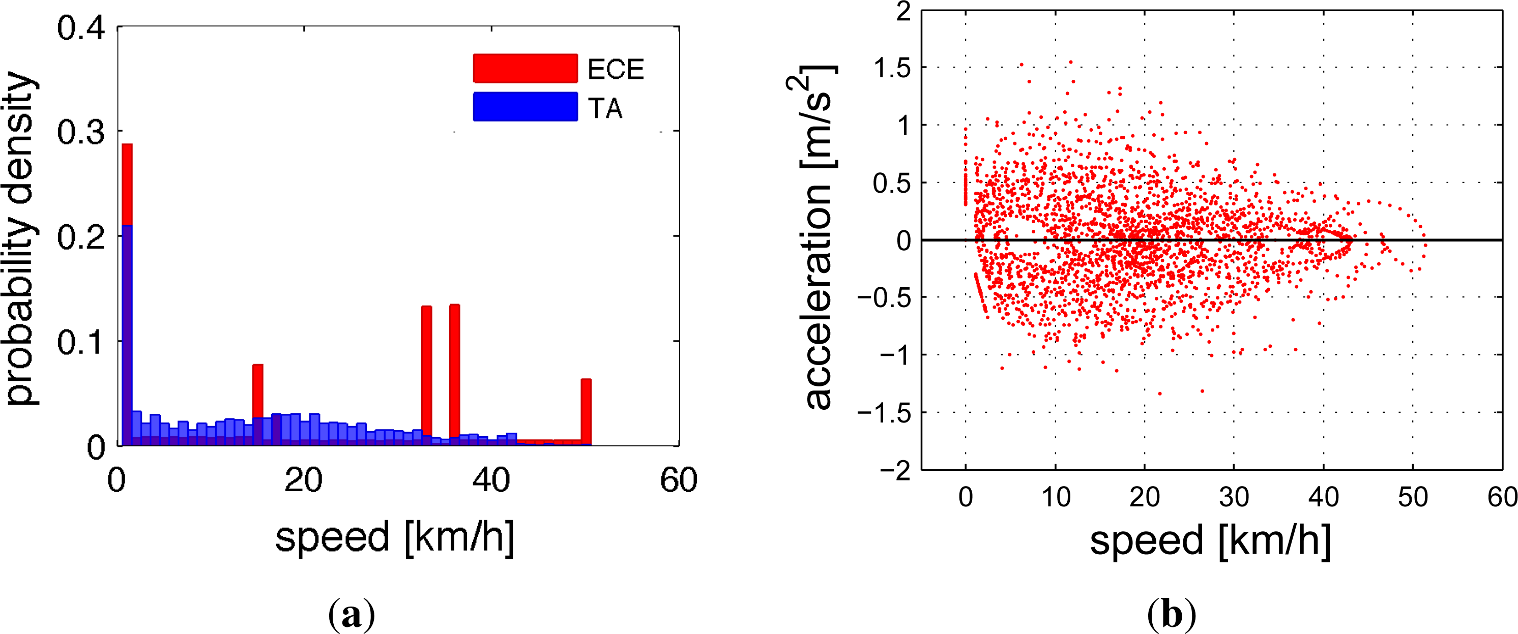
Inverse dynamic simulations for the calculation of the bus vehicle fuel economy need a realistic driving schedule. In this paper, the driving schedule was obtained measuring the typical velocity profile of an urban bus in the city of Taranto, Italy (see Figure 7). The bus route that was chosen travels across the town, starting from a peripheral urban area; thus, it represents all possible traffic conditions well. The velocity was measured and recorded through a Global Positioning System (GPS) and a notebook at one sample per second. The velocity profile obtained through this technique has been post-processed to eliminate some measurement errors due to the GPS signal (GPS signal lost, single value errors with positive or negative non-physical peaks of velocity, etc.). Several measurements were performed on the same bus route, on different days of the week and in three different periods of the day. A statistical analysis of the measurements reveal that for one given period of the day, the probability distribution of the velocity is always similar to Figure 8a. Figure 8a shows the probability density distribution of the bus speed of the velocity profile shown in Figure 7. Figure 8b shows the acceleration vs. speed of the analyzed drive schedule. A peak positive acceleration of 1.6 m/s² and a negative peak of 1.4 m/s² have been recorded, with a peak bus speed of 51 km/h. In Figure 8a, it is shown that the vehicle speed distribution has a peak for v = 0, which corresponds to a stationary condition (with the engine turned on in the case of the real bus). The probability density distribution of the bus speed for the standard European Driving Cycle ECE cycle is also shown in Figure 8a for comparison. The two distributions are very different from each other, because in real driving situations, the bus never travels at a constant speed for a long time, so the real distribution is quite flat over a large part of the speed range. This is the reason why, for the purposes of this paper, it was preferred to measure the typical driving schedule on the road rather than using standard cycles.

4. Simulation Results

The driving schedule of the city of Taranto (see Figure 7) has been simulated with the three different aforementioned powertrains: traditional vehicle (TV); hybrid mechanical vehicle (HMV) and hybrid electric vehicle (HEV). The simulations have been performed through a numerical code developed for this purpose. The bus has the general characteristics listed in

Table 1. Vehicle characteristics and other constants.

Quantity	Symbol	Value
vehicle overall mass (with passengers)	m*	15, 300 kg
tire radius	RW	0.4783 m
air density	ρ	1.23 kg/m
acceleration of gravity	g	9.81 m/s2
frontal vehicle surface	Af	8.25 m2
drag coefficient	cd	0.7
rolling friction coefficient	cr	0.008
road slope	β	0

. All of the ancillaries have been simulated, and in particular, two conditions have been considered for the air cooling system, which are: (1) an enabled system with ambient temperature equal to 35 °C and an internal bus temperature equal to 25 °C; (2) disabled. It has been estimated that the additional power supply needed in the enabled state is about of 20.4 kW, which has been considered constant during the bus operation.

The engine usage map and the fuel flow rate for the bus powered by the traditional powertrain are shown in the Figures 9 and 10. The simulations have been performed assuming that the engine is kept turned on during vehicle stops (a condition that has been observed on the road), so that the flow rate is supposed to be never zero. Furthermore, it has been supposed that the transmission always permits working very close to the optimal operating line of the engine, and so, the working points on the engine usage map are always very close to that line (Figure 9). Turning on the air cooling system has the main effect of pushing the fuel flow rate curve upwards over the entire time range. The engine usage map does not change if the air cooling system is enabled or disabled, because the transmission always allows following the optimal operating line.

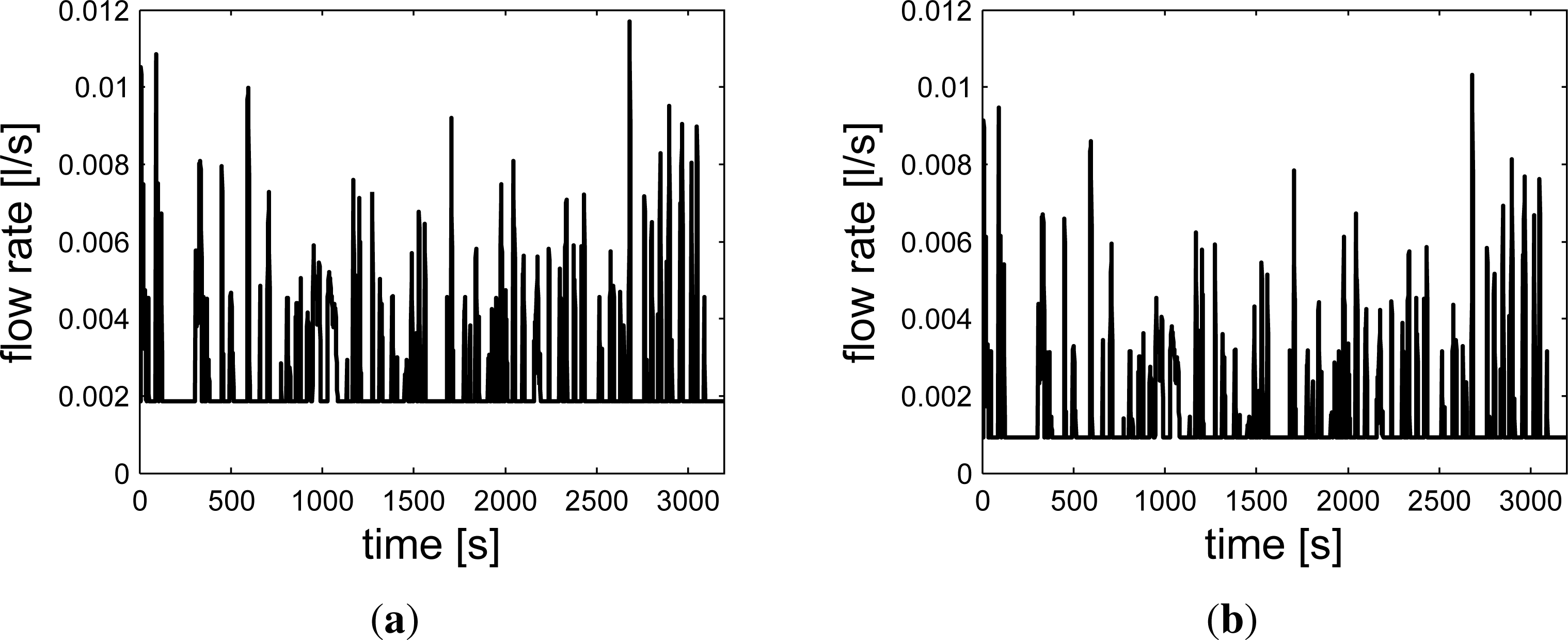
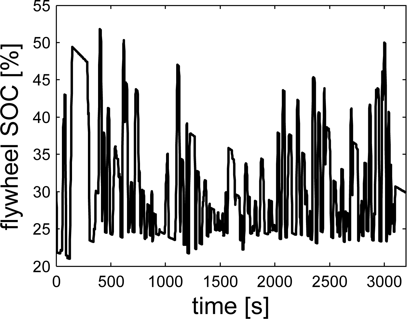
Figure 11 shows the fuel flow rate with both (1) an enabled and (2) a disabled air cooling system. The flow rate is qualitatively similar to the traditional powertrain bus, sometimes with visibly lower values, because of the torque assist provided by the flywheel KERS. The State of Charge (SOC) of the KERS, defined as the ratio between the effective kinetic energy stored in the flywheel divided by the maximum storable kinetic energy $\text{SOC}={\omega }_f^2/{\omega }_{f\mathit{max}}^2$, is shown in Figure 12.

The simulated KERS is designed to recover the energy of the bus at about 60 kph, so it is shown how the SOC never exceeds 50%, because the bus speed in the selected route never exceeds 50 kph. We observed that the SOC is not affected by the enable state of the air conditioning system, because the power requirement of the KERS is mainly affected by the acceleration or deceleration of the vehicle. The engine usage map of the KERS powertrain is not shown, because it is very similar to the traditional powertrain, since it is supposed that the continuously variable transmission allows following the optimal operating line of the engine map.

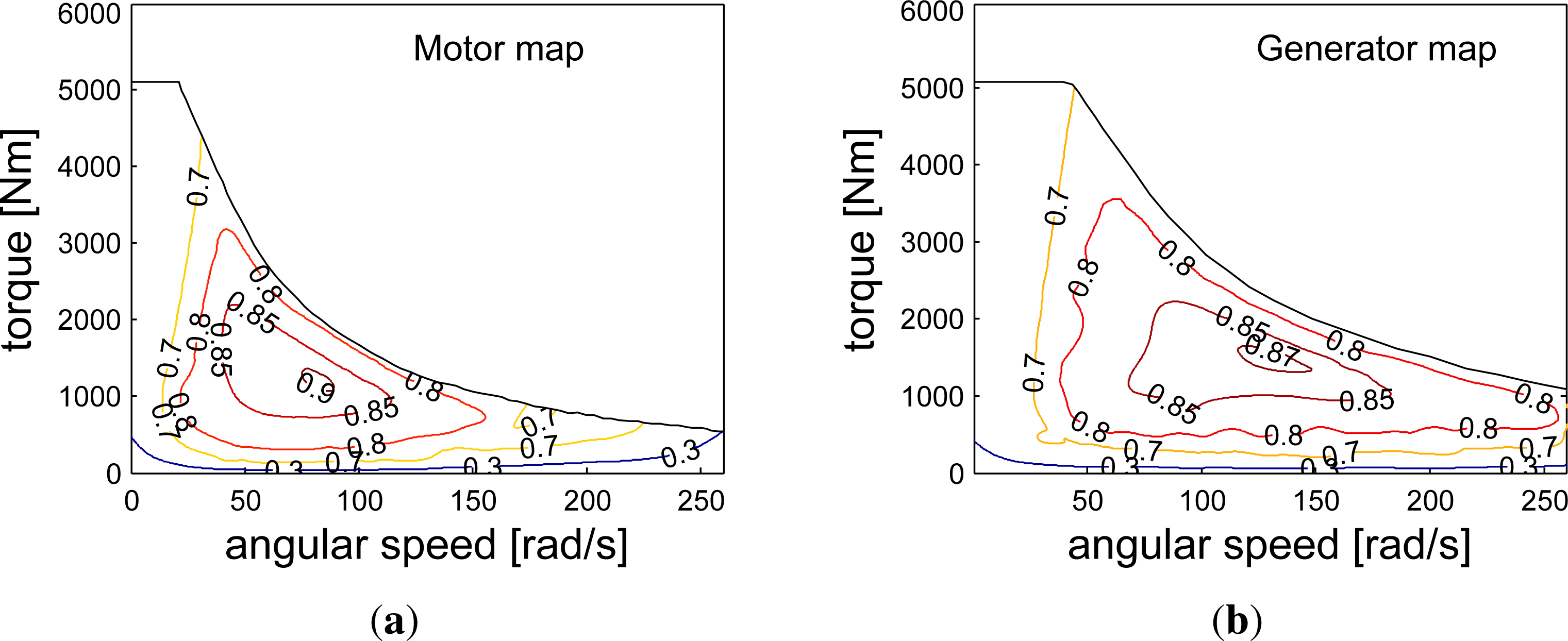
The HEV has been simulated under the same working conditions of the other powertrains. Figure 13 shows the usage maps of the induction motor/generator, the ICE and the brushless generator. In particular, the APU works at a fixed point, which corresponds to the maximum efficiency condition, whereas the working points of the induction motor/generator depend on the vehicle speed and torque needed. It can be shown that in urban drive, the average efficiency of the induction motor is low (<0.7), because it very often happens that the torque required is quite small. In the HEV, the APU is driven in order to keep the SOC of the batteries always between a minimum and a maximum corresponding to 20% to 80%. When the battery pack is charged, the APU is turned-off until the SOC falls beneath the minimum allowed value; then the APU is turned on again.

Figure 14 shows the fuel flow rate of ICE in the case of a series HEV with (1) the cooling system turned on and (2) off. The ICE is regulated on-off, and when turned-on, it delivers constant power and torque; so, also the flow rate is constant. Comparing the time history of the flow rate in the two cases with and without air-conditioning, it immediately follows that the overall fuel volume to complete one trip is more than double if the air conditioning system is turned on, since the APU must be switched on two times in a trip for a longer time. It is clearly seen from the battery SOC (Figure 15) that one charge is almost enough to make one trip if the AC is turned off, whereas it is necessary to recharge the batteries at half-trip if the AC system is turned on.

In the end, the fuel consumption given by the three different powertrains is shown in Figure 16. In the case with the AC turned off, it is obtained that the HEV gives the best fuel economy performance, with respect to either the HMV (−25%) and the TV (−35%). This result was expected for several reasons. Among all, the main reason is that the urban drive is characterized by small power requirements, because of the small speed values, which corresponds to the relatively low efficiency of the ICE. In this case, the advantage of the HEV is that it makes it work always at its best efficiency; moreover, in the HEV, the ICE is turned off when it is not necessary to recharge the batteries, and regenerative braking is also performed. The calculated advantage achieved by HEV over TV (−35% fuel consumption) is also in agreement with some results found in the literature [3]. The HMV gives intermediate results between the HEV and the TV, mainly because of energy recovery.

On the other hand, when the AC is turned on, then the situation is different. In fact, the fuel economy performance of the HEV is dramatically lost, since the fuel consumption is increased by 142% in the HEV powertrain, whereas it increases only by 73% for the HMV and 68% for the TV. In absolute terms, the HEV is not yet the most energy-efficient system, because it is slightly overcome by the HMV. The reason for that is related to the efficiency of the ICE in both the HMV and TV. Because of the larger average power required, the ICE works with a larger average efficiency than with the AC system turned off. On the other hand, the overall efficiency of the HEV is, in general, decreased, because, despite nothing changing for the induction motor/generator, much more power must be generated by the APU, which also means much more energy loss in all of the electric branch of the powertrain as a consequence of the non-unitary efficiency of all of the devices. Such an increase of power loss is not even partly compensated by an increase of the efficiency of the ICE, since it still works with fixed and optimal working conditions.

5. Conclusions

In the last few years, hybrid vehicles have been considered as one possible solution in the short–medium range for improving the fuel economy and reducing the polluting emissions of road vehicles. Furthermore, hybrid buses have been developed and put into mainstream production, with the hope of replacing the elder existing diesel engine-powered vehicles, which causes the emission of great quantities of particulate. In this paper, the fuel economy of series hybrid-electric and hybrid-mechanical buses has been simulated in real driving situations. Driving in the city of Taranto, a city in Southern Italy, has been investigated in two conditions: cold weather and hot weather. The analysis has been carried out by an inverse dynamic approach. The bus speed is given as a velocity pattern, which comes from on-road measurements performed on one of the present city bus routes. The city of Taranto drive schedule has been simulated considering two different seasons: one with a cold weather, when the air conditioning system is switched off, and one with hot weather, when the air conditioning system must be switched on for passengers’ comfort. The fuel consumption of hybrid electric and hybrid mechanical buses are compared to each other and with a traditional bus powered by a diesel engine. All vehicles are powered by the same diesel ICE. It is shown that the series hybrid-electric vehicle outperforms both the traditional and the mechanical hybrid vehicles in the simulations with the air conditioning system turned off, showing that the fuel consumption is about 35% less than the traditional diesel bus and 25% less then the mechanical hybrid bus. On the other hand, it is also shown that the performance of the hybrid-electric bus gets dramatically worse with hot weather (+142% fuel consumption), when, as a consequence of the large power demand of the air-cooling system, its average efficiency is much less than in the former case. In this situation, it is found that the fuel consumptions of the three buses under investigation are comparable. The best fuel economy was achieved with the mechanical hybrid bus, which takes advantage of the increased power required for the ICE, which works with larger average efficiency in this case.

References

- Kellaway, M.J. Hybrid buses—What their batteries really need to do. J. Power Sources 2007, 168, 95–98. [Google Scholar]
- Van den Bossche, P. Power sources for hybrid buses: Comparative evaluation of the state of the art. J. Power Sources 1999, 80, 213–216. [Google Scholar]
- Sangtarash, F.; Esfahanian, V.; Nehzati, H.; Haddadi, S.; Bavanpour, M.A.; Haghpanah, B. Effect of Different Regenerative Braking Strategies on Braking Performance and Fuel Economy in a Hybrid Electric Bus Employing CRUISE Vehicle Simulation. SAE Int. J. Fuels Lubr 2009, 1, 828–837. [Google Scholar]
- Wu, Y.Y.; Chen, B.C.; Huang, K.D. The Effects of Control Strategy and Driving Pattern on the Fuel Economy and Exhaust Emissions of a Hybrid Electric Bus; SAE Technical Paper 2008-01-0306; SAE International: Warrendale, PA, USA, 2008. [Google Scholar]
- Qin, K.; Li, M.; Gao, J.; Gao, J.; Ai, Y. On-Road Test and Evaluation of Emissions and Fuel Economy of the Hybrid Electric Bus; SAE Technical Paper 2009-01-1866; SAE International: Warrendale, PA, USA, 2009. [Google Scholar]
- Hu, H.; Zou, Z.; Yang, H. On-board Measurements of City Buses with Hybrid Electric Powertrain, Conventional Diesel and LPG Engines; SAE Technical Paper 2009-01-2719; SAE International: Warrendale, PA, USA, 2009. [Google Scholar]
- Xiong, W.; Zhang, Y.; Yin, C. Optimal energy managemnt for a series-parallel hybrid electric bus. Energy Convers. Manag 2009, 50, 1730–1738. [Google Scholar]
- Xiaohua, Z.; Qingnian, W.; Weihua, W.; Liang, C. Analysis and Simulation of Conventional Transit Bus Energy Loss and Hybrid Transit Bus Energy Saving; SAE Technical Paper 2005-01-1173; SAE International: Warrendale, PA, USA, 2005. [Google Scholar]
- Millo, F.; Fuso, R.; Rolando, L.; Zhao, J.; Benedetto, A.; Cappadona, F.; Seglie, P. HYBUS: A New Hybrid Bus for Urban Public Transportation; SAE Technical Paper 2013-24-0081; SAE International: Warrendale, PA, USA, 2013. [Google Scholar]
- Rohde, S.; Schilke, N. The Fuel Economy Potential of Heat Engine/Flywheel Hybrid Vehicles; SAE Technical Paper 810264; SAE International: Warrendale, PA, USA, 1981. [Google Scholar]
- Brockbank, C.; Greenwood, C. Fuel Economy Benefits of a Flywheel & CVT Based Mechanical Hybrid for City Bus and Commercial Vehicle Applications. SAE Int. J. Commer. Veh 2009, 2, 115–122. [Google Scholar]
- Mangialardi, L.; Mantriota, G. Power flows and efficiency in infinitely variable transmissions. Mech. Mach. Theory 1999, 34, 973–994. [Google Scholar]
- Mantriota, G. Theoretical and experimental study of a power split continuously variable transmission system Part 1. Proc. Inst. Mech. Eng. Part D J. Autom. Eng 2001, 215, 837–850. [Google Scholar]
- Mantriota, G. Theoretical and experimental study of a power split continuously variable transmission system Part 2. Proc. Inst. Mech. Eng. Part D J. Autom. Eng 2001, 215, 851–864. [Google Scholar]
- Mantriota, G. Performances of a series infinitely variable transmission with type I power flow. Mech. Mach. Theory 2002, 37, 579–597. [Google Scholar]
- Mantriota, G. Performances of a parallel infinitely variable transmissions with a type II power flow. Mech. Mach. Theory 2002, 37, 555–578. [Google Scholar]
- De Pinto, S.; Mantriota, G. A simple model for compound split transmissions. Proc. Inst. Mech. Eng. Part D J. Autom. Eng 2014, 228, 549–564. [Google Scholar]
- Bottiglione, F.; de Pinto, S.; Mantriota, G. Infinitely Variable Transmissions in neutral gear: Torque ratio and power re-circulation. Mech. Mach. Theor 2014, 74, 285–298. [Google Scholar]
- Bottiglione, F.; Mantriota, G. Reversibility of Power-Split Transmissions. ASME J. Mech. Des 2011, 133, 084503:1–084503:5. [Google Scholar]
- Bottiglione, F.; Mantriota, G. Effect of the ratio spread of CVU in automotive kinetic energy recovery systems. J. Mech. Des 2013, 135, 061001:1–061001:9. [Google Scholar]
- Bottiglione, F.; Carbone, G.; de Novellis, L.; Mangialardi, L.; Mantriota, G. Mechanical hybrid KERS based on toroidal traction drives: An example of smart tribological design to improve terrestrial vehicle performance. Adv. Tribol 2013, 2013, 918387:1–918387:9. [Google Scholar]
- Bottiglione, F.; Mantriota, G. MG-IVT: An infinitely variable transmission with optimal power flows. J. Mech. Des 2008, 130, 112603:1–112603:10. [Google Scholar]
- Wu, B.; Lin, C.C.; Filipi, Z.; Peng, H.; Assanis, D. Optimal power management for a hydraulic hybrid delivery truck. Veh. Syst. Dyn 2004, 42, 23–40. [Google Scholar]
- Yan, Y.; Liu, G.; Chen, J. Integrated modeling and optimization of a parallel hydraulic hybrid bus. Int. J. Autom. Technol 2010, 11, 97–104. [Google Scholar]
- Guzzella, L.; Sciarretta, A. Vehicle Propulsion Systems; Springer-Verlag: Berlin, Germany, 2010. [Google Scholar]
- Carbone, G.; Mangialardi, L.; Mantriota, G. A comparison of the performances of full and half toroidal traction drives. Mech. Mach. Theory 2004, 39, 921–942. [Google Scholar]
- De Novellis, L.; Carbone, G.; Mangialardi, L. Traction and Efficiency Performance of the Double Roller Full Toroidal Variator: A Comparison with Half- and Full- Toroidal Drives. ASME J. Mech. Des 2012, 134, 071005:1–071005:14. [Google Scholar]