On the Design and Response of Domestic Ground-Source Heat Pumps in the UK

Faculty of Engineering & Environment, Northumbria University, Newcastle NE1 8ST, UK
Energies 2014, 7(7), 4532-4553; https://doi.org/10.3390/en7074532
Submission received: 30 April 2014
/
Revised: 7 July 2014
/
Accepted: 9 July 2014
/
Published: 15 July 2014
(This article belongs to the Special Issue Geothermal Energy: Delivering on the Global Potential)
Abstract
:The design and response of ground source heat pumps coupled to vertical closed loop arrays in UK domestic applications are investigated in this article. Two typical UK house types are selected as the vehicle for the study and a detailed dynamic thermal modelling method is used to arrive at time-series heating demands for the two houses. A new empirical heat pump model is derived using experimental data taking into account the deteriorating performance of the heat pump during periods of light load. The heat pump model is incorporated into an existing numerical ground model and completed with a classical effectiveness type heat exchange model of the closed loop array. The model is used to analyse array sizing and performance over an extended time period, as well as sensitivity of the design to soil conductivity and borehole heat exchanger resistance and sensitivity to over-sizing and part-load behavior of the heat pump. Results show that the UK’s standard for ground source design (the Microgeneration Certification Scheme) may lead to under-estimated array sizes and that heating system over-sizing and deleterious part-load heat pump performance can add up to 20% to the electrical consumption of these systems.
1. Introduction
During the first phase of recent UK field trials on 81 domestic air- and ground-source heat pumps the median seasonal performance factor (SPF) of the sample of 54 ground source heat pumps was found to be 2.2 [1]. (In this context, the seasonal performance factor is taken to mean the heat delivered to the space heating and domestic hot water service over a complete annual operating cycle divided by the corresponding electricity required by the heat pump and its associated source and sink circulating pumps.) The performance was well below expectations and was attributed to a multitude of factors including system sizing, type of source, building efficiency, user behavior and installation practices. Following the first phase of these trials, several site interventions were planned and improvements to the Microgeneration Certification Scheme (MCS) [2] were made to inform future users of heat pumps on procedures for design and installation. The interventions ranged from minor measures (e.g., adjustments to controls) to major interventions (in some cases, involving a re-installation of the heat pump or radiators where they were considered inappropriately sized). Following the interventions, a sample of 32 improved installations were monitored for one further year of which 21 were ground source heat pumps. The median SPF for this sample was found to be 3.1 [3]. Whilst the improvement in seasonal coefficient of performance to 3.1 is welcome, it is still short of the potential for these systems. Most of the domestic heat pumps available at present use a remarkably similar kit of parts. These include brazed plate heat exchangers for the evaporator and condenser (which tend to give better heat exchange “pinch” than the first-generation shell and tube heat exchangers), scroll fixed-speed compressors and mechanical (“thermostatic”) expansion devices. A buffer water store on the heating side is usually included either as part of the heat pump package or plumbed-in separately and the control of the heat pump is usually by means of a heating thermostat mounted in the heating flow from the heat pump (though often in the heating return especially when a buffer tank is not used). Therefore, it is to be expected that variations of the kind identified in [1,2] are most likely to be due to design, installation and operational issues rather than issues concerned with the heat pump itself.
The UK experiences a quite different climate than that experienced in continental regions in that its weather is governed by maritime conditions with mild winters and frequent episodes of abrupt variations in weather from day to day. Partly because of this, lower standards of thermal insulation tend to be used in UK building construction than is the case in colder climatic regions. It is also generally accepted that the UK lags behind continental Europe and America in its exploitation of ground source heat (though the recent introduction of tariff incentives is likely to see that situation change quite abruptly in the coming years). The UK’s geological formations (many of which are at least moderately water-bearing) are also quite different to many of the well-drained sites in America where closed loop ground source heat pumps have been widely used and reported. To account for this, reference will be made in this work to a new and large data set of ground formation conductivities from a large number of sites across the UK. Thus, UK conditions for the use of ground source heating offer a number of unique features which make detailed research and evaluation particularly timely.
In this work, the impact of heat pump capacity and ground array design for domestic ground source heat pumps operating in UK conditions are explored in detail with a view to establishing design criteria that might lead to improvements in operating performance. This will be achieved through the following objectives:
- Detailed dynamic modelling of two typical UK house types of differing sizes and energy demands.
- Development of a new empirical heat pump model which accounts for the degradation in part-load operating performance evident in these systems.
- Design of vertical ground loop arrays using the simulated house energy demands and the new heat pump model.
- Investigations into the sensitivity of the array designs to variations in soil and borehole heat exchanger properties and an analysis of the robustness of the designs over an extended operating time horizon (5 years).
- Investigations into the sensitivity of the seasonal heat pump electrical energy use and house comfort conditions to the under-sizing and over-sizing of the heating system.
Previous Work
Bagdanavicius and Jenkins [4] modelled electrical energy demands for a community of 96 two, three and four-bedroom houses with the assumption that all of the houses used a ground source heat pump sized according to the MCS heat pump standard [2]. They found domestic hot water energy use to have a major bearing on results but their results were restricted to just one winter week. In an experimental study, Blanco et al. report on the performance of a variable speed compressor-driven heat pump at domestic scale [5]. Variable speed heat pumps are yet to be widely adopted at domestic scale and are likely to bring part-load performance improvements as well as dispensing with the need for sink-side buffer heat storage. They found that, on average, the electrical consumption when operating with heating temperatures of 35 °C was 29% lower than when operating at 45 °C. Wood et al. carried out an experimental investigation into a vertical ground array consisting of single “U-tubes” cast into 10 m-deep piles [6]. They used 21 such piles making an overall array size of 210 m and demonstrated a typical heating delivery rate of 6 kW with a seasonal performance factor of 3.62. So called “energy piles” can provide strong economic advantages compared with conventional vertical ground source arrays though this method of foundation construction is seldom used in house construction. Boait et al. investigated the performance of a group of bungalows equipped with ground source heat pumps [7]. They obtained results that were consistent with the first phase of the Energy Saving Trust’s trials mentioned earlier [1] and, again, revealed performances that were below observations from other field trials carried out elsewhere in continental Europe. This conclusion is also comprehensively arrived at by a detailed analysis of a number of European field trials on both air- and ground-source heat pumps carried out by Gleeson and Lowe [8]. One of a number of reasons for the performance shortfall mentioned in the Boait et al. study was the limited availability of very low capacity heat pumps for small well-insulated UK dwellings (such as bungalows) meaning that the larger capacity heat pumps that are used tend to operate for long periods at light load. However the overarching finding from all of these sources is that the reasons for the disappointing UK performances are complex and multi-faceted and further work is needed.
In conclusion, evidence is beginning to emerge which suggests that domestic ground source heat pumps in the UK are performing below expectations and below comparable installations in other parts of Europe. It appears that there are many reasons for this but a key consideration would appear to be the capacity of the heat pumps used in the UK in relation to the pattern of domestic energy demand. Matters are complicated by the requirement to generate domestic hot water through the summer months when space heating is usually not required. This is often at temperatures that are higher than would be required for space heating due to the need to ensure safe hygiene standards in hot water storage and plumbing systems (though this can be conveniently addressed with minimal loss in performance through the use of a two-zone de-superheater/condenser [5,9]).
2. Energy Demand Modelling in a Sample of UK Houses
2.1. House Type Selection and Seasonal Modelling
Nearly 55% of the 2.8 million UK houses surveyed in 2010 and reported in the National Energy Efficiency Data Framework (NEED) [10] had gross floor areas of between 51 m2 and 100 m2 and the next largest group (29%) had gross floor areas of between 101 m2 and 150 m2. The mean gas consumptions of these two groups in 2010 were 13,200 kWh and 18,000 kWh, respectively, which, with a well-maintained gas boiler efficiency of 0.85, can be considered to translate to thermal energy demands of 11,220 kWh and 15,300 kWh, respectively. Two house types with gross floor areas of 75 m2 and 125 m2 were therefore chosen to fall within this range. It was assumed that the first of these would be a two-story mid-terrace house and the second would be a two-story detached house. Simplified seasonal energy demand modelling was carried out using BREDEM 2012 [11].
Briefly, BREDEM 2012 [11] “Building Research Establishment Domestic Energy Model” is a calculation procedure to estimate all forms of energy consumption in houses. It is a monthly calculation method based on monthly-averaged weather data. The house to be modelled is split into two zones—a main living zone (usually the living room or main reception room) and the rest of the house forms a second balance zone. A simple time-constant-based model is used to estimate heating energy use whereas regression-fitted models based on observations of a large number of UK house types are used to calculate hot water and electrical equipment energy demands. Though the electrical demands are of no direct interest in the present work, they are indirectly used to provide information on internal heat gains which are used to adjust space heating demands. Mainly because of the regression models for energy uses that would otherwise be very difficult to calculate theoretically, BREDEM 2012 [12] tends to give highly representative and accurate results over longer-term averaging periods in strictly UK conditions but is not suitable for energy studies over short time periods. The methods described in BREDEM 2012 [11] form the primary methods used in all UK domestic energy planning and design evaluation work.
Adjustments were made to house layout, glazing and construction details such that results from the BREDEM modelling provided values that were similar to the two mean gas consumptions from the NEED data [10] with the intention of arriving at two “very typical” UK house types as judged by energy demand performance. The details arrived at in this way are consistent with houses that were either constructed or fully refurbished to standards prevailing at about the beginning of this century.
Thermal properties and other details of the two house types can be found in Appendix A (Table A1 and Table A2).
Results of the BREDEM modelling using a London site selection for both houses are summarized in Table 1. The totals given in Table 1 can be seen to be of the order of the NEED results mentioned above and can thus be considered to be representative of commonly occurring UK house types of this scale.

| House Type | Space Heating (kWh) | Domestic Hot Water (kWh) | Total (kWh) |
|---|---|---|---|
| Mid-terrace | 7,764 | 2,983 | 10,747 |
| Detached | 13,556 | 3,377 | 16,933 |
2.2. Dynamic Thermal Modelling
The BREDEM results give a good representation of annual energy demand in UK housing which is why the methods used are linked to the Standard Assessment Procedure (SAP) for the purposes of energy efficiency policy development, design and planning applications in the UK. The method is, however, limited in that for the detailed analysis of renewable, low carbon and other complex microgenerators, more granular time-series results of energy demand data are required (e.g., half-hourly or hourly data) whereas BREDEM is only able to provide results at monthly (minimum) intervals. For loads that can be considered to follow a daily average pattern such as domestic hot water this is of no consequence but for the dominant energy demand due to space heating which varies due to both climate and user activity this is a serious limitation. Indeed the need to achieve a better understanding of the response of the heat pump and heating system with the dynamics of the building were emphasised by Boait et al. in their field trial study [7]. The two house types were thus remodeled using a dynamic thermal modelling procedure and the results compared for accuracy with the BREDEM reference results.
Re-modelling of the space heating energy use for both houses was carried out using a superset of bespoke building energy modeling components developed for Simulink in the Matlab environment—the Simulink HVAC (heating, ventilating and air conditioning) Blockset. Details of the blockset library can be found in Appendix B (Figure B1 and Figure B2) and details of the mathematical derivations of the most relevant blocks used in the present work can be found in the literature [12,13]. All dimensional and other details as were used in the BREDEM modelling were also used in the dynamic thermal modelling (Appendix A). A current test reference year weather file for London was used from the Chartered Institution of Building Services Engineers (CIBSE) Future Weather Years set [14]. (Note that monthly-average values from this weather file were also used in the earlier BREDEM modelling.)
For domestic hot water energy, the original BREDEM monthly predictions were broken down into daily average values. The operating daily schedules were then applied which consisted of one 2 h heating period each weekday morning following by one 7 h heating period during each weekday evening. On weekend days, one single 16 h heating period was applied. The domestic hot water loads were allocated to the morning and evening periods in the ratio of 1:2, respectively (this pattern was assumed to apply on both weekdays and weekend days).
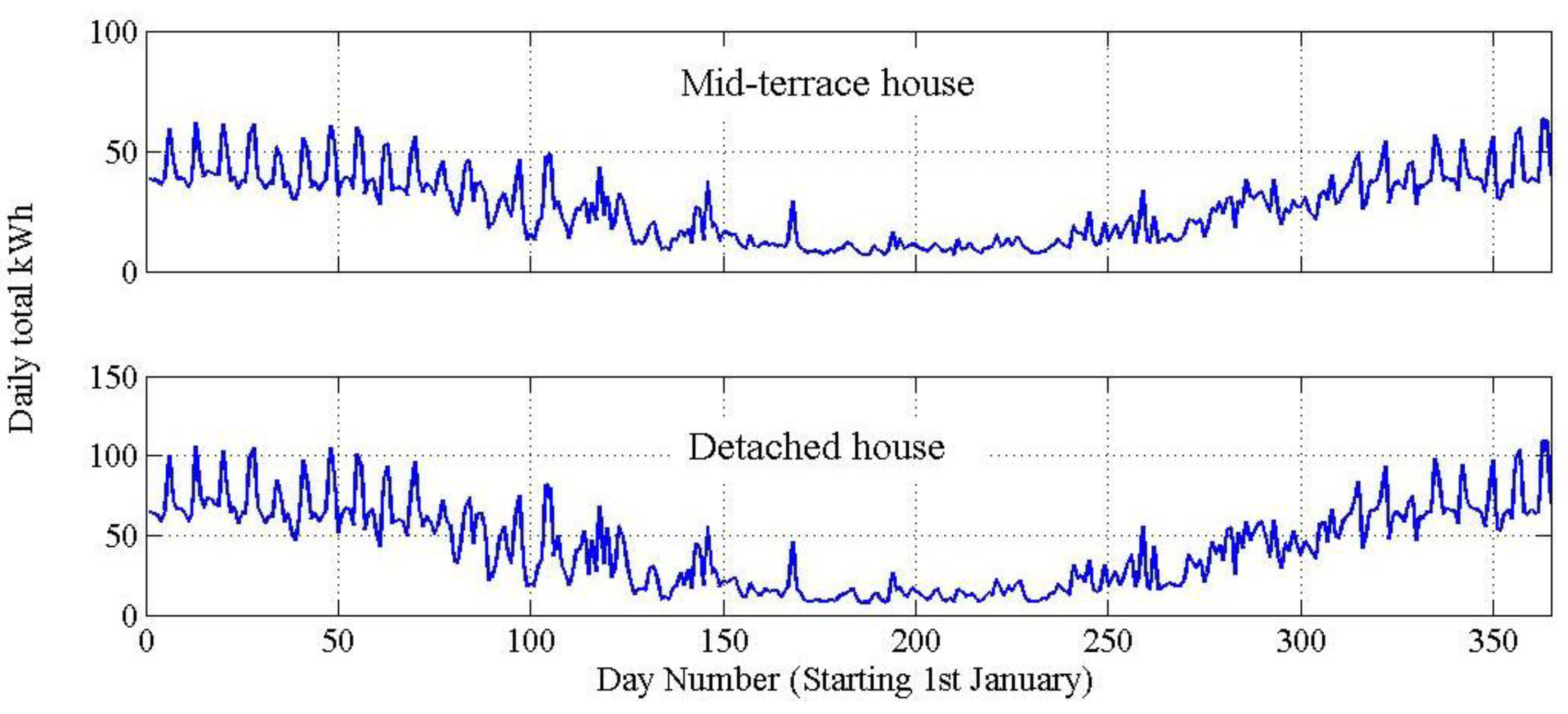
Annual total energy demands predicted using the dynamic thermal model were found to be 10,529 kWh for the mid-terrace house and 16,994 kWh for the detached house which agree very favourably with the totals from the reference model (BREDEM) given in Table 1. The annual distributions of these demands generated using the Simulink dynamic thermal model are plotted (including hot water demands) in Figure 1.
Figure 1.
Simulated distributions of energy demand due to heating and hot water.

3. Development of a Ground-Source Heat Pump Model
One of the stated objectives of this work is to take account of the decline in heat pump performance when operating at part load. Conventionally, a heat pump model capable of describing part load performance would require being fully dynamic and, consequently, very computationally demanding. A simpler model is needed particularly when the heat pump merely forms part of a more extensive modelling problem (i.e., treatment of the ground array as discussed in the next section). Historically, a simple (and conditionally accurate) modelling approach often used is the so-called “catalogue fit” model. In this, one or more dependent variables (such as electricity consumption and coefficient of performance) are fitted to a manufacturer’s performance data set using multiple-regression, e.g., [15,16,17]. These models are accurate (at least as far as that particular manufacturer’s product is concerned) but are limited in that the various standards from which these data are prepared assume static operation at the declared boundary conditions specified in the catalogue. In other words, they assume that the heat pump operates at full continuous capacity at the stated conditions. In practice, heat pumps like other energy generating plants will operate according to some control conditions and will spend large parts of the operating cycle at part load. When operating intermittently to meet a varying load under a thermostat, the first few seconds or minutes of operation as the heat pump starts is merely recovering losses prior to raising the heating temperature to a point where it can contribute to the prevailing load. Thus, in this initial phase of operation, the energy delivered by the heat pump constitutes a loss. This loss accumulates according to the number of thermostat starts the heat pump makes over a full operating cycle. Since most domestic heat pumps in use today for space heating are controlled by thermostats, losses can be significant and clearly become amplified when the heat pump capacity is larger than it needs to be (i.e., when it is over-sized). To capture this behaviour whilst also retaining a simple model structure, an empirical model is developed based on a domestic-scale laboratory pilot.
3.1. Description of the Heat Pump Test Rig
The heat pump test rig consists of a conventional domestic scale water-to-water heat pump using refrigerant R410A with a rated (nominal) heating capacity of 9.5 kW. The heat pump was controlled using a thermostat (with an adjustable set-point) mounted in the heating system return connection at the inlet to the heat pump. Detailed physical information about the heat pump can be found in Appendix C (Table C1).
The heat pump is sourced from three 100 m (deep) plus one 65 m (deep) vertical closed loop borehole heat exchangers giving a total array capacity of 365 m. All four heat exchangers are connected in parallel and each can be individually isolated to enable a variable capacity array. Each borehole heat exchanger comprises a 32 mm high density polyethylene U-tube inside a 130 mm diameter borehole with the inner spaces grouted using thermally-enhanced bentonite. The array lies in Coal Measures and a thermal response test carried out shortly after installation gave a mean soil conductivity of 2.45 W·m−1·K−1 and a borehole thermal resistance of 0.162 m·K·W−1. The undisturbed soil temperature was 12.7 °C. The source fluid is water-ethylene glycol mixture (10% ethylene glycol by volume).
The heat pump outputs to four equally-sized double panel convector-radiators which provide heating to the local laboratory environment. Each has a rated emission of 1.07 kW with reference to a mean water temperature of 40 °C and a local air temperature of 20 °C. Though the heat pump does not have a buffer tank, the heating system has a significant amount of “natural” buffering due to a low-loss header and significant runs of larger diameter (32 mm) steel piping upstream of the heating system. It is estimated that, collectively, these features provide approximately 50 L of system-side buffering that would not normally be present in a domestic installation.
Instrumentation consisted of a current clamp and voltage transducer on the incoming electrical connections to the heat pump. The power factor was measured separately using an electric circuit analyser and found to have an average value of 0.924 with very minimal variance. Source and sink heats were measured using a pair of resistance-wire temperature detectors and time-of-flight ultrasonic flow meters on both sides of the heat pump. Compound measurement uncertainties were assessed to be on average ±0.8 kW on heating loads (typically <10% of measured heat) and ±0.12 kW on active electricity use (typically <5% of measured electricity use). The laboratory air temperature was measured using several K-type thermocouples and subsequently averaged at each reporting time row.
3.2. Experimental Procedure
Forty-eight heat pump capacity tests were carried out using the following variations in plant configuration:
- 100 m, 200 m, 300 m and 365 m of source array capacity.
- 1, 2, 3 and 4 convector-radiators turned on.
- Nominal heating thermostat set point temperatures of 38 °C, 40 °C and 50 °C.
All variables were monitored at 5 s intervals and averaged in sets of six for reporting at 30 s intervals. The first and final rows of data during each on-phase were discarded in order to remove data spikes arising from incompleteness in the data during a reporting interval in which the thermostat’s status changed. Individual borehole tests were carried out on separate days to allow for soil stabilization between tests and the first thermostat cycle of results between convector-radiator adjustment events were discarded to allow for heating system stabilization. Note that the test heat pump in this case is monovalent and the logged electrical consumption includes the source pump but not the sink (heating system) pump. Thus, when used for seasonal performance evaluations, the results based on the present work would lead to a seasonal performance factor that has become referred to in some of the literature as “SPFH2” [3,8].
3.3. Results and Model-Fitting
It is well established that the performance of a heat pump depends inter alia on the source and sink temperatures. In addition, the part-load ratio (P) of the heat pump is defined here as the ratio of actual heating delivered to the maximum heating delivered. This can be determined from the results in one of two ways. Either by calculating the total heating delivered over time (in kWh) and dividing by the continuous average heating that would have been delivered over the same time period if the heat pump had not been operating intermittently; or by calculating the radiator emission from the measured heating water temperatures and laboratory air temperature. (Both methods were used and differences between them were found to be minor.)
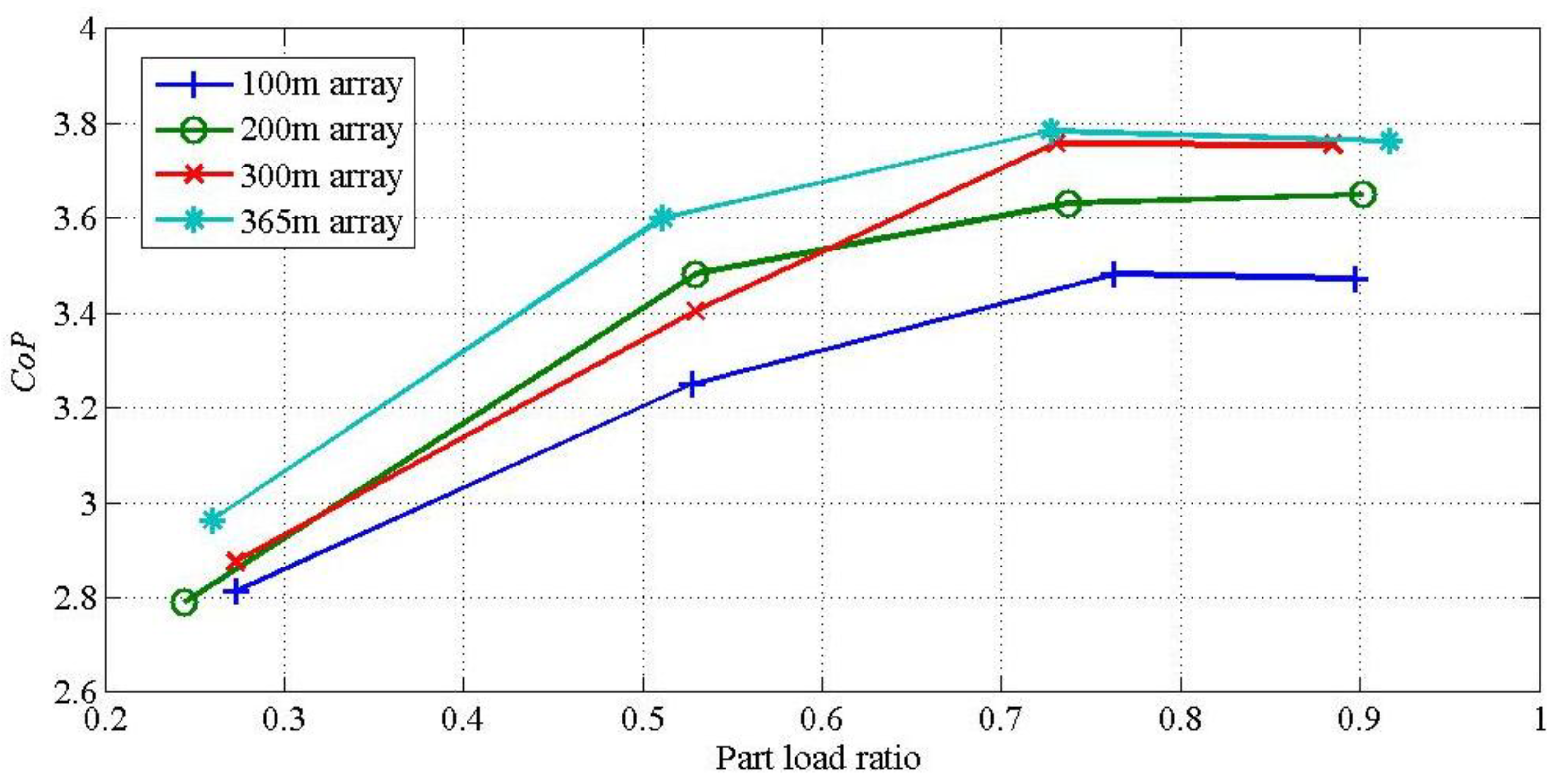
To identify the influence of the array capacity and P on the heat pump performance, each set of test results was averaged and the heat pump coefficient of performance plotted against P for each discrete array capacity. Results, given in Figure 2, show a strong influence of both of these variables on performance. It is particularly noted that the heat pump performance falls sharply at P values of ≤0.5. Therefore, the fitted model was selected to account for variations in source and sink temperature, array capacity and P. For convenience, the source and sink temperature were reduced to a temperature differential, ∆Tsosi, between heat pump outlet sink water temperature and heat pump outflow source fluid temperature. Thus, for individual fitting over each array capacity, there will be two dependent variables; P and ∆Tsosi.
Two alternative model forms were tested; bi-linear (Equation (1)) and bi-quadratic (Equation (2)):
(in which a1...d1 and a2...f2 are regression constants).
CoP = (a1 + b1 × P) × (c1 + d1 × ∆Tsosi)
CoP = (a2 + b2 × P + c2 × P2) × (d2 + e2 × ∆Tsosi + f2 × ∆Tsosi2)
Figure 2.
Part load performance results from the heat pump test rig.

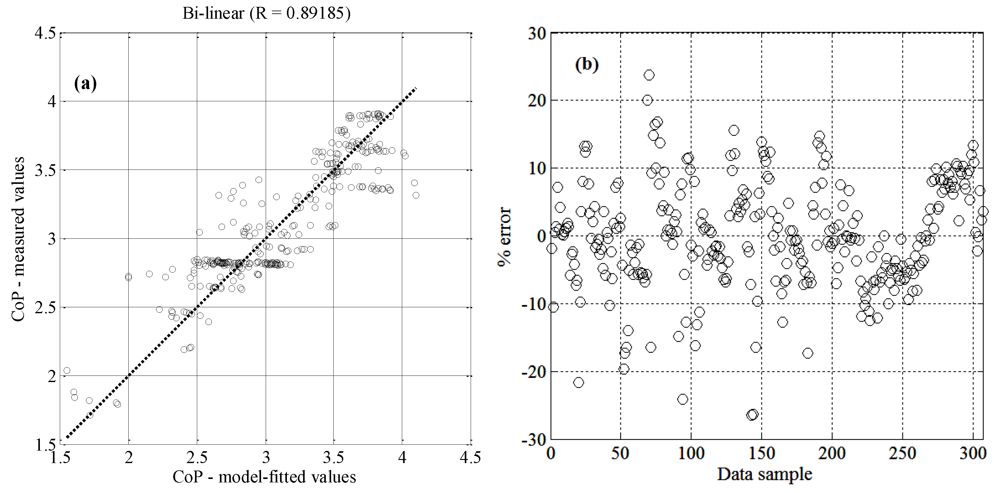
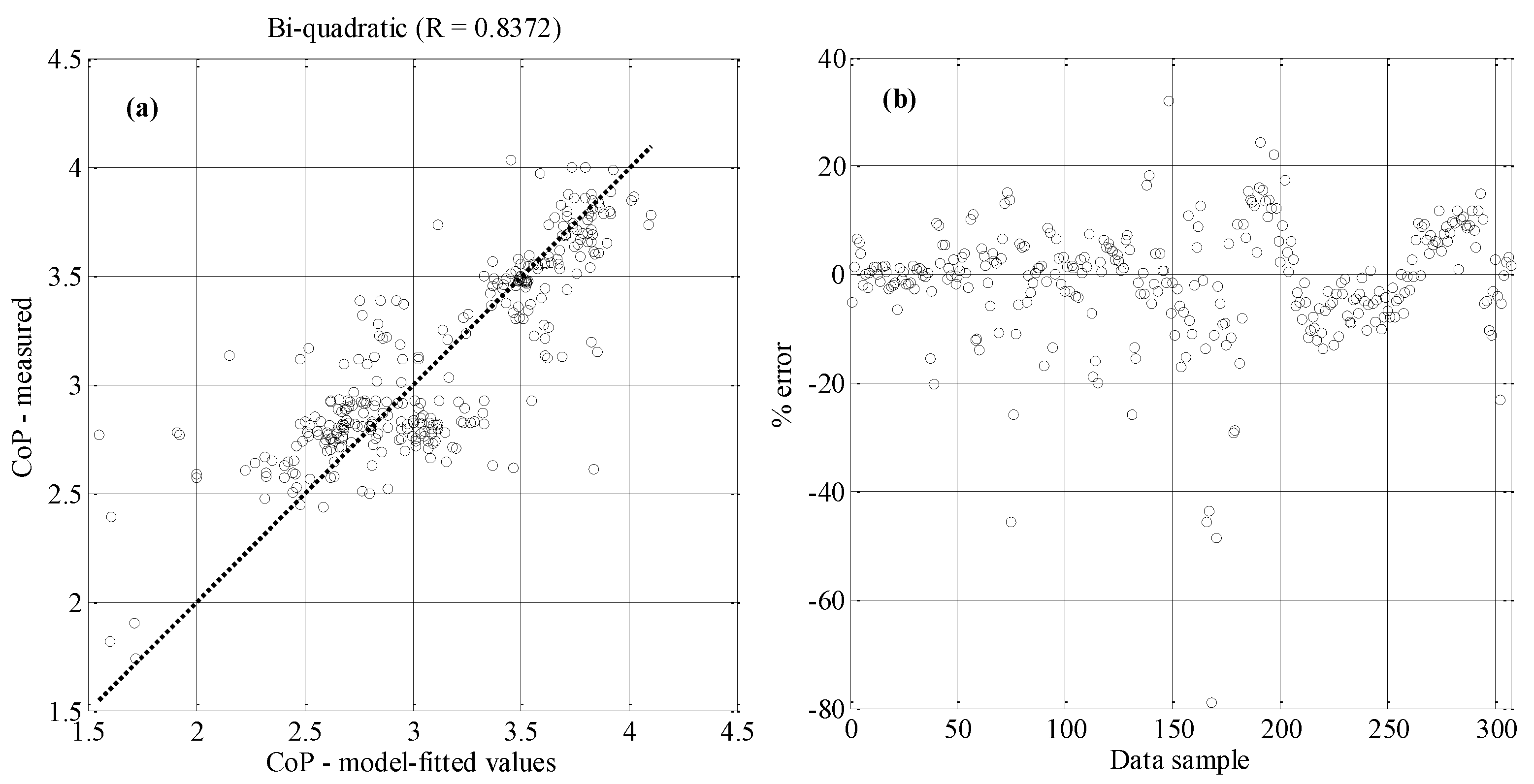
Results of multiple-regression fitting over all viable data using both models are summarized in Figure 3 and Figure 4. For the bi-linear model, most of the target/model error values across all data are within ±10%. There is no improvement in goodness-of-fit when adopting the slightly more complex bi-quadratic model and the target/model error values here are mostly contained within the higher error range of ±20%. Hence, the bi-linear model is adopted in this work. Multiplying out Equation (1) gives the following for which values of the fitted constants, A, B, C, and D, for all array capacities investigated can be found in Table 2:
CoP = A + B × P + C × ∆Tsosi + D × P × ∆Tsosi
Figure 3.
Bi-linear model fitting results. (a): Regression plot; (b): Target-model errors (%).

Figure 4.
Bi-quadratic model fitting results. (a): Regression plot; (b): Target-model errors (%).

| Array Size (m) | A | B | C | D |
|---|---|---|---|---|
| 100 | 2.852525 | 2.868282 | −0.017015 | −0.037951 |
| 200 | 7.936727 | −1.206375 | −0.154520 | 0.067780 |
| 300 | 3.315421 | 2.816345 | −0.021494 | −0.042534 |
| 365 | 3.188746 | 3.414232 | −0.017961 | −0.062144 |
4. Ground Array Modelling
The closed loop vertical array was modelled as a conventional heat exchanger problem using Kays and London’s classical “number of transfer units” (NTU) method [18]. This involved calculating the number of heat exchange transfer units from which the array effectiveness could be determined (Equations (4) and (5)):
![Energies 07 04532 i001]()

Earray = 1 − exp(−NTU)
Note that the specific heat capacity of the array fluid, cpf,array, is calculated using the properties of ethylene glycol solution at the user-defined ethylene glycol concentration. In the present work, the concentration was set at 20% (by volume). The heat exchange (i.e., array) effectiveness is defined as the heat transfer achieved divided by the maximum theoretically possible heat transfer. Thus, the array outlet temperature can be calculated at each time row in the simulation from Equation (6):
(where Tarray,soil is the current time row average of the soil temperature along the paths of the array heat exchangers).
Tf,array,out = Tarray,soil + ∆Tf,max × (1 − 1/Earray)
For the soil domain, a three-dimensional (in space) dynamic numerical solution of the Energy Equation was used through a uniformly discretized grid cast throughout a defined soil domain. Full details of this model can be found in [19]. The house time-series energy demands described in Section 2.2 are read into this model and used to calculate the energy balance on the new heat pump model described in Section 3.3 and the array model described above. This leads to a heat pump source flux at each time row which is then uniformly imposed on the defined array path in the soil domain model. In effect, this amounts to imposing a variable line source of heat on the numerical soil domain model.
The soil domain model used a 50 m × 50 m × 150 m (deep) domain size with a uniform 1 m grid mesh size. The grid mesh size was found to be acceptable for long time horizon simulations (such as in the present work) but a smaller size is needed for short-time simulations (a further discussion about this can be found in [19]). The domain size was found to give good results for up to 5 years of simulation duration. A comparison with a 100 m × 100 m × 150 m domain size was made and differences in results in the key variable of heat pump electricity usage were found to be negligible (the larger domain requiring almost five-times the computation effort as the smaller domain). A uniform undisturbed earth temperature distribution (see Section 5) was imposed throughout the domain as an initial condition and the boundaries of the domain were held at these values. A uniform time step of 1 h was used. The computation time on a quad-core workstation was found to be 4.7 h of simulation time per 1 s of computer elapsed time. The entire ground, heat pump and array model was implemented as a bespoke Matlab function.
5. Results and Discussion
Reviews of soil properties based on thermal response tests carried out in the UK have received attention recently. Underwood [19] reported on 13 such tests from a variety of sites giving lower quartile, median and upper quartile soil thermal conductivities of 2.40 W·m−1·K−1, 2.47 W·m−1·K−1 and 3.08 W·m−1·K−1, respectively and lower quartile, median and upper quartile borehole resistances of 0.152 m·K·W−1, 0.162 m·K·W−1 and 0.216 m·K·W−1, respectively. Banks et al. [20] reported on a much larger sample of 61 UK sites. Correspondingly, conductivities were found to be 1.86 W·m−1·K−1, 2.25 W·m−1·K−1 and 3.00 W·m−1·K−1, respectively, and borehole thermal resistances of 0.09 m·K·W−1, 0.11 m·K·W−1 and 0.14 m·K·W−1, respectively [20]. There are some similarities in the conductivity results between the two sources though there are differences between borehole resistance values most likely due to different methods being used to arrive at the results from basic measurements (extraction using a bespoke optimisation algorithm in [19] and extraction by conventional line source theory in [20]). Since [20] represents the larger sample of data, these results will be used in the evaluative modelling that follows. In addition, the undisturbed ground temperatures at the lower quartile, median and upper quartile of 11.7 °C, 12.3 °C and 13.2 °C [20] are used.
5.1. Array Design
The median soil property and borehole resistance data reported in [20] were used for initial array design:
| Soil thermal conductivity: | 2.25 W·m−1·K−1 |
| Borehole thermal resistance: | 0.11 m·K·W−1 |
| Undisturbed soil temperature: | 12.3 °C |
In addition, the volume heat capacity for the soil was assumed to be 2.4 MJ·m−3·K−1 which is appropriate for a wide range of soil and rock types. Reference is made to the house design heat losses detailed in Appendix A, Table A2; a notional design coefficient of performance of 2.82 as suggested by the Energy Saving Trust’s most recent field trials [3]; and the array design look-up tables contained in the Microgeneration Certification Scheme (MCS) [2]. Using this information, recommended array designs of 83 m for the mid-terrace house and 138 m for the detached house were arrived at. These array sizes would therefore be used in normal practice.
For design evaluation, simulations using the foregoing data together with the time-series energy demands detailed in Section 2.2 were carried out for both house types based on a range of array sizes starting with the MCS values of 83 m and 138 m for the respective house types. Results in the form of alternative heat pump seasonal performance factors (SPF) are summarized in Table 3. Note that seasonal performance factors used in the present work are what have become referred to in some of the literature as “SPFH2” [3,8]. They are applicable to a monovalent heat pump (including source fluid pump) electricity use but exclude the heating system (sink) pump. For all simulations, the heat pump heating water outlet temperature set point was fixed at 42 °C which is within the range of the test results described in Section 3.2 upon which the heat pump model is based. It was assumed that all space heating and domestic hot water loads are delivered at this temperature from the heat pump buffer store of capacity 50 L. No allowance has been made in the present work for additional direct electric heating due to periodic hot water pasteurization (if used).
| Array Size (m) | Mid-Terrace House | Detached House | ||
|---|---|---|---|---|
| SPF | Improvement | SPF | Improvement | |
| 83 (MCS, [2]) | 3.05 | - | - | - |
| 138 (MCS, [2]) | - | - | 3.02 | - |
| 200 | 3.32 | 8.9% | 3.14 | 4.0% |
| 300 | 3.38 | 1.8% | 3.33 | 6.1% |
| 400 | 3.35 | - | 3.31 | - |
Comments: The performances based on array sizes recommended by the MCS are broadly consistent with the median performance of the actual installations monitored by the Energy Saving Trust [3] after improvements had been made (i.e., 3.1). For both house types, there are improvements of up to around 10% in the heat pump SPF by increasing the array size significantly. For the mid-terrace house, increasing the array size by a little over 100 m beyond the value recommended by the MCS gives a performance improvement of 8.9% whereas a further increase by 100 m results in a much lower improvement of 1.8% and there is no improvement at higher array sizes. Therefore, a design array size of 200 m would seem appropriate for this case. For the detached house, there is a performance improvement of 4% when increasing from the MCS recommended array size to 200 m and the improvement increases to 6.1% when increasing from 200–300 m after which there is no further improvement with increasing array size. Thus, a 300 m array would seem to be the appropriate choice here.
In the subsequent analyses, the array size for the mid-terrace house will be set at 200 m and, for the detached house, 300 m.
5.2. Sensitivity to Time Horizon
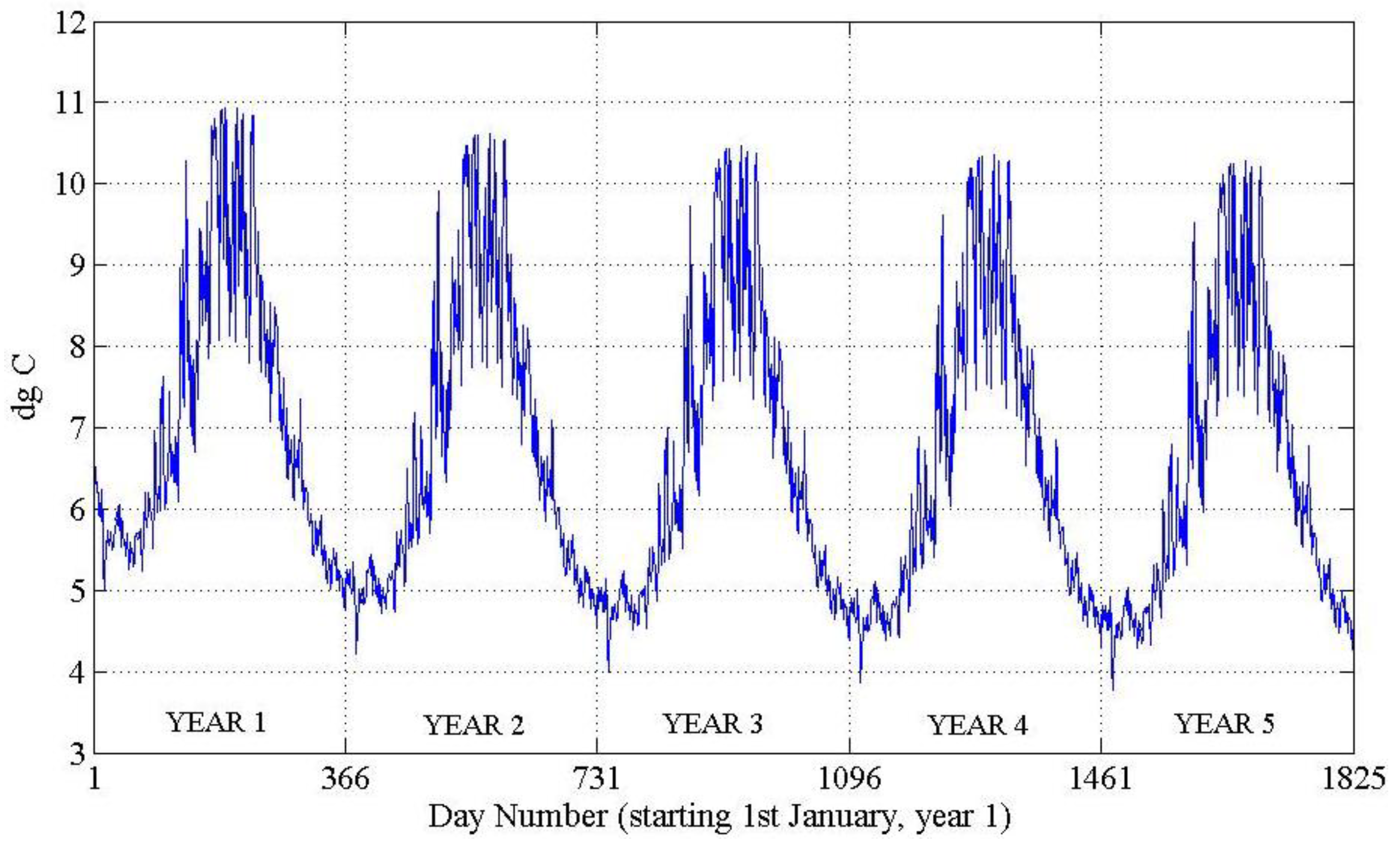
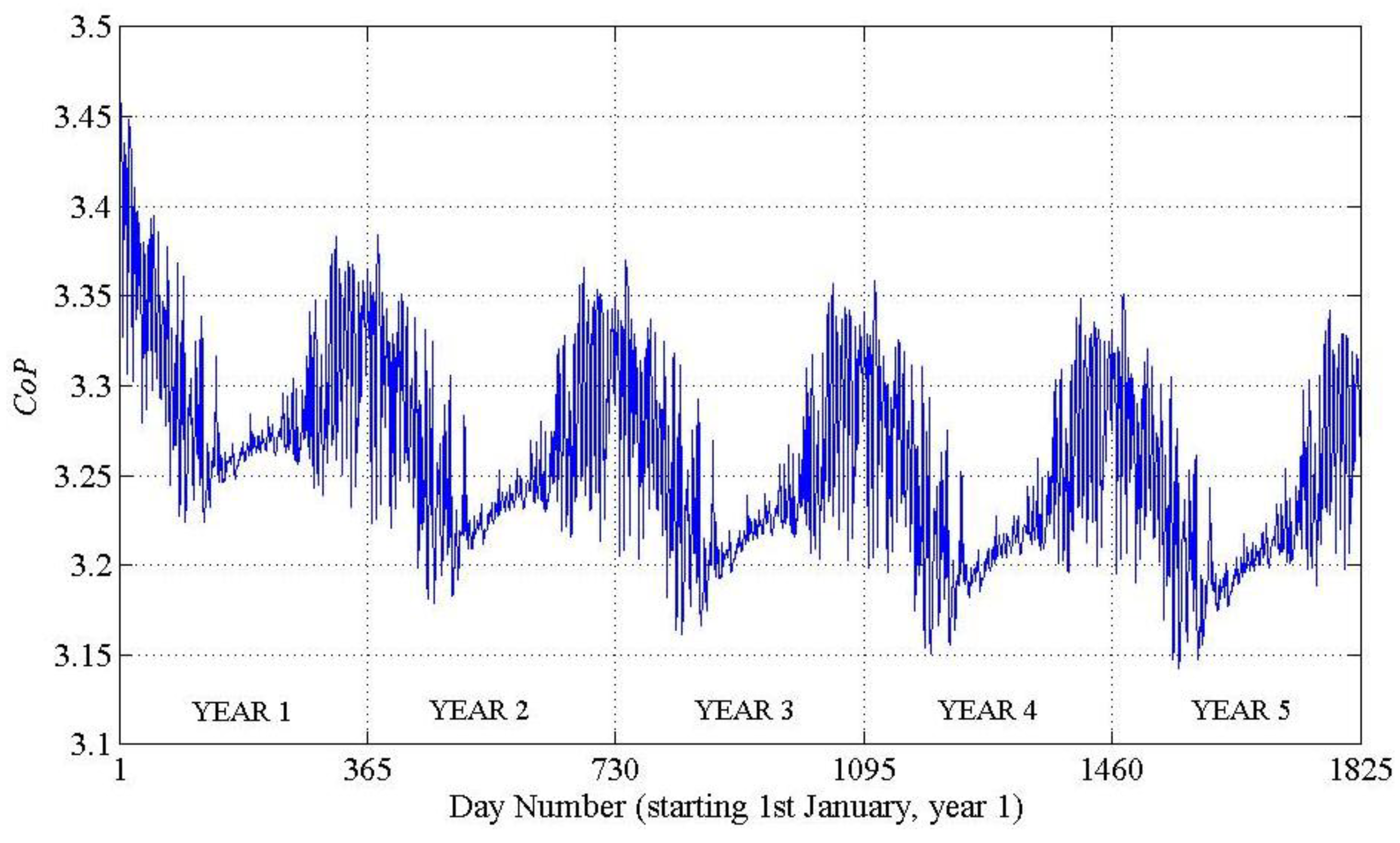
To test the designs over an extended operating period, the array sizes and other design conditions set out in Section 5.1 were applied to five-year simulations for each house. It was assumed that the annual demand patterns (Figure 1) remained the same in each year. Results of the daily minimum array inlet temperatures over the five-year duration are provided in Figure 5 and Figure 6 for both houses. Results of the daily mean heat pump coefficient of performance over the same duration are given in Figure 7 and Figure 8 also for both houses.
Comments: As is to be expected, there is a decline in minimum array fluid temperature over the extended operating time horizon though the rate of decline reduces over time particularly after the first year. What is important with these array designs is that the array fluid temperature for both houses barely falls below 4 °C which suggests that fresh water (rather than ethylene glycol solution) might safely be used with corresponding performance, cost and environmental advantages. The trends in heat pump coefficient of performance (Figure 7 and Figure 8) show a small decline over the five-year period as the ground temperature reduces and a more pronounced decline in the middle period of each year. This is because light loads are being met at these times (i.e., domestic hot water only) with the consequence that the heat pump is operating highly intermittently. (A key assumption in the modelling is that the thermostatically-controlled heat pump operates at the same set point temperature (42 °C) at all times for both heating and hot water delivery and so the heat pump performance is governed by intermittent operation and seasonal variations in the source temperature.) Equally, though the performance is inferior at this time of the year, the heating delivered (and therefore electrical energy consumed by the heat pump) will be lower than in winter and this mitigates the inferior heat pump performance to some extent. The decline in heat pump performance over the five-year horizon is more pronounced with the mid-terrace house than with the detached house and the detached house exhibits a more pronounced dip in summer heat pump performance. The reason for this is that the domestic hot water loads are similar for both houses whereas the detached house has a significantly higher heat load due to space heating. The correspondingly larger array size for the detached house recovers better in summer when demands are light than the mid-terrace house which has the smaller array size. However, a lower pattern of P for the detached house due to higher heat load but only marginal increases in summer hot water load results in a lower summer CoP than experienced by the mid-terrace house. Again, because relatively low amounts of energy are generated in summer, the inferior heat pump performance is mitigated to some extent.
Figure 5.
Minimum daily array inlet temperatures (mid-terrace house).

Figure 6.
Minimum daily array inlet temperatures (detached house).

Figure 7.
Mean daily heat pump CoP (mid-terrace house).

Figure 8.
Mean daily heat pump CoP (detached house).

5.3. Sensitivity to Soil Conductivity and Array Resistance
To evaluate the sensitivity of the designs to variations in soil conductivity and borehole heat exchanger resistance values, a simulation was conducted using alternative soil conductivities of 1.86 W·m−1·K−1 (i.e., the lower quartile value from the Banks et al. review [20]) and a further simulation was conducted using this lower conductivity and a higher borehole resistance value of 0.216 m·K·W−1. In the choice of the latter value, the upper quartile resistance from [19] was used instead of from [20] since the range of values in [19] was wider. Results of the original seasonal performance factors compared with the new values arising from these changes in soil and borehole properties are given in Table 4.
Comments: The results show that the performance is not significantly affected by a “typical” range of soil and resistance properties found in UK conditions. Here, the results appear to be more sensitive to borehole resistance than soil conductivity though it should be stressed that this illustration involved a relatively minor reduction in conductivity and a substantial (near doubling) increase in borehole resistance. However, it is becoming clear that the range of soil conductivities across many UK applications is relatively low and this prompts the need to consider carefully whether expensive thermal response testing is needed in every case when ground geology is known with a reasonable degree of confidence. It should also be pointed out that, in most cases, the existence of groundwater flows (not considered in this work) will actually improve performance.
| Property Choices | SPF | |
|---|---|---|
| Mid-Terrace House | Detached House | |
| Median (design) values | 3.32 | 3.33 |
| Reduced k | 3.31 | 3.33 |
| Reduced k & increased Rbhx | 3.17 | 3.26 |
5.4. Sensitivity to Heating System Sizing
A final analysis was carried out into the impact of heating system sizing. First, the simulation was re-run with P (in Equation (3)) fixed at a constant value of 1. This will show how much additional energy is required due to the deleterious part-load performance of the heat pump thus revealing the potential for improved control over the heat pump at light loads. Second, the simulation was re-run for both houses with the heating system capacity (Table A2, Appendix A) reduced by 20%, and then increased by 20% and 40%.
Results, compared with the original design results for reference, are given in Table 5. Also included are the averages of the comfort (operative) temperature of the whole house averaged over all periods when the space heating system is active only. Note that the operative temperature as used here is the average of the internal air and mean radiant temperatures.
| Capacity Options | Mid-Terrace House | Detached House | ||||
|---|---|---|---|---|---|---|
| SPF | kWh·m−2 | TOP (°C) | SPF | kWh·m−2 | TOP (°C) | |
| Perfect tracking | 3.56 | 36.1 | 19.97 | 3.75 | 33.0 | 19.74 |
| Design | 3.32 | 38.6 | 19.97 | 3.33 | 37.1 | 19.74 |
| 20% under-sizing | 3.34 | 35.9 | 18.68 | 3.35 | 34.5 | 18.46 |
| 20% over-sizing | 3.31 | 40.8 | 20.61 | 3.31 | 38.9 | 20.54 |
| 40% over-sizing | 3.30 | 42.4 | 21.19 | 3.29 | 40.3 | 21.04 |
(kWh·m−2: annual electricity usage due to heat pump and source fluid pump divided by house gross floor area).
Comments: A 40% heating system over-sizing margin will not translate to a 40% increase in energy because the heating system controls will act to regulate the system to the required comfort conditions. However, oversizing will lead to an increase in energy because an over-sized control system will not be able to track the required control condition perfectly. In particular, the use of simple proportional controls used in domestic “thermostatic” radiator valves will exhibit offset (a sustained difference between set point and actual value). Thus, an over-sized system will lead to an increase in both energy use and comfort temperature. Consequently, the seasonal performance factor is not significantly affected by over-sizing (or under-sizing), however the electricity consumed has increased in all over-sizing cases. If the heat pump was able to operate over all load patterns without loss in performance it would operate with a SPF in excess of 3.5 for both houses. This falls to around 3.3 for both houses when its part load behavior is accounted for and the electrical consumption increases by 7% (mid-terrace house) and 12% (detached). If the heating is oversized by up to 40% the energy consumption over a heat pump well matched to the load at all times will increase by almost 18% (mid-terrace house) and 22% (detached house). These should be considered as viable targets for further improvements in domestic heat pump performances in the UK where evidence of equipment over-sizing is plentiful. A particularly notable result in Table 5 is revealed that when the heating system is under-sized by 20% the energy use falls whilst comfort remains very close to acceptable limits. Note here that the area-weighted target comfort temperature for both houses based on 21 °C in the main living space and 18 °C in all other spaces is 18.5 °C—almost precisely met on average by a heating system that is under-sized by 20%. The reason for this is that conventional heating sizing is carried out using steady-state calculations at boundary conditions that, in many winters, will never be realized or if they are, will be of short duration. There is a compelling case for the use of dynamic thermal modelling for the sizing of complex systems such as heat pumps and other microgenerators.
6. Conclusions
The aim of this work was to investigate the impact of heat pump capacity and ground array design for domestic ground source heat pumps operating in UK conditions with a view to establishing design criteria that might lead to improvements in operating performance.
The work has been largely based on numerical modelling supported with the introduction of a new empirical heat pump model which takes into account the decline in heat pump performance during periods of light load. Results have been drawn from two exemplar houses which have been configured to be typical of common terraced and detached houses in the UK and use has been made of an existing numerical model of a closed loop vertical ground array.
The results of this work suggest vertical ground loop array sizes for the two typical house types investigated of around 2.5 m of array length per m2 of house gross floor area. The recommended allowance using the Microgeneration Certification Scheme recommendations would be around 1.1 m/m2. Furthermore, the array sizes proposed in this work show that it will be possible to operate the array safely using fresh water rather than ethylene glycol solution (or some other form of antifreeze) which is beneficial for performance, cost and the environment.
As data on ground thermal conductivities in the UK start to become more abundant, it is becoming clear that many sites have mean conductivities of around 2–2.5 W·m−1·K−1 and modest variations about this figure have little effect on heat pump performance. However, the more uncertain values of borehole heat exchanger resistance do have an influence on performance.
The impact of both deteriorating part-load performance of thermostatically-controlled ground source heat pumps and heating system over-sizing (by up to 40%) has been shown to increase energy use by up to 18%–22% for the two typical house types considered.
Evidence in this work points to a strong potential for a better matching of the capacity of ground source heat pumps to the required building load pattern through the use of dynamic thermal modelling instead of conventional steady-state design methods.
Further work is needed in the following areas:
- Development of verifiably accurate and easy-to-use tools for the design and seasonal performance evaluation of ground source heat pumps suitable for use by practitioners.
- Consideration of the impact of groundwater flow over closed loop arrays in UK conditions.
- Investigations into variable speed drives, electronic expansion devices and improved controls for domestic scale heat pumps.
- Development of alternative dynamically-based methods for system design and capacity-sizing as an alternative to conventional steady-state sizing methods.
Glossary
| a1...d1 | Regression constants |
| a2...f2 | Regression constants |
| A...D | Regression constants |
| CoP | Coefficient of performance (dimensionless)—instantaneous or short-time average heat output divided by instantaneous or short-time average heat pump plus source fluid pump electrical consumption |
| cpf,array | Specific heat capacity of array fluid (J·kg−1·K−1) |
| Earray | Array (heat transfer) effectiveness |
| k | Soil mean thermal conductivity (W·m−1·K−1) |
| Larray | Total array length (m) |
| mf,array | Array fluid mass flow rate (kg·s−1) |
| NTUarray | Array number of (heat) transfer units |
| P | Part load ratio (current heating demand divided by seasonal maximum heating demand) |
| R | Correlation coefficient |
| SPF | Seasonal performance factor (dimensionless)—seasonal heat pump heating energy divided by seasonal heat pump plus source fluid pump electrical consumption |
| Rbhx | Borehole heat exchanger thermal resistance (m·K·W−1) |
| Tf,array,out | Array fluid outlet temperature (°C) |
| Tarray,soil | Average soil temperature along the entire array path (°C) |
| TOP | Room space operative temperature (°C) |
| ∆Tf,max | Maximum (design) array inlet/outlet fluid temperature difference (K) |
| ∆Tsosi | Heat pump nominal temperature lift (difference between the heating outlet temperature (K or °C) and the source fluid outlet temperature (K or °C) |
Symbols used in Table A1 and Table A2
| MT | mid-terrace |
| DET | detached |
| GFA | gross floor area |
| LS | main living space |
| B | balance of ground floor space |
| FF | first floor |
Appendix A. Seasonal Energy Demand Modelling
| Type | Areas (m2) | Footprint | Orientation | Windows | Glazing (m2 *) | Roof | ||
|---|---|---|---|---|---|---|---|---|
| GFA | LS | Width (m) | Depth (m) | |||||
| MT | 75 | 12 | 6.1 | 6.1 | N-S | Clear double | 10.4 | Pitched |
| DET | 125 | 20 | 7.9 | 7.9 | N-S | Clear double | 17.2 | Pitched |
* Based on the UK Standard Assessment Procedure: 0.1382 × GFA − 0.027. An additional allowance of one single door (rear) and one single door (front) of 2 m2 (each) is added to the window areas.
| U-values (W·m2·K−1) | Design Temperatures (°C) | Ventilation (h−1) | Design Loss (kW *) | |||||
|---|---|---|---|---|---|---|---|---|
| Wall | Roof | Gr-floor | Window | LS | B | FF | ||
| 0.45 | 0.35 | 0.45 | 2.2 | 21 | 18 | 18 | 0.5 | 3.09 |
| 0.45 | 0.35 | 0.45 | 2.2 | 21 | 18 | 18 | 0.5 | 5.95 |
* Design heat loss with an external design temperature of −3 °C. Calculations include a pre-heat margin of 25% and were carried out in accordance with the methods set out in the CIBSE Guide. The standards are those that would be expected of UK houses either constructed or refurbished at around 2002.
Appendix B. Dynamic Thermal Modelling—Simulink HVAC Blockset
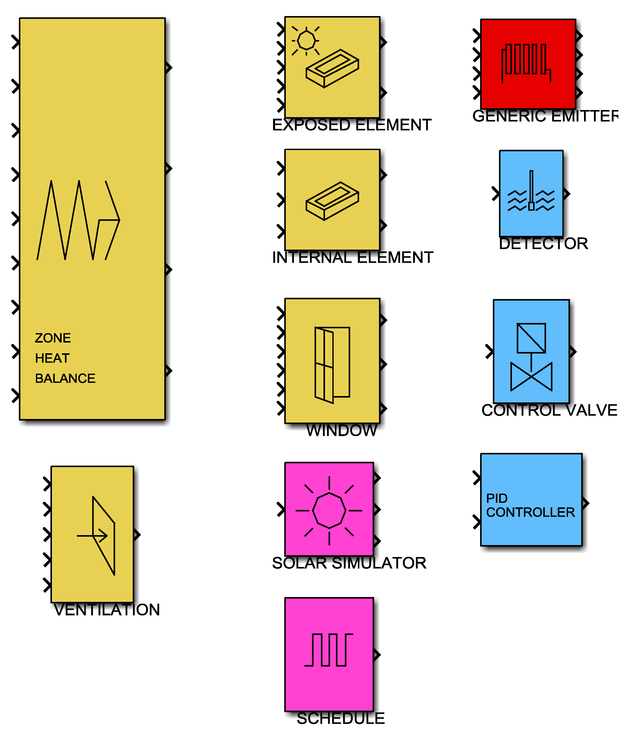
The Simulink HVAC Blockset is a generic Simulink library that can be used to construct detailed dynamic models of buildings including HVAC plant and controls and certain embedded renewable energy systems. Several such libraries exist for modelling energy in buildings such as SIMBAD [21] and CARNOT [22] but the advantage of the HVAC Blockset used here is that all component models are fully dynamic, enabling more accurate control and system response modelling to be carried out. (The HVAC Blockset used here is made freely available by the author for other users.) Note that only certain component model selections were used in the present work as detailed below.
Components used to remodel the two house types:
| Building envelope: | Plant and controls: | Utility: |
| Zone heat balance | Generic emitter 2 | Schedule 4 |
| Exposed element | Detector 3 | Solar simulator 5 |
| Internal element | Control valve 3 | |
| Window | PID controller 3 | |
| Ventilation 1 |
- Infiltration due to wind and stack effect during winter with closed windows. The block was set to open windows by 50% of their opening capacity when internal temperatures reached 26 °C and by a further 50% to fully-open when temperatures reached 28 °C (i.e., in summer when the heating is off).
- The “generic emitter” was used to represent panel convector-radiator heating.
- The “detector”, “control valve” and “PID controller” blocks were combined to represent “thermostatic” radiators valves attached to each zone radiator. Only the proportional term of the PID controller block was enacted. The detector was set with a long time constant (3 min) to help represent the long time delay in these valves. (Note that the widely-used term “thermostatic” is a misnomer in this context since these control valves actually modulate the hot water flow rate in practice.)
- Separate “schedule” blocks were used to represent switching of occupant activity and plant activity.
- The “solar simulator” was used to generate in-plane irradiances on each exposed window and opaque surface.
Figure B1.
Simulink HVAC Blockset.

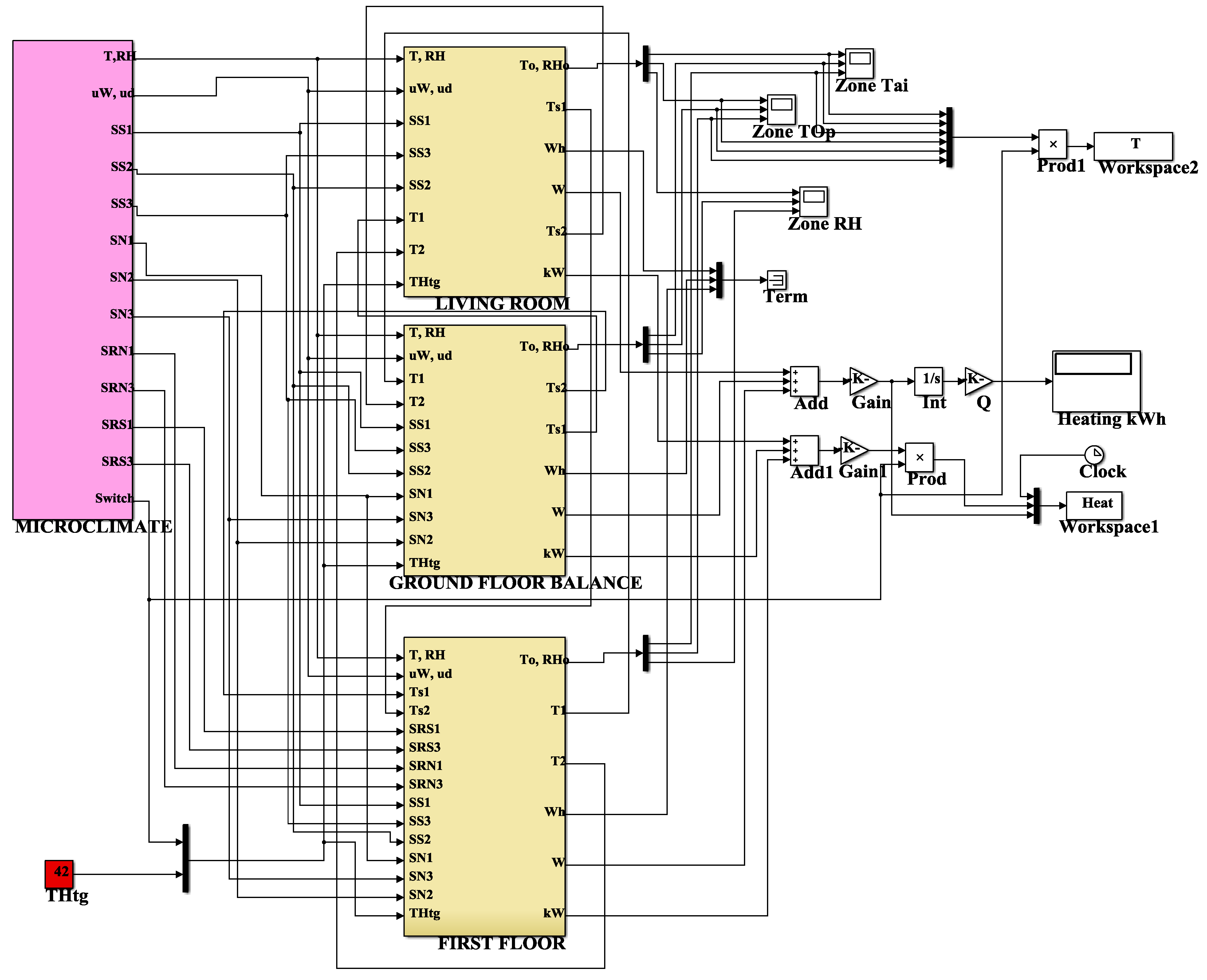
The highest level of the Simulink model created for the mid-terrace house is shown as an example in Figure B2, showing all parent blocks and information flows between them. The three main blocks at the centre represent the parent blocks of the living room (top), balance of ground floor spaces (middle) and first floor (bottom). Beneath these parent blocks are all the component blocks (and their information flow connections) for the room elements, zone energy balance, ventilation, heating system and heating controls. The large block to the left in Figure B2 is the parent block which contains all microclimate modelling (i.e., a file-read utility which reads in weather data and solar simulating blocks for all orientations forming the mid-terrace house).
Note that the other blocks shown in the generic library and not specifically referred to above were not used in the present work. Furthermore, the heat pump model in the generic library (which is a simple manufacturer’s catalogue-fit type model) was not used in the present work either.
Figure B2.
Top-level block diagram model for the mid-terrace house.

Appendix C. Details of the Test Ground Source Heat Pump
| System Component | Parameter | Value |
|---|---|---|
| Compressor | Type | Scroll |
| Refrigerant | R410A | |
| Electrical supply | 1-phase, 220 V | |
| Displacement | 5.34 m3·h−1 | |
| Evaporator and condenser | Type | Brazed plate |
| Plate material | Corrugated stainless steel | |
| Number of plates | 13 | |
| Plate width | 118.4 mm | |
| Plate height | 440 mm | |
| Plate spacing | 2.24 mm | |
| Plate thickness | 0.4 mm | |
| Volume, refrigerant side | 0.57 L | |
| Volume, water side | 0.66 L | |
| Expansion device | Type | Mechanical, thermostatic |
Conflicts of Interest
The author declares no conflict of interest.
References
- Getting Warmer: A Field Trial of Heat Pumps. Available online: http://www.heatpumps.org.uk/PdfFiles/TheEnergySavingTrust-GettingWarmerAFieldTrialOfHeatPumps.pdf (accessed on 11 December 2013).
- Microgeneration Installation Standard MIS 3005—Requirements for Contractors Undertaking the Supply, Design, Installation, Set to Work, Commissioning and Handover of Microgeneration Heat Pump Systems, Issue 4.0. Available online: http://www.microgenerationcertification.org/images/MIS%203005%20Issue%204.0%20Heat%20Pump%20Systems%20%202013.12.16%20FINAL3.pdf (accessed on 25 April 2014).
- The Heat is on. Available online: http://www.energysavingtrust.org.uk/Organisations/Technology/Field-trials-and-monitoring/Fieldmonitoring/Field-trial-reports/Heat-pump-field-trials (accessed on 25 April 2014).
- Bagdanavicius, A.; Jenkins, N. Power requirements of ground source heat pumps in a residential area. Appl. Energy 2013, 101, 591–600. [Google Scholar] [CrossRef]
- Blanco, D.L.; Nagano, K.; Morimoto, M. Experimental study on a monovalent inverter-driven water-to-water heat pump with a desuperheater for low energy houses. Appl. Therm. Eng. 2013, 50, 826–836. [Google Scholar] [CrossRef]
- Wood, C.J.; Liu, H.; Riffat, S.B. An investigation of the heat pump performance and ground temperature of a pile foundation heat exchanger system for a residential building. Energy 2010, 35, 4932–4940. [Google Scholar]
- Boait, P.J.; Fan, D.; Stafford, A. Performance and control of domestic ground-source heat pumps in retrofit installations. Energy Build. 2011, 43, 1968–1976. [Google Scholar] [CrossRef]
- Gleeson, C.P.; Lowe, R. Meta-analysis of European heat pump field trial efficiencies. Energy Build. 2013, 66, 637–647. [Google Scholar] [CrossRef]
- Fernández-Seara, J.; Pereiro, A.; Bastos, S.; Dopazo, J.A. Experimental evaluation of a geothermal heat pump for space heating and domestic water simultaneous production. Renew. Energy 2012, 48, 482–488. [Google Scholar] [CrossRef]
- National Energy Efficiency Data-Framework (NEED), Table 1. Available online: https://www.gov.uk/government/collections/national-energy-efficiency-data-need-framework (accessed on 28 April 2014).
- BREDEM 2010—A Technical Description of the BRE Domestic Energy Model, Version 1.0. Available online: http://www.bre.co.uk/filelibrary/bredem/BREDEM-2012-specification.pdf (accessed on 28 April 2014).
- Gouda, M.M.; Danaher, S.; Underwood, C.P. Building thermal model reduction using nonlinear constrained optimization. Build. Environ. 2002, 37, 1255–1265. [Google Scholar] [CrossRef]
- Gouda, M.M.; Underwood, C.P.; Danaher, S. Modelling the robustness properties of HVAC plant under feedback control. Build. Serv. Eng. Res. Technol. 2003, 24, 271–280. [Google Scholar]
- CIBSE TM48. Use of Climate Change Scenarios for Building Simulation: The CIBSE Future Weather Years; Chartered Institution of Building Services Engineers: London, UK, 2009. [Google Scholar]
- Underwood, C.P.; Yik, F.W.H. Modelling Methods for Energy in Buildings; Blackwell: Oxford, UK, Chapter 4; 2004; pp. 135–137. [Google Scholar]
- Fisher, D.E.; Rees, S.J.; Padhmanabhan, S.K.; Murugappan, A. Integration and validation of ground source heat pump system models in an integrated building and system simulation environment. HVAC&R Res. 2006, 12, 693–710. [Google Scholar]
- Kinab, E.; Marchio, D.; Rivière, P.; Zonghaib, A. Reversible heat pump model for seasonal performance optimization. Energy Build. 2010, 42, 2269–2280. [Google Scholar] [CrossRef]
- Kays, W.M.; London, A.L. Compact Heat Exchangers, 2nd ed.; McGraw-Hill: New York, NY, USA, 1964. [Google Scholar]
- Underwood, C.P. Ground-source heat pumps: Observations from United Kingdom ground thermal response tests. Build. Serv. Eng. Res. Technol. 2013, 34, 123–144. [Google Scholar] [CrossRef]
- Banks, D.; Withers, J.G.; Cashmore, G.; Dimelow, C. An overview of the results of 61 in situ thermal response tests in the UK. Q. J. Eng. Geol. Hydrogeol. 2013, 46, 281–291. [Google Scholar]
- SIMBAD—Simulation of Buildings and Devices. Available online: http://www.simbad-cstb.fr/ (accessed on 20 June 2014).
- CARNOT—Conventional and Renewable Energy Siystems Optimisation Blockset. Available online: http://mv.fh-duesseldorf.de/d_pers/Adam_Mario/a_lehre/gm_allg_down/Carnot-Hilfe.pdf (accessed on 20 June 2014).
© 2014 by the authors; licensee MDPI, Basel, Switzerland. This article is an open access article distributed under the terms and conditions of the Creative Commons Attribution license (http://creativecommons.org/licenses/by/3.0/).
Share and Cite
MDPI and ACS Style
Underwood, C. On the Design and Response of Domestic Ground-Source Heat Pumps in the UK. Energies 2014, 7, 4532-4553. https://doi.org/10.3390/en7074532
AMA Style
Underwood C. On the Design and Response of Domestic Ground-Source Heat Pumps in the UK. Energies. 2014; 7(7):4532-4553. https://doi.org/10.3390/en7074532
Chicago/Turabian StyleUnderwood, Chris. 2014. "On the Design and Response of Domestic Ground-Source Heat Pumps in the UK" Energies 7, no. 7: 4532-4553. https://doi.org/10.3390/en7074532