Finite Action-Set Learning Automata for Economic Dispatch Considering Electric Vehicles and Renewable Energy Sources

Abstract

The coming interaction between a growing electrified vehicle fleet and the desired growth in renewable energy provides new insights into the economic dispatch (ED) problem. This paper presents an economic dispatch model that considers electric vehicle charging, battery exchange stations, and wind farms. This ED model is a high-dimensional, non-linear, and stochastic problem and its solution requires powerful methods. A new finite action-set learning automata (FALA)-based approach that has the ability to adapt to a stochastic environment is proposed. The feasibility of the proposed approach is demonstrated in a modified IEEE 30 bus system. It is compared with continuous action-set learning automata and particle swarm optimization-based approaches in terms of convergence characteristics, computational efficiency, and solution quality. Simulation results show that the proposed FALA-based approach was indeed capable of more efficiently obtaining the approximately optimal solution. In addition, by using an optimal dispatch schedule for the interaction between electric vehicle stations and power systems, it is possible to reduce the gap between demand and power generation at different times of the day.

1. Introduction

Economic dispatch (ED) is defined as the allocation of generation levels to different electrical generation units, so that the system load may be supplied entirely and most economically. To solve the ED problem, one seeks to find the optimal allocation of the electrical power output from various available generators. Electric vehicle (EV) fleets and renewable energy sources (such as wind power) have brought two new dimensions to this problem, along with the challenges introduced by their uncertainty.

EVs have the potential to be a revolutionary invention for both transportation and the electricity industry [1]. Research shows that, if the industry develops at medium speed, the penetration of EVs in the USA will reach 35% by 2020, 51% by 2030, and 62% by 2050 [2]. According to the Chinese “Energy saving and new energy vehicle industry development plan (2011–2020)”, by 2030 there will be more than 60 million EVs. If every EV simultaneously charges at 5 kW, the power demand could as large as 0.3 billion kW (13% of the projected 2030 national power capacity). Meanwhile, renewable energy resources are having a significant effect on electrical power generation [3,4]. Wind power is a source of clean energy and is able to reduce both the consumption of depleting fuel reserves and emissions from pollutants. In 2010, the Chinese national installed capacity of wind power was 44,733.29 MW. It is widely expected that it will rise to 138,000 MW by 2020, which would be 10% of the expected national capacity [5].

The integration of EVs and wind turbines into the grid creates new challenges for power system operators. A large number of EVs will introduce significant uncertainty into power systems because of the random nature of their charging behaviors. If the EVs are disorderly when charging, an extra burden will be placed on the power system, which will expose vulnerabilities. However, a fair charging schedule can significantly reduce those negative effects [6,7,8,9]. In addition, the output of wind farms can change rapidly throughout a day. In most cases, during the daytime the wind output is small while the power load is heavy, and the situation reverses during the night-time. This dislocation between renewable resources and power demand can only be mitigated when large energy storage facilities are available [10,11,12]. The vehicle-to-grid (V2G) concept allows EVs to be regarded as such facilities. Markel et al. [13] showed that there will be sufficient renewable energy sources to charge a plug-in hybrid EV (PHEV) fleet, based on the growth rates assumed in the analysis. Additionally, a PHEV fleet has the ability to serve as an energy sink for renewable power generation. In Zhang et al. [14], a power scheduling approach was introduced for energy management of micro-grids considering stochastic availability of renewable energy sources and power demand of electric vehicles. In Zhao et al. [15], the authors developed an economic dispatch model that takes into account the uncertainties of plug-in EVs (PEVs) and wind generators. A simulation-based approach is used to study the probability distributions of the charge/discharge behaviors of PEVs. Yu et al. [16] addressed the economic dispatch problem for distribution systems that contain wind power and mixed-mode EVs. Three interaction modes were introduced and compared, but only the battery exchanger mode is schedulable.

From a mathematical point of view, ED is an optimization problem. Various algorithms have been applied to solve classic ED problems. They include mixed integer programming [17], Lagrange relaxation [18], neural networks [19], and particle swarm optimization [20]. When stochastic variables involved, in Zhao et al. [15], the authors used probability distributions to model wind power and the behavior of EVs, and then theoretically derived the mathematical expectations of the generation costs. This method is effective and convincing, but can only be used when the mathematical expectations are simple. Liu et al. [21] proposed a here-and-now approach for ED problem to avoid the probabilistic infeasibility appearing in conventional models. In Hetzer et al. [22], factors to account for both overestimation and underestimation of available wind power are included in addition to the classic economic dispatch factors. A Monte Carlo method was used to generate a large number of scenarios that represent the volatility of wind power in [23]. The method required too much computation to be used practically. Intelligent algorithms that are computationally efficient and have the ability to adapt to stochastic variables need to be developed so that the ED problem can be solved for future power systems [24].

In this paper, we present an ED model that includes wind power and a high penetration of EVs, which we solve using a finite action-set learning automata (FALA) method. The organization of this paper is as follows. We describe the modeling of EVs, wind power and load in Section 2, and formulate the ED problem in Section 3. In Section 4, we develop a FALA-based approach which can adapt to a stochastic environment to solve our ED problem. We discuss the results in Section 5 and our conclusions in Section 6.

2. Models of the Power Demand and Supply of EVs, Wind Power, and Load

We consider the demand/supply of EVs, the output of wind farms, and the regular load as stochastic variables. This is because it is difficult to forecast these variables and they are related to uncertainties such as driver behavior. In this section, we analyze and model all of these stochastic factors.

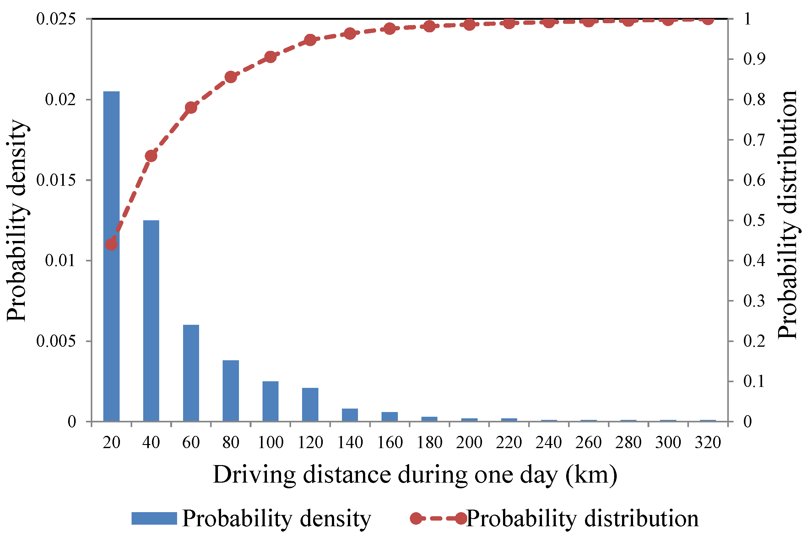
2.1. Modeling of the Power Demand and Supply of EVs

There are three mainstream interactive modes of EVs: normal interaction (NI), fast charging (FC), and battery exchange (BE). FC mode is detrimental to the battery, and introduces harmonic pollution to power systems. Therefore, this mode is not likely to be widely applied in the future, and our ED model only considers NI mode and BE mode.

The behavior characteristics of EV owners are determined by different uncertain factors (such as travel habit, vehicle type, and interactive mode), so their charging demand tends to be uncertain and difficult to be estimated with precision. Therefore, simplification is essential. In this paper, we use the following conditions and assumptions.

The analyses around EVs are derived from a prototype of the Nissan Leaf [25], which has a 160-km cruising radius, and a battery capacity of 24 kWh.

• The energy an EV has consumed is in direct proportion to the distance it has traveled.
• The probability distributions of an EV’s arrival time and the distance the EV has traveled are derived from driving pattern data collected in the National Household Transportation Survey (NHTS) [26].
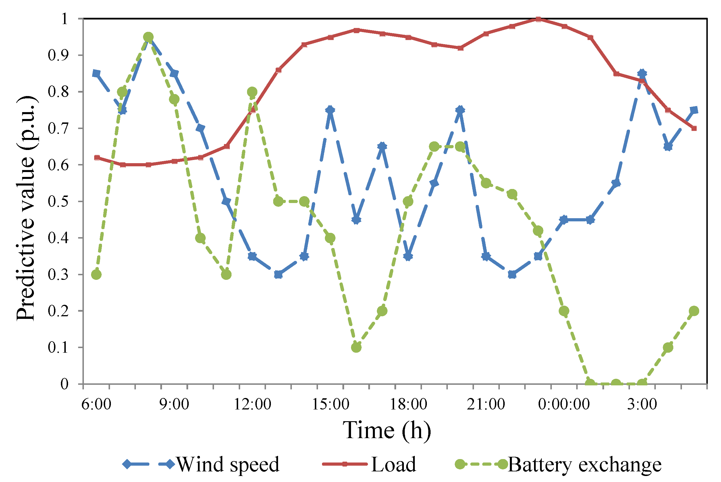
• The peaks of battery exchange demand are during the morning rush hour, lunch time, and afternoon rush hour.

We will now discuss the interactive modes of the EVs separately.

2.1.1. Power Demand and Supply of NI EVs

NI EVs are widely distributed in the daytime, making it difficult for them to follow scheduling instructions, so this model only considers night-time dispatch. Suppose some EV owners (proportion τ) sign the user agreement so that their car is connected to the power grid as soon as they finish the last trip in a day. In addition, suppose that they obey the dispatch plan so that the battery will be fully charged at 6:00 a.m. The NI EVs dispatch is a bi-level model: the upper dispatcher gives the plan to the NI stations, and the stations control the charging (or discharging), of the EVs. The stations communicate the condition of the EV to the upper dispatcher, such as unsatisfied demand of battery charging. The dispatch time is between 20:00 and 6:00 the next day, indicated as “NI schedulable period”.

To simplify our model, we assume that each EV charges/discharges in one specified NI station. For the EVs that sign the agreement with the NI station connected with bus k (indicated as “NI station k”), consider the penalty function at time t as:

(1)

(2)

where P_k,NI(t) is the interactive power between the system and the NI EVs signing the user agreement in bus k at time t. P_k,NI(t) is positive when the NI station is regarded as a load, negative when the NI station is regarded as a generator, and 0 if t is not a schedulable time. The penalty function is an approximate measure of the degree of non-satisfiability of the dispatch schedule. The first part represents the power dissatisfy, and the second part represents the energy dissatisfy.

The penalty of all NI stations is:

(3)

The EVs not signing the agreement are regarded as normal load. They start to charge as soon as finishing the last trip in a day, and continue until the battery is full. When connected to the power facilities, these EVs charge at power P_s.

2.1.2. Power Demand/Supply of BE EVs

In this mode, interaction between the EVs and the power system is implemented by battery exchange stations. At a given time t, the state of the BE station connected with bus m (indicated as “BE station m”) is described in Equation (4) [16], and the unmet demand of battery exchange can be calculated by Equation (5):

(4)

(5)

In Equations (4) and (5), P_m,BE(t) is positive when the BE station is regarded as a load and negative when the NI station is regarded as a generation. The penalty function for all BE stations is:

(6)

At a given time, the battery exchange demand is expected to follow a Poisson distribution:

(7)

We do not discuss the reactive demand and supply of EVs in this paper, as it is close to zero.

2.2. Modeling of Regular Load

We consider all other types of demand to be regular load and follow a random distribution. Therefore, a single probability distribution function can be used to describe this active/reactive demand at each bus. This distribution can be either derived from measurements or simply assumed to be the normal distribution N(μ_l,σ_l). We use the latter in this model.

2.3. Modeling of Wind Power

The output of a wind farm is considered to be in proportion to the third power of the wind speed:

(8)

where P_w(v) is the output of a wind farm when the wind speed is v. In Hetzer et al. [22] it was shown that wind speed follows a Weibull distribution:

(9)

The wind speed curve is given in Section 5. Assuming the power factor of a wind farm is constant, we can calculate the reactive power of wind farm using:

(10)

3. Economic Dispatch Formulation

3.1. Objective Function

By using an appropriate scheduling strategy, EVs can mitigate problems caused by the difference between power generation and demand at different times of the day, with minimized operational cost. We also need to meet the demand of EV charging. Thus, the objective function is:

(11)

The expressions of f_G, f_M, and f_P are as follows:

(12)

3.2. Constraints

We must minimize the objective function subject to a number of constraints.

• Power balance constraint:

P_W + P_G − P_{loss =} P_{EV +} P_L

(13)

• Generation limitation constraint:

(14)

• Power line transmission limitation constraint:

(15)

i → j indicates that bus i and bus j are connected by a power line.

• Local voltage limitation constraint:

(16)

• Normal interaction station operational constraint:

(17)

This constraint ensures that the dispatch schedule satisfies the EV owners’ requirements.

• Battery exchange station operational constraint:

(18)

(19)

Equation (19) ensures that the battery exchange station will operate sustainably. It is assumed that, to achieve a sustainable operation, the battery in BE stations should be full at the start and end of each day.

3.3. ED Problem Formulation

We can write the objective function in Equation (11) as:

C_total = f_obj(x,ξ)

(20)

where x represents the control variables (P_j,g(t), P_k,NI(t) and P_m,BE(t), j ≠ 1 because the conventional generator connected with Bus 1 is set as the balancing bus), and ξ represents the random variables (P_i,w(t), Q_k (t), and P_k,sev(t)). We can then formulate the economic dispatch problem as:

(21)

where g(x,ξ) is the equality constraint function and h(x,ξ) is the inequality constraint function.

4. Description of the Proposed Approach

We can conclude from Section 3 that this ED problem can be described as a high-dimensional, nonlinear, and stochastic model. Two classes of methods have been used in intelligent optimization algorithms to obtain the deterministic solution of a stochastic problem. The first is to establish an evaluation system of a solution in the stochastic environment, so that the stochastic problem can be transformed into a definite problem. Examples of this type of method include expectation derivation, stochastic simulation, and chance constrained programming (CCP) [27,28,29]. The other methods generate the current environment at each iteration using the mathematical description of the stochastic variables. One example is the continuous action-set learning automata (CALA) method [16]. This study proposes a FALA-based approach to address the ED problem.

4.1. The FALA Method

Learning automata (LA) are adaptive decision makers that learn to choose the optimal action from a set of available actions by using noisy reinforcement feedback from their environment [30]. LA can be divided into CALA and FALA according to whether the action is continuous or discrete. Only FALA is discussed in detail in this section.

Some definitions are given as follows: x is defined as a set of possible actions, f_obj(x,ξ) is defined as the response to the set of actions x obtained from the stochastic environment, the function F is defined as a reward function for the automation, which also is defined as the expectation of f_obj:

F(x) = E[f_obj(x,ξ)]

(22)

The goal of FALA is to find x where F(x) is (locally) minimized. It is difficult to calculate F analytically, as the underlying probability distribution that governs the reinforcement, f_obj, is unknown. In FALA, the feasible region is divided into limited areas. Suppose the amount of areas is r. In the beginning, the decision variable should obey a discrete probability distribution in the feasible region. During the iterative process, the algorithm updates this discrete probability distribution according to the response of the environment, until the probability that the decision variable lies in an area is close to 1. Each area can be represented by one variable (usually the intermediate points of the area, denoted by aⁱ for area i, i = 1, …, r). The discrete probability distribution can be represented by a vector, P(t) (the “action probability vector”), defined as:

P(t) = [p₁(t),…p_r(t)]

(23)

where p_i(t)(i = 1, ...,r) is the probability that the automaton will select the action aⁱ at time t, defined:

p_i(t) = p_r[x(t) = xⁱ],i = 1, ...,r

(24)

p_i(t) satisfies:

(25)

The FALA algorithm T: [0,1]^r × A × B → [0,1]^r is an updating scheme where A = {x₁, x₂, … x_r}, is the set of output actions of the automaton, and B is the response of the environment. Thus, the update is:

P(t + 1) = T(P(t), x(t),β(t))

(26)

where x(t) is the current value of the control variables at t^th iteration, generated based on the action probability vector P(t). β(t) is the response of the environment to x(t). β(t) is generally expressed as:

β(t) = B(f_obj(x(t),ξ(t)),flag,best(t))

(27)

where ξ(t) is the current value of the generated random variables, flag indicates if the constraints are satisfied, and best(t) is the historical minimum of the objective function.

4.2. FALA-Based Approach for the ED Problem

Our FALA approach is described as follows.

Step 1: The variables are initialized. The decision variable has n-dimensions (x = (x₁, …, x_n)) and each dimension is divided into M intervals, so the feasible region is divided into Mⁿ areas (r = Mⁿ). The action probability vector can be expressed by an n × M matrix, P_n,M(t), at the t^th iteration, where:

(28)

and p_i,j(t) represents the probability that x_i is selected for the j^th interval at time t. As mentioned, when selected from an interval, x_i willed be assigned as the midpoint of the interval.

Calculate the initial optimal value in the following way: all the stochastic variables are set to their expected value, and the interactive power between EV facilities is equal to the expected power demand of EVs. Then, calculate the output of the conventional generators using the optimal power flow method. The optimal value (best) is initialized to be the objective function (indicated as C_total(0)), i.e.:

best(0) = C_total(0)

(29)

Step 2: A set of random variables ξ(t) is generated using their respective probability distributions. The current values of P_i,w(t), Q_k(t), and P_k,sev(t) establish the current environment of the ED problem.

Step 3: A set of control actions x(t) is selected randomly based on the matrix P_n,M(t).

Step 4: The constraints are checked and the value of the objective function, f_obj(x(t),ξ(t)), is calculated. The variable flag is a symbol of whether the constraints are satisfied, defined as:

(30)

Step 5: Calculate the response of the environment using:

(31)

The response of the environment is 0 when the current control variables are “better” (constraints are satisfied and the total cost is small), the response is 1 when the current control variables are “worse”.

Step 6: Update the probability distributions of the actions. For the intervals that x_i (i = 1, …, n) are selected from, the probabilities are updated using:

(32)

For the other intervals, the probabilities are updated using:

(33)

In Equations (34) and (35), c is a constant representing the step size. These updates are derived from an intuitive idea: when the current control variables are “better” we increase the possibility that control variables are set as current values, otherwise the current control variables are “worse” and we increase the possibility that other values are used for the control variables.

Step 7: Update the current optimal value of objective function:

(34)

Step 8: Decide if the algorithm should terminate using:

(35)

where b is constant. If the inequality in Equation (35) is satisfied, the probability of the variable lying in an area is greater than bⁱ and the algorithm stops. If it is not satisfied, Steps 2–7 are repeated until the maximum number of iterations is reached. The flow chart of the FALA-based approach is shown in Figure 1.

Figure 1. Flow chart of the FALA-based approach.

Figure 1. Flow chart of the FALA-based approach.

5. Case Studies

A test system was developed based on the standard IEEE-30 bus system [31]. Bus 2 was connected with battery exchange stations, which had a total daily capacity of 2000 EVs. Bus 8 was connected with battery exchange stations, which has a total daily capacity of 1200 EVs. Buses 7, 21 were connected with 2000 EVs respectively using the NI mode, and the proportion of owners, τ, signing the user agreement was 50%. Two wind farms (with rated power of 10 MW) were connected to bus 2 and bus 13.

As previously mentioned, the number of cars arriving at the NI stations at each time interval and the driving distance of a day has been estimated using the driving pattern data collected in the NHTS [26]. The data are shown in Figure 2 and Figure 3.

Our examples assume that the energy consumed by an EV is proportional to the distance it has driven. The predictive probability of the battery exchange demand curve, conventional load demand curve, and predicative wind speed curve are shown in Figure 4. The rated wind speed is 14 m/s.

Other parameters used for these examples are: T = 1 h, C_w = 500 Ұ/MWh, C_NI = 1250 Ұ/MWh, C_BE = 1000 Ұ/MWh, C_un1 = C_un2 = C_un3 = 3000 Ұ/MWh, v_ci = 3 m/s, v_co = 22 m/s, P_R= 10 MW, P²_emin = −10 MW, P²_emax = 10 MW, P⁸_emin = −5 MW, P⁸_emax = 5 MW, E_max = 24 MWh, Uⁱ_min = 0.95, and Uⁱ_max = 1.05. The parameters of the conventional generators are listed in Table 1, and include the parameters of fuel cost and lower and upper limits of generation.

Figure 2. Driving pattern data: trip length [26].

Figure 2. Driving pattern data: trip length [26].

Figure 3. Driving pattern data: driving distance [26].

Figure 3. Driving pattern data: driving distance [26].

Figure 4. Power demand and wind farm output prediction.

Figure 4. Power demand and wind farm output prediction.

Table 1. Parameters of conventional generators.

Bus Number	α i (Ұ)	β i (Ұ/MW)	γi (Ұ/MW2)	(MW)	(MW)
1	0.124	12.4	0	0	80
2	0.1085	10.85	0	0	80
22	0.3875	6.2	0	0	50
27	0.5171	20.15	0	0	55
23	0.155	18.6	0	0	30
13	0.155	18.6	0	0	40

Table 1. Parameters of conventional generators.

Bus Number	α i (Ұ)	β i (Ұ/MW)	γi (Ұ/MW2)	(MW)	(MW)
1	0.124	12.4	0	0	80
2	0.1085	10.85	0	0	80
22	0.3875	6.2	0	0	50
27	0.5171	20.15	0	0	55
23	0.155	18.6	0	0	30
13	0.155	18.6	0	0	40

5.1. Parameter Settings

The parameters of FALA were set as: M = 10, r = 10²⁴, c = 0.02 and d = 0.01. The CALA-based approach is described in Yu et al. [16]. The parameters were set to: a = 0.001, b = 1000, and σ₀ = 0.01. The PSO-based (particle swarm optimization) approach is summarized as follows:

Step 1.

The stochastic problem was transformed into a deterministic problem using CCP (see [32] for details). The parameters were set as: N = 10, N’ = 8.

Step 2.

The transformed problem was solved using the PSO algorithm (see Equation (6) in [33]). The parameters were set as: Popsize = 20, φ_ic = 0.5, and φ₁ = φ₂ =2.

5.2. Results and Analysis

All programs were written using MATPOWER 4.1 [34] in MATLAB 2010b, and have been run on a desktop PC with an Inter^® Core™ i7-2600 3.40 GHz CPU, and 16 GB kst 4g/1333 RAM.

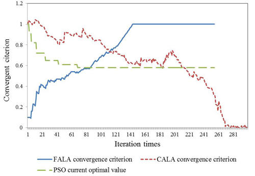
5.2.1. Comparison of Convergences

The convergence characteristics of the three algorithms are shown in Figure 5.

(1)

The convergence criterion of the FALA algorithm is given in Equation (35). It converged after approximately 150 iterations. In the first 30 iterations, the action probability vector changed rapidly because “best(t)” was not so small that the inequality constraint in Equation (36) was easily satisfied. During iterations 40–110 the action probability vector changed slowly as “best(t)” became smaller. After 120 iterations, the action probability vector had changed dramatically and there was a high probability that the control variables were selected in the optimal intervals, so the inequality in Equation (36) was easily satisfied. These results show that this algorithm is steady, and that, once converged, the action probability vector does not fluctuate:

best(t) > f_obj(x(t),ξ(t))

(36)

(2)

The CALA algorithm converged after approximately 270 iterations for this ED problem. The convergence criterion of the CALA algorithm fluctuated more dramatically than that of FALA algorithm, because it had the possibility to increase (opposite to the converging direction) even though the response of the current solution was good enough.

(3)

The characteristic curve of the PSO algorithm shows the change of the current global optimal value with each iteration. The value was transformed using:

best(t)′ = exp(100 × (best(t) − best(1))/best(1))

(37)

where best(t) is the global optimal value after t iterations. After approximately 70 iterations, the global optimal value no longer changed. Although the number of iterations was less than the LA algorithms, it did need more computing time because each iteration was much more complex. We will analyze this in the next section.

Figure 5. Convergence characteristics of three algorithms.

Figure 5. Convergence characteristics of three algorithms.

5.2.2. Comparison of Computation Efficiency

The main computation work needed for these algorithms was the power flow calculation. To calculate the objective function of one set of control variables in a deterministic environment, the computer needs to calculate the power flow 24 times. During each iteration, the FALA algorithm needs one objective function calculation; the CALA needs two, while the PSO needs 200 (the Popsize is 20, calculating the response of the environment of one pop using the CCP model requires N (=10) calculations of the objective function). The complexity and computing time of each algorithm is shown in Table 2.

Table 2. Algorithm complexity and computing time.

Algorithm	f0bj Calculation Times Each Iteration	Iteration Times	Total Times of f0bj Calculation	Computing Time(s)
FALA	1	160	160	239
CALA	2	270	540	815
PSO	200	70	14,000	15,872

Table 2. Algorithm complexity and computing time.

Algorithm	f0bj Calculation Times Each Iteration	Iteration Times	Total Times of f0bj Calculation	Computing Time(s)
FALA	1	160	160	239
CALA	2	270	540	815
PSO	200	70	14,000	15,872

5.2.3. Comparison of the Solution Quality

The environment is stochastic and the goal of the LA algorithms is to optimize the expectation of the environment’s response. Moreover, the LA algorithms do not establish an evaluation system of a solution in the stochastic environment. To compare the results of the three algorithms, each solution was tested in the stochastic environment 30 times (Table 3).

Table 3. Performance of algorithm results.

Algorithm	Mean Cost (Ұ)	Mean Diff (MW)	Mean Diff When Charging/Discharging Disorderly (MW)
FALA	57,939	62.53	92.02
CALA	57,925	60.48	91.62
PSO	57,970	63.91	94.80

Table 3. Performance of algorithm results.

Algorithm	Mean Cost (Ұ)	Mean Diff (MW)	Mean Diff When Charging/Discharging Disorderly (MW)
FALA	57,939	62.53	92.02
CALA	57,925	60.48	91.62
PSO	57,970	63.91	94.80

The results in Table 3 show that the mean cost of the results of the PSO algorithm is a little higher than that of the LA algorithms. This is because the goal of PSO is not to find the optimal solution in terms of the expected cost. The CCP model itself has established an evaluation system of a solution in the stochastic environment. If the correlation parameter was set properly in CCP, the PSO algorithm could also achieve an equivalent result to the LA algorithms.

We define Diff as the peak-value difference of thermal power-generating units. The algorithms can decrease the peak value by about 30%. The comprehensive load (including conventional load and EV load) when EVs and battery exchange stations charge/discharge orderly and disorderly are shown in Figure 6.

As seen in Figure 6, the scheduling of the EV station’s charging/discharging behavior can decrease the fluctuation of the comprehensive load demand, which is supplied by conventional generators and wind farms. Considering the dislocation between renewable resources and power demand that we mentioned in Section 1, the dispatch of EV stations can accommodate fluctuations in wind power in power systems.

Figure 6. Change of comprehensive load.

Figure 6. Change of comprehensive load.

6. Conclusions

In this paper, we have developed a stochastic ED model that considers a high penetration of EVs. Both the NI and BE modes are assumed to be schedulable in our model. We have proposed a FALA-based approach to solve the ED problem and compared the result with other two intelligent algorithms. Our results show that the FALA algorithm required less time than the CALA algorithm to reach the optimal solution, while PSO needed much more time than both. FALA can only converge to an interval, the measure of which is determined by the initial values. We conclude that the decrease in computation time of the FALA algorithm is obtained by sacrificing the accuracy. However, the results show that the accuracy of the FALA algorithm is satisfactory in the stochastic environment that we established in this paper. We also conclude that orderly charging of EVs can mitigate the fluctuation of load, and decrease the peak-value difference of thermal power-generating units.

However, the ED model developed in this paper should be used with caution. Considering the computation speed, the lower model of the NI station is not optimized, and the penalty functions (Equation (1) and Equation (5)) are only an approximation of the non-satisfiability of the dispatch schedule. The models in this paper should be further developed and more efficient stochastic optimization algorithms should be investigated before the techniques are applied.

References

1. Juul, N.; Meibom, P. Road transport and power system scenarios for Northern Europe in 2030. Appl. Energy 2012, 92, 573–582. [Google Scholar] [CrossRef]
2. Duvall, M.; Knipping, E.; Alexander, M. Environmental Assessment of Plug-in Hybrid Electric Vehicles; Volume 1, Nationwide Greenhouse Gas Emissions; Electric Power Research Institute: Palo Alto, CA, USA, 2007. [Google Scholar]
3. Liu, W.; Lund, H.; Mathiesen, B.V. Large-scale integration of wind power into the existing Chinese energy system. Energy 2011, 36, 4753–4760. [Google Scholar] [CrossRef]
4. Mathiesen, B.V.; Lund, H.; Karlsson, K. 100% Renewable energy systems, climate mitigation and economic growth. Appl. Energy 2011, 88, 488–501. [Google Scholar] [CrossRef]
5. Li, J.F.; Shi, P.F.; Gao, H. Wind Power Development Report in China; Hainan Press: Haikou, China, 2010. [Google Scholar]
6. Fernandez, L.P.; San Roman, T.G.; Cossent, R.; Domingo, C.M.; Frias, P. Assessment of the impact of plug-in electric vehicles on distribution networks. Power Syst. IEEE Trans. 2011, 26, 206–213. [Google Scholar] [CrossRef]
7. Clement-Nyns, K.; Haesen, E.; Driesen, J. The impact of charging plug-in hybrid electric vehicles on a residential distribution grid. Power Syst. IEEE Trans. 2010, 25, 371–380. [Google Scholar] [CrossRef] [Green Version]
8. Bessa, R.J.; Matos, M.A. Economic and technical management of an aggregation agent for electric vehicles: A literature survey. Electr. Power Eur. Trans. 2012, 22, 334–350. [Google Scholar] [CrossRef]
9. Rogers, K.M.; Klump, R.; Khurana, H.; Aquino-Lugo, A.A.; Overbye, T.J. An authenticated control framework for distributed voltage support on the smart grid. Smart Grid IEEE Trans. 2010, 1, 40–47. [Google Scholar] [CrossRef]
10. Lu, M.-S.; Chang, C.-L.; Lee, W.-J.; Wang, L. Combining the wind power generation system with energy storage equipment. Ind. Appl. IEEE Trans. 2009, 45, 2109–2115. [Google Scholar] [CrossRef]
11. Borba, B.; Szklo, A.; Schaeffer, R. Plug-in hybrid electric vehicles as a way to maximize the integration of variable renewable energy in power systems: The case of wind generation in northeastern Brazil. Energy 2012, 37, 469–481. [Google Scholar] [CrossRef]
12. Dallinger, D.; Gerda, S.; Wietschel, M. Integration of intermittent renewable power supply using grid-connected vehicles—A 2030 case study for California and Germany. Appl. Energy 2013, 104, 666–682. [Google Scholar] [CrossRef]
13. Markel, T.; Kuss, M.; Denholm, P. Communication and control of electric drive vehicles supporting renewables. In Proceedings of the IEEE Vehicle Power and Propulsion Conference, Dearborn, MI, USA, 7–10 September 2009; pp. 27–34.
14. Zhang, Y.; Gatsis, N.; Giannakis, G.B. Robust energy management for microgrids with high-penetration renewables. IEEE Trans. Sustain. Energy 2013, 4, 944–953. [Google Scholar]
15. Zhao, J.; Wen, F.; Dong, Z.Y.; Xue, Y.; Wong, K.-P. Optimal dispatch of electric vehicles and wind power using enhanced particle swarm optimization. IEEE Trans. Ind. Inf. 2012, 8, 889–899. [Google Scholar] [CrossRef]
16. Yu, H.J.; Gu, W.; Zhang, N.; Lin, D.Q. Economic dispatch considering integration of wind power generation and mixed-mode electric vehicles. In Proceedings of the IEEE Power and Energy Society General Meeting, San Diego, CA, USA, 22–26 July 2012; pp. 1–7.
17. Aghaei, J.; Ahmadi, A.; Shayanfar, H.A.; Rabiee, A. Mixed integer programming of generalized hydro-thermal self-scheduling of generating units. Electr. Eng. 2013, 95, 109–125. [Google Scholar] [CrossRef]
18. Silva, I.C.; do Nascimento, F.R.; de Oliveira, E.J.; Marcato, A.L.M.; de Oliveira, L.W.; Passos, J.A. Programming of thermoelectric generation systems based on a heuristic composition of ant colonies. Int. J. Electr. Power Energy Syst. 2013, 44, 134–145. [Google Scholar] [CrossRef]
19. Vo, D.N.; Ongsakul, W. Economic dispatch with multiple fuel types by enhanced augmented Lagrange Hopfield network. Appl. Energy 2012, 91, 281–289. [Google Scholar] [CrossRef]
20. Zhang, Y.; Gong, D.W.; Ding, Z.H. A bare-bones multi-objective particle swarm optimization algorithm for environmental/economic dispatch. Inf. Sci. 2012, 192, 213–227. [Google Scholar] [CrossRef]
21. Liu, X.; Xu, W. Economic load dispatch constrained by wind power availability: A here-and-now approach. IEEE Trans. Sustain. Energy 2010, 1, 2–9. [Google Scholar] [CrossRef]
22. Hetzer, J.; Yu, D.C.; Bhattarai, K. An economic dispatch model incorporating wind power. IEEE Trans. Energy Convers. 2008, 23, 603–611. [Google Scholar] [CrossRef]
23. Wu, L.; Shahidehpour, M.; Li, T. Stochastic security-constrained unit commitment. Power Syst. IEEE Trans. 2007, 22, 800–811. [Google Scholar] [CrossRef]
24. Gu, W.; Wu, Z.; Bo, R.; Liu, W.; Zhou, G.; Chen, W.; Wu, Z. Modeling, planning and optimal energy management of combined cooling, heating and power microgrid: A review. Int. J. Electr. Power Energy Syst. 2014, 54, 26–37. [Google Scholar] [CrossRef]
25. Hayes, J.G.; de Oliveira, R.P.R.; Vaughan, S.; Egan, M.G. Simplified electric vehicle power train models and range estimation. In Proceedings of the IEEE Vehicle Power and Propulsion Conference (VPPC), Chicago, IL, USA, 6–9 September 2011; pp. 1–5.
26. Santos, A.; McGuckin, N.; Nakamoto, H.Y.; Gray, D.; Liss, S. Summary of Travel Trends: 2009 National Household Travel Survey; Federal Highway Administration: Washington, DC, USA, 2009. [Google Scholar]
27. Gu, W.; Wu, Z.; Yuan, X. Microgrid economic optimal operation of the combined heat and power system with renewable energy. In proceedings of IEEE Power and Energy Society General Meeting, Minneapolis, MN, USA, 25–29 July 2010; pp. 1–6.
28. Wu, J.; Zhu, J.; Chen, G.; Zhang, H. A hybrid method for optimal scheduling of short-term electric power generation of cascaded hydroelectric plants based on particle swarm optimization and chance-constrained programming. Power Syst. IEEE Trans. 2008, 23, 1570–1579. [Google Scholar] [CrossRef]
29. Guan, Y.C.; Wang, Y.S.; Tan, Z.Y. Environmental protection and security considered dynamic economic dispatch for wind farm integrated systems. In Proceedings of the 2012 Asia-Pacific Power and Energy Engineering Conference, Shanghai, China, 27–29 May 2012; pp. 1–4.
30. Thathachar, M.; Sastry, P.S. Varieties of learning automata: An overview. IEEE Trans. Syst. Man Cybern. Part B Cybern. 2002, 32, 711–722. [Google Scholar] [CrossRef]
31. Kachore, P.; Palandurkar, M.V. TTC and CBM calculation of IEEE-30 bus system. In Proceedings of 2009 2nd International Conference on Emerging Trends in Engineering and Technology (ICETET), Nagpur, India, 16–18 December 2009; pp. 539–542.
32. Liu, B.D. Fuzzy random chance-constrained programming. Fuzzy Syst. IEEE Trans. 2001, 9, 713–720. [Google Scholar] [CrossRef]
33. Del Valle, Y.; Venayagamoorthy, G.K.; Mohagheghi, S.; Hernandez, J.C.; Harley, R.G. Particle swarm optimization: Basic concepts, variants and applications in power systems. IEEE Trans. Evol. Comput. 2008, 12, 171–195. [Google Scholar] [CrossRef]
34. Zimmerman, R.D.; Murillo-Sanchez, C.E.; Thomas, R.J. MATPOWER: Steady-state operations, planning, and analysis tools for power systems research and education. IEEE Trans. Power Syst. 2011, 26, 12–19. [Google Scholar] [CrossRef]