Circuit Simulation for Solar Power Maximum Power Point Tracking with Different Buck-Boost Converter Topologies ^†

Abstract

The power converter is one of the essential elements for effective use of renewable power sources. This paper focuses on the development of a circuit simulation model for maximum power point tracking (MPPT) evaluation of solar power that involves using different buck-boost power converter topologies; including SEPIC, Zeta, and four-switch type buck-boost DC/DC converters. The circuit simulation model mainly includes three subsystems: a PV model; a buck-boost converter-based MPPT system; and a fuzzy logic MPPT controller. Dynamic analyses of the current-fed buck-boost converter systems are conducted and results are presented in the paper. The maximum power point tracking function is achieved through appropriate control of the power switches of the power converter. A fuzzy logic controller is developed to perform the MPPT function for obtaining maximum power from the PV panel. The MATLAB-based Simulink piecewise linear electric circuit simulation tool is used to verify the complete circuit simulation model.

1. Introduction

Solar energy is the most abundant resource on Earth, and is expected to become one of the primary energy supply resources in the future [1,2]. Applications of solar energy are widespread in industrial, commercial, and military applications. However, effective use of solar energy depends on the technologies of solar power management systems. A power converter for maximal power point tracking (MPPT) and voltage or current regulation is inserted between the solar cell panel and the load to control power flow. This power converter directly affects the efficiency and performance of the solar power management system.

To maximize the use of available solar power drawn from the solar panel and to widen the applications of solar energy, several studies have investigated the design and applications of buck-boost converters [3,4,5,6,7]. Few studies have developed buck-boost converters for portable applications [4,5], whereas the study in [6] proposed a buck-boost-cascaded converter for high-power applications such as fuel-cell electric vehicles. Furthermore, an extensive analysis and design of Li-ion battery charging with the use of a four-switch type synchronous buck-boost power converter was presented in [7]. In the current research, we conducted a comparative study for MPPT evaluation by using different buck-boost converter topologies through circuit simulation, including Zeta, a single-ended primary-inductor converter (SEPIC), and four-switch type synchronous buck-boost converters.

The MPPT function is usually incorporated in solar power management systems to ensure that the maximum available power is received from the solar photovoltaic panel. Recently, the fuzzy logic controller has received increased attention from researchers for converter control and MPPT design [8,9,10,11,12,13,14]. Details and issues of the design of PV generators interfaced with MPP-tracking converters were reported in [15,16]. The results of [15,16] conclude that current-fed converters should be used for MPPT evaluation.

In the current study, we focused on circuit simulation for the buck-boost converter-based MPPT system. The primary purpose is to establish a circuit simulation environment so that the performance of the buck-boost converters and MPPT systems can be evaluated quickly without the need of any hardware systems and instruments. Dynamic analyses of the current-fed buck-boost converters (including SEPIC, Zeta, and four-switch type converters) were conducted. The results indicated that the small signal dynamics from control to input-voltage of the buck-boost converters are highly dependent on the operating region of the PV system and the duty ratio command for the converter. Following the dynamic analyses of the buck-boost converter systems, buck-boost converter-based MPPT systems were developed using the fuzzy logic to perform the MPPT function. Circuit simulations for the complete buck-boost converter-based MPPT system were successfully verified in the MATLAB/Simulink PLECS environment.

2. PV Model

Figure 1 presents the widely used single-diode equivalent circuit model to represent the characteristics of the PV panel for analyzing and simulating the PV system. The circuit model represents the PV panel as a current source $I_{ph}$ in parallel with a single diode and a shunt resistor $R_P$ as well as a series resistor $R_S$. The current $I_{PV}$ and voltage $V_{PV}$ from the PV panel is characterized by the following Equations (1) and (2):

$$I_{PV}=I_{ph}-I_D-\frac{V_{PV}+R_S{I}_{PV}}{R_P}$$

(1)

$$I_D=I_0\left[\exp \left(\frac{q(V_{PV}+R_S{I}_{PV})}{nAKT}\right)-1\right]$$

(2)

where $I_{ph}$ is the current generated by the incident light, $I_D$ is the diode current, $I_0$ is the reverse saturation current, $q$ is the electron charge (1.602 × 10−19 C), K is the Boltzmann constant (1.38 × 10−23 J/K), $T$ is the operating temperature of the cell in Kelvin (K), $A$ is the diode ideality constant, and $n$ is the number of diodes in series to form the single-diode model. The current source $I_{ph}$ mainly depends on the irradiation level of sun light as well as the operation temperature of the solar panel.

Figure 1. Single-diode equivalent circuit model.

Figure 1. Single-diode equivalent circuit model.

In this study, the Solarex MSX60 PV module was selected to conduct the design and circuit simulation. The key characteristics of the PV panel using previously published parameters [17] are listed in Table 1.

Table 1. Characteristics of the Solarex MSX 60 PV panel operate at 20 °C.

Parameter	Unit	Value
Irradiation Level, G	W/m2	1000
Temperature, T	°C	20
Open Circuit Voltage	V	21.5
Short Circuit Current	A	3.788
Voltage, Max Power	V	17.4
Current, Max Power	A	3.55
Maximum Power	W	61.77

Table 1. Characteristics of the Solarex MSX 60 PV panel operate at 20 °C.

Parameter	Unit	Value
Irradiation Level, G	W/m2	1000
Temperature, T	°C	20
Open Circuit Voltage	V	21.5
Short Circuit Current	A	3.788
Voltage, Max Power	V	17.4
Current, Max Power	A	3.55
Maximum Power	W	61.77

3. Buck-Boost Converter

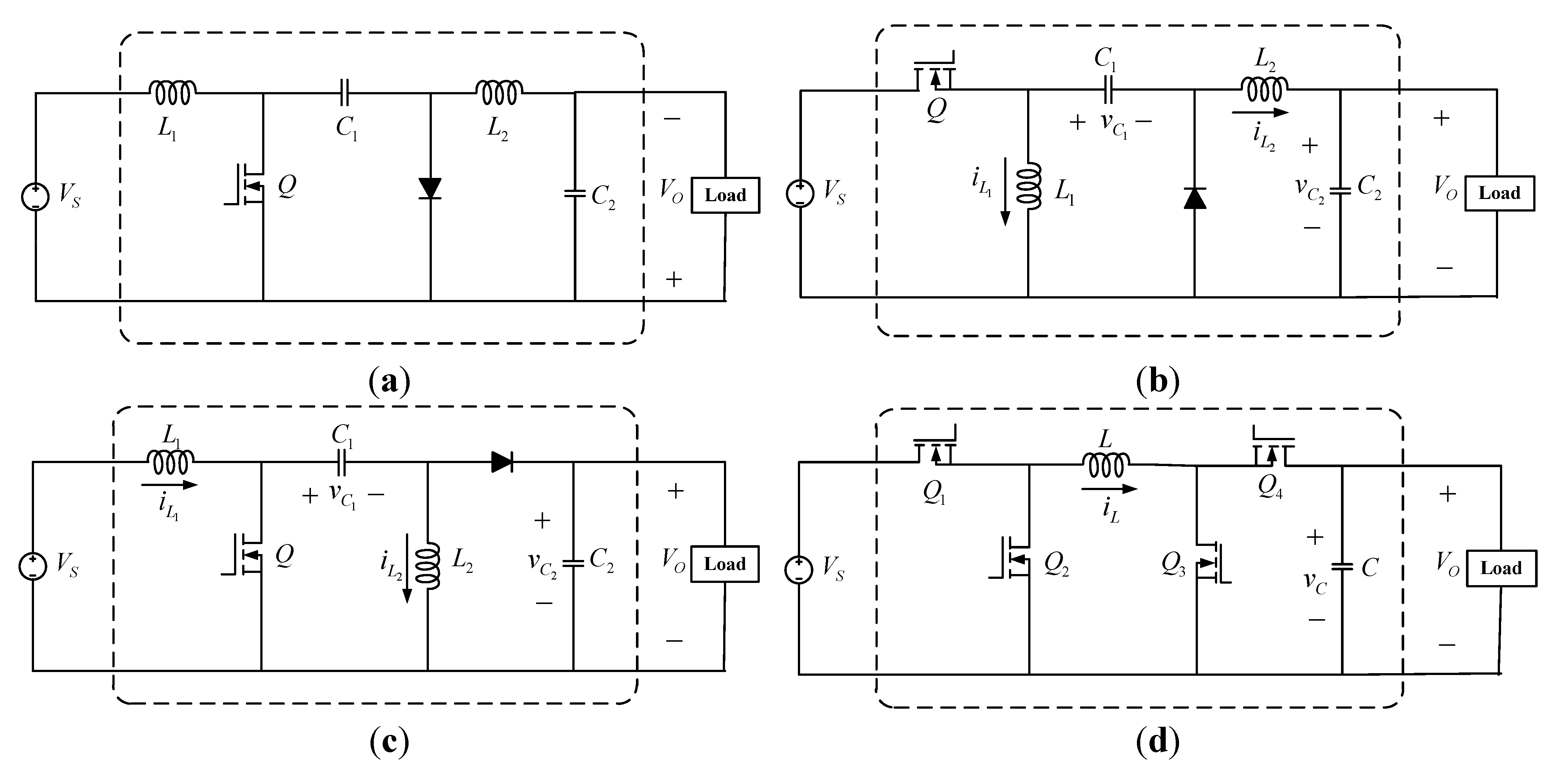
The buck-boost converter can convert the supply voltage source into higher and lower voltages at the load terminal. Several commonly used buck-boost converter topologies are shown in Figure 2. The Cuk converter in Figure 2a is an inverting type power converter (output voltage polarity is reversed), and the Zeta, SEPIC, and four-switch type topologies represented in Figure 2b–d are non-inverting buck-boost converters. The voltage at the load terminal is controlled by continuously adjusting the duty ratio of the power switch of the buck-boost converter. Because the voltage polarity at the load end is opposite to that at the source terminal of the Cuk converter, we examined only the non-inverting type buck-boost converter topologies (Figure 2b–d) in this study. Zeta and SEPIC converters contain two inductors, two capacitors, a diode, and a metal-oxide-semiconductor field-effect transistor (MOSFET) power switch. In addition, the four-switch type converter in Figure 2d is a synchronous buck-boost converter, containing an inductor, a capacitor, and four MOSFET power switches. The switches $Q_1$ and $Q_3$ work as one group, and $Q_2$ and $Q_4$ work as another group. When $Q_1$ and $Q_3$ are turned on, the switches $Q_2$ and $Q_4$ are turned off, and vice versa. In a steady-state condition, the output voltage of the non-inverting type buck-boost converter is:

$$V_O=\frac{D}{1-D}{V}_S$$

(3)

Thus, we can regulate the output voltage to higher or lower voltages compared with the source voltage by appropriately controlling the operating duty ratio for the MOSFET power switches.

Figure 2. Buck-Boost Converters. (a) Cuk converter; (b) Zeta Converter; (c) SEPIC Converter; (d) Four-switch type converter.

Figure 2. Buck-Boost Converters. (a) Cuk converter; (b) Zeta Converter; (c) SEPIC Converter; (d) Four-switch type converter.

To investigate the performance of the buck-boost converters, dynamic analyses of the non-inverting type converters (Figure 2b–d) were conducted first. The purpose of MPPT is to obtain the maximum power from the solar system. To maximize the efficiency of the buck-boost converter, the system is designed such that the converter is operated in continuous conducting mode. Therefore, we will only discuss the dynamic model of the converters operated in continuous conducting mode. 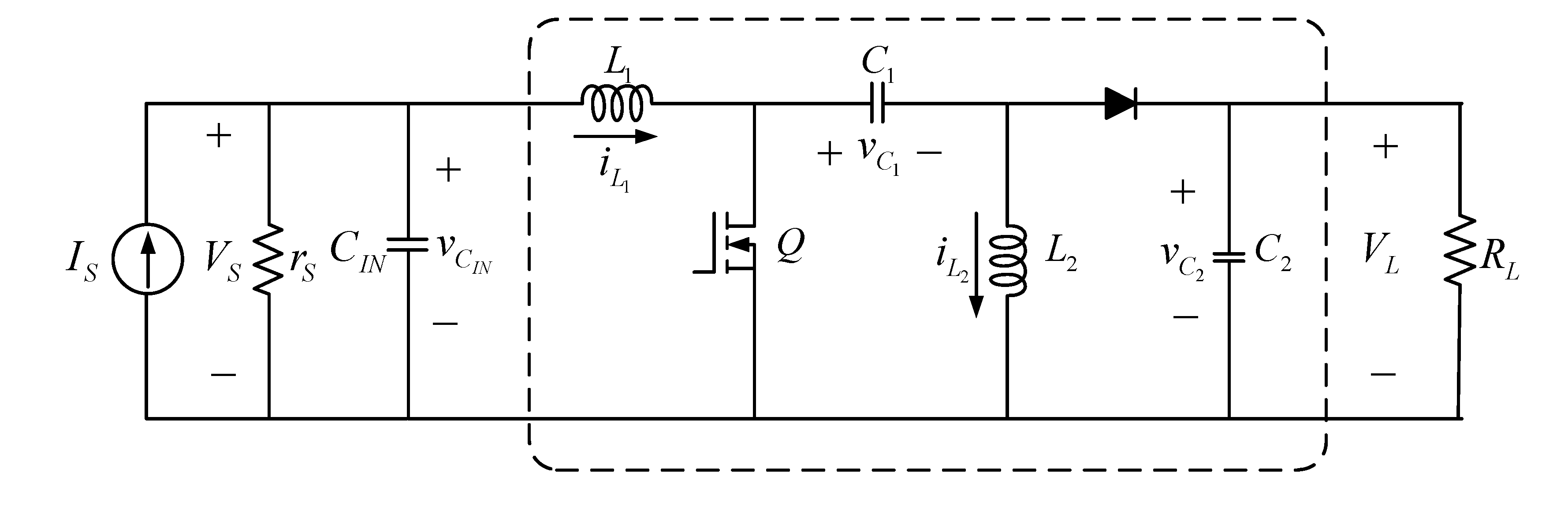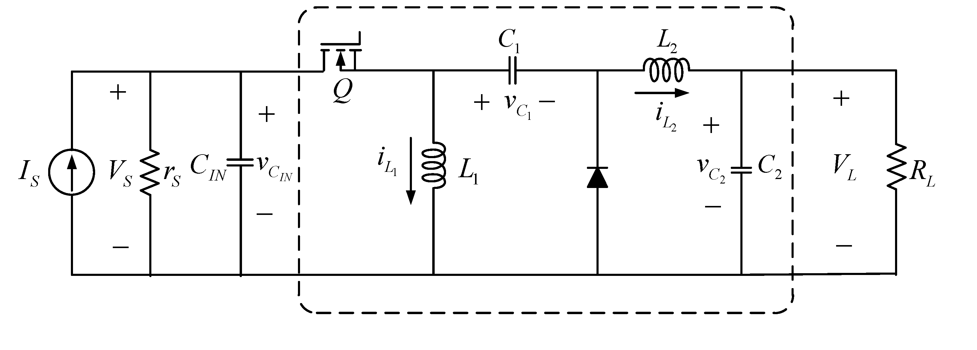According to [16], the converter is fed by a current source. The SEPIC buck-boost converter powered by a current source is shown in Figure 3. The input of the system is the source current $I_S$. The voltage at the input terminal, $V_S=v_{C_{IN}}$, is the output of the system for dynamic analysis. The resistor $r_S$ represents the internal resistance of the power source. An input capacitor $C_{IN}$ is included in this study. For simplicity, a resistive load is considered in this study. Using the variables defined in Figure 3 and taking the current flowing through the inductor $i_L$ and the voltage across the capacitor $v_C$ as the state of the converter, the averaged state-space model of the dynamics of the SEPIC converter is:

$$\begin{array}{c}\left[\begin{array}{c}\frac{d{v}_{C_{IN}}}{dt}\\ \frac{d{i}_{L_1}}{dt}\\ \frac{d{i}_{L_2}}{dt}\\ \frac{d{v}_{C_1}}{dt}\\ \frac{d{v}_{C_2}}{dt}\end{array}\right]=\left[\begin{array}{ccccc}-\frac{1}{r_S{C}_{IN}}& -\frac{1}{C_{IN}}& 0& 0& 0\\ \frac{1}{L_1}& 0& 0& -\frac{\left(1-D\right)}{L_1}& -\frac{\left(1-D\right)}{L_1}\\ 0& 0& 0& \frac{D}{L_2}& -\frac{\left(1-D\right)}{L_2}\\ 0& \frac{\left(1-D\right)}{C_1}& -\frac{D}{C_1}& 0& 0\\ 0& \frac{\left(1-D\right)}{C_2}& \frac{\left(1-D\right)}{C_2}& 0& \frac{-1}{C_2{R}_L}\end{array}\right]\left[\begin{array}{c}{v}_{C_{IN}}\\ i_{L_1}\\ i_{L_2}\\ v_{C_1}\\ v_{C_2}\end{array}\right]+\left[\begin{array}{c}\frac{1}{C_{IN}}\\ 0\\ 0\\ 0\\ 0\end{array}\right]I_S\\ \\ V_S=v_{C_{IN}}\end{array}$$

(4)

Figure 3. The current-fed SEPIC buck-boost converter circuit.

Figure 3. The current-fed SEPIC buck-boost converter circuit.

For investigating the performance of the buck-boost converter, dynamic analyses for duty-cycle variations were conducted. A small signal model was obtained by applying a small disturbance to the system and ignoring second order terms. If the duty cycle with a small disturbance is $D=\overline{D}+\tilde{d}$, the corresponding state and system output variations are $i_L={\overline{i}}_L+{\tilde{i}}_L$, $v_C={\overline{v}}_C+{\tilde{v}}_C$, and $V_S={\overline{V}}_S+{\tilde{v}}_{\text{S}}$. Variables $\overline{\phi }$ and $\tilde{\phi }$ represent the mean (or steady state) and variation of signal $\phi$. The small signal dynamic model driven by the small disturbance of duty cycle $\tilde{d}$, (the transfer function from control $\tilde{d}$ to the input-voltage ${\tilde{v}}_S$), is:

$$\begin{array}{c}\left[\begin{array}{c}\frac{d{\tilde{v}}_{C_{IN}}}{dt}\\ \frac{d{\tilde{i}}_{L_1}}{dt}\\ \frac{d{\tilde{i}}_{L_2}}{dt}\\ \frac{d{\tilde{v}}_{C_1}}{dt}\\ \frac{d{\tilde{v}}_{C_2}}{dt}\end{array}\right]=\left[\begin{array}{ccccc}-\frac{1}{r_S{C}_{IN}}& -\frac{1}{C_{IN}}& 0& 0& 0\\ \frac{1}{L_1}& 0& 0& -\frac{\left(1-\overline{D}\right)}{L_1}& -\frac{\left(1-\overline{D}\right)}{L_1}\\ 0& 0& 0& \frac{\overline{D}}{L_2}& -\frac{\left(1-\overline{D}\right)}{L_2}\\ 0& \frac{\left(1-\overline{D}\right)}{C_1}& -\frac{\overline{D}}{C_1}& 0& 0\\ 0& \frac{\left(1-\overline{D}\right)}{C_2}& \frac{\left(1-\overline{D}\right)}{C_2}& 0& \frac{-1}{R_L{C}_2}\end{array}\right]\left[\begin{array}{c}{\tilde{v}}_{C_{IN}}\\ {\tilde{i}}_{L_1}\\ {\tilde{i}}_{L_2}\\ {\tilde{v}}_{C_1}\\ {\tilde{v}}_{C_2}\end{array}\right]+\left[\begin{array}{c}0\\ \frac{1}{L_1}{\overline{v}}_{C_1}+\frac{1}{L_1}{\overline{v}}_{C_2}\\ \frac{1}{L_2}{\overline{v}}_{C_1}+\frac{1}{L_2}{\overline{v}}_{C_2}\\ -\frac{1}{C_1}{\overline{i}}_{L_1}-\frac{1}{C_1}{\overline{i}}_{L_2}\\ -\frac{1}{C_2}{\overline{i}}_{L_1}-\frac{1}{C_2}{\overline{i}}_{L_2}\end{array}\right]\tilde{d}\\ \\ {\tilde{v}}_S={\tilde{v}}_{C_{IN}}\end{array}$$

(5)

Using the MATLAB symbolic tool, the transfer equation of the system (5) can be rewritten as:

$$T(s)=K\frac{s^3+b_2{s}^2+b_{1}s+b_0}{s^5+a_4{s}^4+a_3{s}^3+a_2{s}^2+a_{1}s+a_0}$$

(6)

The gain and coefficients of the transfer Equation (6) are listed below:

$K=-\frac{{\overline{v}}_{C_1}+{\overline{v}}_{C_2}}{L_1{C}_{IN}}$$b_2=\frac{\left(C_1+C_2\right)\left({\overline{i}}_{L_1}+{\overline{i}}_{L_2}\right)\left(1-\overline{D}\right)}{C_1{C}_2\left({\overline{v}}_{C_1}+{\overline{v}}_{C_2}\right)}+\frac{1}{R_L{C}_2}$

$b_1=\frac{\left({\overline{i}}_{L_1}+{\overline{i}}_{L_2}\right)\left(1-\overline{D}\right)}{C_1{C}_2{R}_L\left({\overline{v}}_{C_1}+{\overline{v}}_{C_2}\right)}+\frac{\overline{D}}{L_2{C}_1}$$b_0=\frac{\left({\overline{i}}_{L_1}+{\overline{i}}_{L_2}\right)\left(1-\overline{D}\right)}{C_1{C}_2{L}_2\left({\overline{v}}_{C_1}+{\overline{v}}_{C_2}\right)}+\frac{\overline{D}}{C_1{C}_2{L}_2{R}_L}$

$a_4=\frac{1}{r_S{C}_{IN}}+\frac{1}{R_L{C}_2}$$a_3=\frac{1}{L_1}\left[\frac{{\left(1-\overline{D}\right)}^2}{C_1}+\frac{{\left(1-\overline{D}\right)}^2}{C_2}+\frac{1}{C_{IN}}\right]+\frac{1}{L_2}\left[\frac{{\overline{D}}^2}{C_1}+\frac{{\left(1-\overline{D}\right)}^2}{C_2}\right]+\frac{1}{C_2{C}_{IN}{R}_L{r}_S}$

$a_2=\frac{L_2\left[C_1+C_{IN}{\left(1-\overline{D}\right)}^2\right]+L_1{C}_{IN}{\overline{D}}^2}{L_1{L}_2{C}_1{C}_2{C}_{IN}{R}_L}+\frac{\left[L_1{C}_1+L_2\left(C_1+C_2\right)\right]{\left(1-\overline{D}\right)}^2+L_1{C}_2{\overline{D}}^2}{L_1{L}_2{C}_1{C}_2{C}_{IN}{r}_S}$

$a_1=\frac{L_1{\overline{D}}^2+L_2{\left(1-\overline{D}\right)}^2}{L_1{L}_2{C}_1{C}_2{C}_{IN}{R}_L{r}_S}+\frac{\left(C_1+C_2\right){\left(1-\overline{D}\right)}^2+C_2{\overline{D}}^2}{L_1{L}_2{C}_1{C}_2{C}_{IN}}$$a_0=\frac{R_L{\left(1-\overline{D}\right)}^2+r_S{\overline{D}}^2}{L_1{L}_2{C}_1{C}_2{C}_{IN}{R}_L{r}_S}$

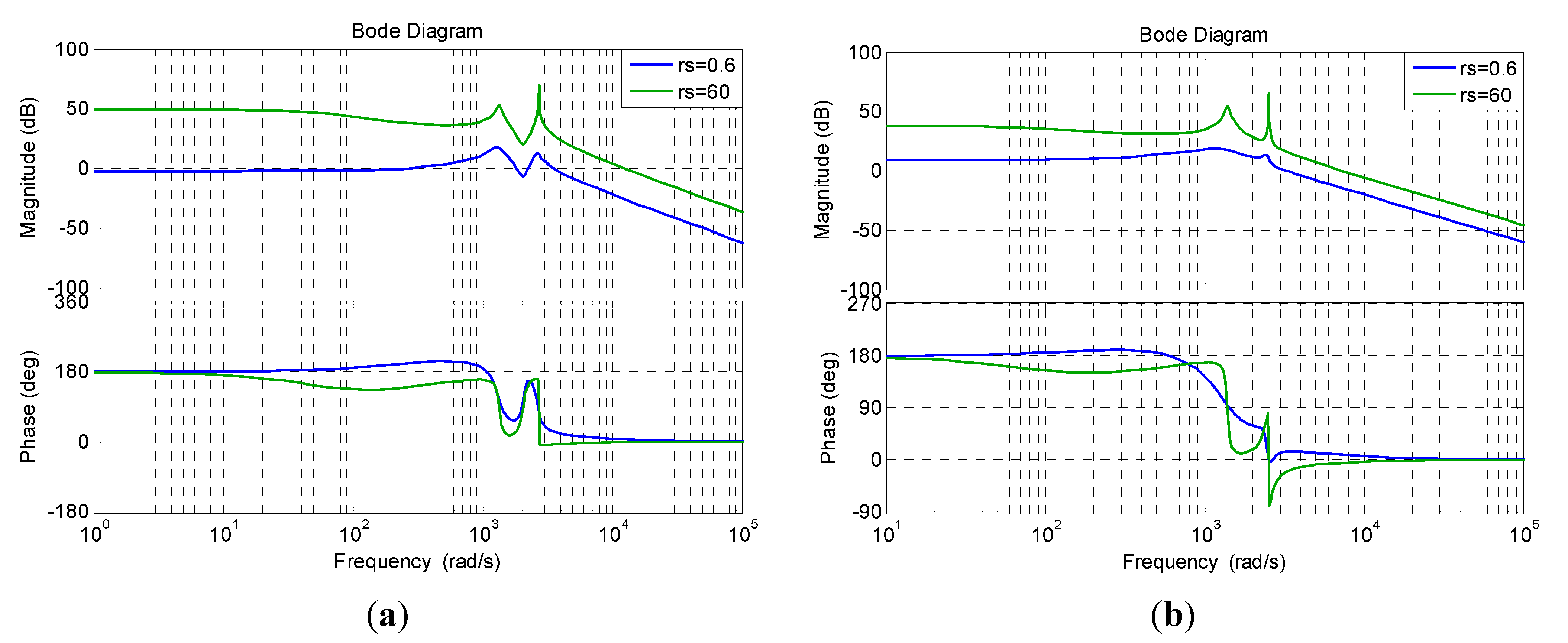
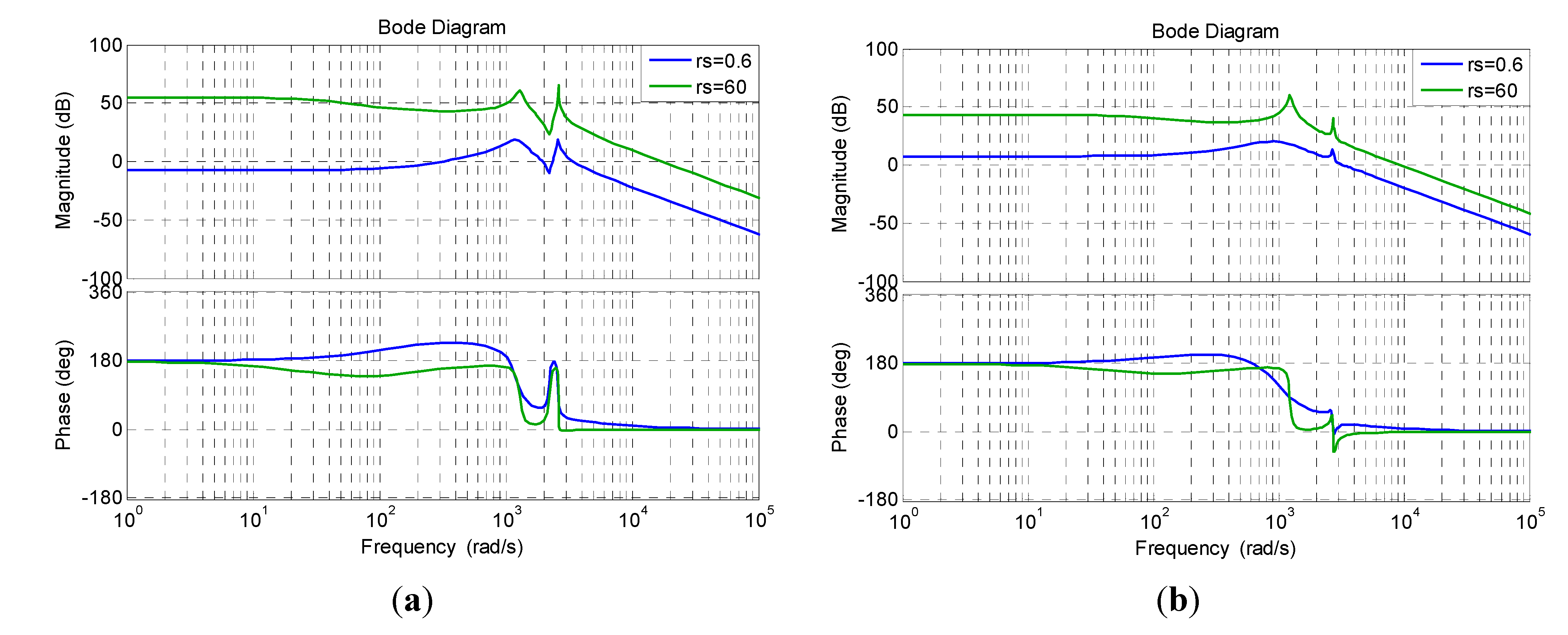
From Equation (6), the dynamic behavior of the converter depends on the duty ratio command ($\overline{D}$) and the source resistance ($r_S$). The duty ratio command affects the pole and zero locations of the small signal dynamics, while the source resistance only affects the pole locations of the system. If the converter is powered by solar modules, the resistance may represent the dynamic resistance of the solar system. The Bode plots of the small signal dynamics Equation (5) of the SEPIC converter with $L_1=L_2=470\mu \text{H}$, $C_{IN}=C_2=1000\mu \text{F}$, $C_1=200\mu \text{F}$, and $R_L=6\Omega$ are shown in Figure 4. Figure 4a contains the results of buck operations with different source resistance. The lower source resistance $r_S=0.6\Omega$) represents that the solar module is operated in the constant voltage region, while the higher source resistance ($r_S=60\Omega$) represents that the solar module is operated in the constant current region. The results for boost operations are shown in Figure 4b. The results indicate that the source resistance has a profound effect on the dynamic characteristic of the system.

.

Figure 4. Bode plots of the SEPIC converter. (a) $\overline{D}=0.4$; (b) $\overline{D}=0.6$.

Figure 4. Bode plots of the SEPIC converter. (a) $\overline{D}=0.4$; (b) $\overline{D}=0.6$.

Using the similar techniques, a state-space representation of the dynamics of the current-fed Zeta converter, as shown in Figure 5, operated in continuous conducting mode can be obtained as:

$$\begin{array}{c}\left[\begin{array}{c}\frac{d{v}_{C_{IN}}}{dt}\\ \frac{d{i}_{L_1}}{dt}\\ \frac{d{i}_{L_2}}{dt}\\ \frac{d{v}_{C_1}}{dt}\\ \frac{d{v}_{C_2}}{dt}\end{array}\right]=\left[\begin{array}{ccccc}-\frac{1}{r_S{C}_{IN}}& -\frac{1}{C_{IN}}& 0& 0& 0\\ \frac{d}{L_1}& 0& 0& -\frac{(1-D)}{L_1}& 0\\ 0& 0& 0& \frac{D}{L_2}& -\frac{1}{L_2}\\ 0& \frac{(1-D)}{C_1}& -\frac{D}{C_1}& 0& 0\\ 0& 0& \frac{1}{C_2}& 0& -\frac{1}{R_L{C}_2}\end{array}\right]\left[\begin{array}{c}{v}_{C_{IN}}\\ i_{L_1}\\ i_{L_2}\\ v_{C_1}\\ v_{C_2}\end{array}\right]+\left[\begin{array}{c}\frac{1}{C_{IN}}\\ 0\\ 0\\ 0\\ 0\end{array}\right]I_S\\ V_S=v_{C_{IN}}\end{array}$$

(7)

Figure 5. The current-fed Zeta buck-boost converter circuit.

Figure 5. The current-fed Zeta buck-boost converter circuit.

The small signal dynamic model driven by the small disturbance of duty cycle $\tilde{d}$ is:

$$\begin{array}{c}\left[\begin{array}{c}\frac{d{\tilde{v}}_{C_{IN}}}{dt}\\ \frac{d{\tilde{i}}_{L_1}}{dt}\\ \frac{d{\tilde{i}}_{L_2}}{dt}\\ \frac{d{\tilde{v}}_{C_1}}{dt}\\ \frac{d{\tilde{v}}_{C_2}}{dt}\end{array}\right]=\left[\begin{array}{ccccc}-\frac{1}{r_S{C}_{IN}}& -\frac{1}{C_{IN}}& 0& 0& 0\\ \frac{\overline{D}}{L_1}& 0& 0& -\frac{(1-\overline{D})}{L_1}& 0\\ 0& 0& 0& \frac{\overline{D}}{L_2}& -\frac{1}{L_2}\\ 0& \frac{(1-\overline{D})}{C_1}& -\frac{\overline{D}}{C_1}& 0& 0\\ 0& 0& \frac{1}{C_2}& 0& -\frac{1}{R_L{C}_2}\end{array}\right]\left[\begin{array}{c}{\tilde{v}}_{C_{IN}}\\ {\tilde{i}}_{L_1}\\ {\tilde{i}}_{L_2}\\ {\tilde{v}}_{C_1}\\ {\tilde{v}}_{C_2}\end{array}\right]+\left[\begin{array}{c}0\\ \frac{1}{L_1}{\overline{v}}_{C_{IN}}+\frac{1}{L_1}{\overline{v}}_{C_1}\\ \frac{1}{L_2}{\overline{v}}_{C_1}\\ -\frac{1}{C_1}{\overline{i}}_{L_1}-\frac{1}{C_1}{\overline{i}}_{L_2}\\ 0\end{array}\right]\tilde{d}\\ \\ {\tilde{V}}_S={\tilde{v}}_{C_{IN}}\end{array}$$

(8)

The dynamics of Equation (8) expressed in transfer function form is:

$$T(s)=K\frac{s^3+b_2{s}^2+b_{1}s+b_0}{s^5+a_4{s}^4+a_3{s}^3+a_2{s}^2+a_{1}s+a_0}$$

(9)

The gain and coefficients of the transfer Equation (9) are listed below:

$K=-\frac{{\overline{V}}_S+{\overline{v}}_{C_1}}{L_1{C}_{IN}}$$b_2=\frac{\left({\overline{i}}_{L_1}+{\overline{i}}_{L_2}\right)\left(1-\overline{D}\right)}{C_1\left({\overline{V}}_S+{\overline{v}}_{C_1}\right)}+\frac{1}{R_L{C}_2}$

$b_1=\frac{\left({\overline{i}}_{L_1}+{\overline{i}}_{L_2}\right)\left(1-\overline{D}\right)}{C_1{C}_2{R}_L\left({\overline{V}}_S+{\overline{v}}_{C_1}\right)}+\frac{1}{L_2{C}_2}+\frac{\left({\overline{v}}_{C_1}+{\overline{V}}_S\overline{D}\right)\overline{D}}{L_2{C}_1\left({\overline{V}}_S+{\overline{v}}_{C_1}\right)}$$b_0=\frac{\left({\overline{i}}_{L_1}+{\overline{i}}_{L_2}\right)\left(1-\overline{D}\right)}{C_1{C}_2{L}_2\left({\overline{V}}_S+{\overline{v}}_{C_1}\right)}+\frac{\left({\overline{v}}_{C_1}+{\overline{V}}_S\overline{D}\right)\overline{D}}{C_1{C}_2{L}_2{R}_L\left({\overline{V}}_S+{\overline{v}}_{C_1}\right)}$

$a_4=\frac{1}{r_S{C}_{IN}}+\frac{1}{R_L{C}_2}$$a_3=\frac{1}{L_1}\left[\frac{\overline{D}}{C_{IN}}+\frac{{\left(1-\overline{D}\right)}^2}{C_1}\right]+\frac{1}{L_2}\left(\frac{1}{C_2}+\frac{{\overline{D}}^2}{C_1}\right)+\frac{1}{C_2{C}_{IN}{R}_L{r}_S}$

$a_2=\frac{1}{r_S{C}_{IN}}\left[\frac{{\left(1-\overline{D}\right)}^2}{L_1{C}_1}+\frac{1}{L_2{C}_2}+\frac{{\overline{D}}^2}{L_2{C}_1}\right]+\frac{1}{R_L{C}_2}\left[\frac{{\left(1-\overline{D}\right)}^2}{L_1{C}_1}+\frac{{\overline{D}}^2}{L_2{C}_1}+\frac{\overline{D}}{L_1{C}_{IN}}\right]$

$a_1=\frac{L_1{\overline{D}}^2+L_2{\left(1-\overline{D}\right)}^2}{C_1{C}_2{C}_{IN}{L}_1{L}_2{R}_L{r}_S}+\frac{1}{L_1{L}_2}\left[\frac{{\left(1-\overline{D}\right)}^2}{C_1{C}_2}+\frac{\overline{D}}{C_2{C}_{IN}}+\frac{{\overline{D}}^3}{C_1{C}_{IN}}\right]$$a_0=\frac{r_S{\overline{D}}^3+R_L{\left(1-\overline{D}\right)}^2}{C_1{C}_2{C}_{IN}{L}_1{L}_2{R}_L{r}_S}$

From Equation (9), it is clear that the source resistance will not affect the zero locations of the dynamic system. The Bode plots using the same parameters for the SEPIC converter are shown in Figure 6. The results in Figure 6 also indicate that the dynamic behavior of the converter is highly dependent on the magnitude of the source resistance.

Figure 6. Bode plots of the Zeta converter. (a) $\overline{D}=0.4$; (b) $\overline{D}=0.6$.

Figure 6. Bode plots of the Zeta converter. (a) $\overline{D}=0.4$; (b) $\overline{D}=0.6$.

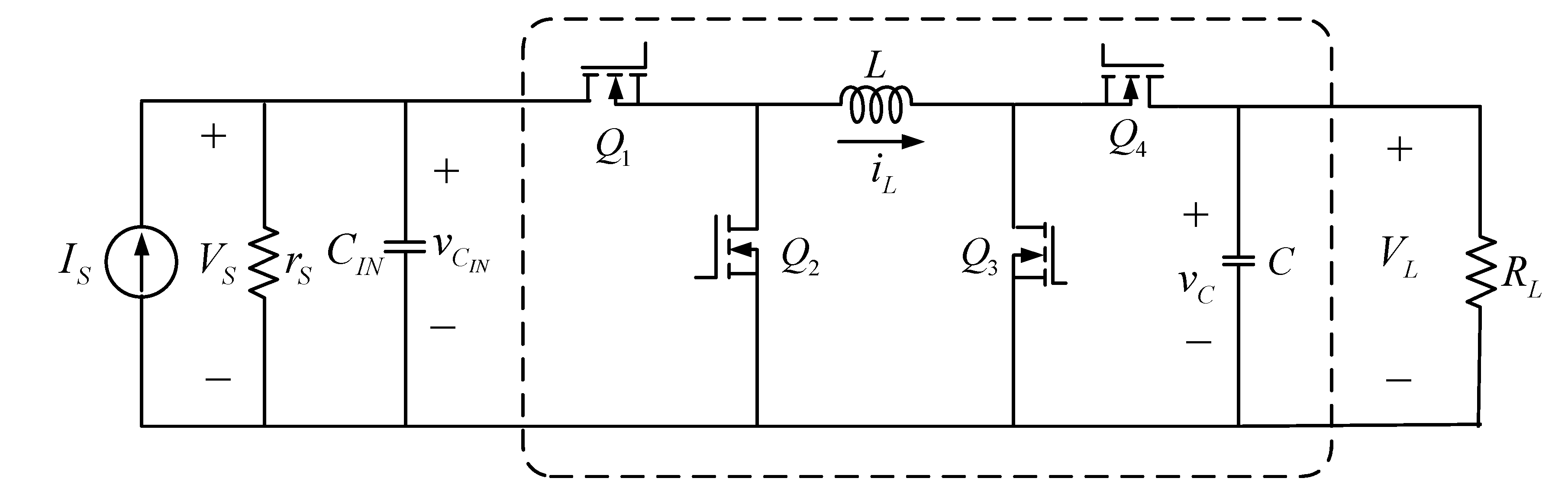
Similarly, a state-space form of the dynamics of the current-fed four-switch type converter, as shown in Figure 7, operated in continuous conducting mode is given by:

$$\begin{array}{c}\left[\begin{array}{c}\frac{d{v}_{C_{IN}}}{dt}\\ \frac{d{i}_L}{dt}\\ \frac{d{v}_C}{dt}\end{array}\right]=\left[\begin{array}{ccc}-\frac{1}{r_S{C}_{IN}}& -\frac{D}{C_{IN}}& 0\\ \frac{D}{L}& 0& -\frac{\left(1-D\right)}{L}\\ 0& \frac{\left(1-D\right)}{C}& -\frac{1}{R_{L}C}\end{array}\right]\left[\begin{array}{c}{v}_{C_{IN}}\\ i_L\\ v_C\end{array}\right]+\left[\begin{array}{c}\frac{D}{C_{IN}}\\ 0\\ 0\end{array}\right]I_S\\ \\ V_S=v_{C_{IN}}\end{array}$$

(10)

Figure 7. The current-fed four-switch type buck-boost converter circuit.

Figure 7. The current-fed four-switch type buck-boost converter circuit.

The small signal dynamic model from $\tilde{d}$ to ${\tilde{v}}_S$ is:

$$\begin{array}{c}\left[\begin{array}{c}\frac{d{\tilde{v}}_{C_{IN}}}{dt}\\ \frac{d{\tilde{i}}_L}{dt}\\ \frac{d{\tilde{v}}_C}{dt}\end{array}\right]=\left[\begin{array}{ccc}-\frac{1}{r_S{C}_{IN}}& -\frac{\overline{D}}{C_{IN}}& 0\\ \frac{\overline{D}}{L}& 0& -\frac{\left(1-\overline{D}\right)}{L}\\ 0& \frac{\left(1-\overline{D}\right)}{C}& -\frac{1}{R_{L}C}\end{array}\right]\left[\begin{array}{c}{\tilde{v}}_{C_{IN}}\\ {\tilde{i}}_L\\ {\tilde{v}}_C\end{array}\right]+\left[\begin{array}{c}-\frac{1}{C_{IN}}{\overline{i}}_L\\ \frac{1}{L}{\overline{v}}_{C_{IN}}+\frac{1}{L}{\overline{v}}_C\\ -\frac{1}{C}{\overline{i}}_L\end{array}\right]\tilde{d}\\ \\ {\tilde{v}}_S={\tilde{v}}_{C_{IN}}\end{array}$$

(11)

The dynamics of system Equation (11) expressed in transfer function form is:

$$T(s)=\frac{-\frac{{\overline{i}}_L}{C_{IN}}\left\{s^2+\left[\frac{1}{R_{L}C}+\frac{\left({\overline{V}}_S+{\overline{v}}_C\right)\overline{D}}{L{\overline{i}}_L}\right]s+\left[\frac{1-\overline{D}}{LC}+\frac{\left({\overline{V}}_S+{\overline{v}}_C\right)\overline{D}}{R_{L}LC{\overline{i}}_L}\right]\right\}}{s^3+\left[\frac{1}{r_S{C}_{IN}}+\frac{1}{R_{L}C}\right]s^2+\left[\frac{{\left(1-\overline{D}\right)}^2}{LC}+\frac{{\overline{D}}^2}{L{C}_{IN}}+\frac{1}{r_S{R}_{L}C{C}_{IN}}\right]s+\frac{1}{LC{C}_{IN}}\left[\frac{{\left(1-\overline{D}\right)}^2}{r_S}+\frac{{\overline{D}}^2}{R_L}\right]}$$

(12)

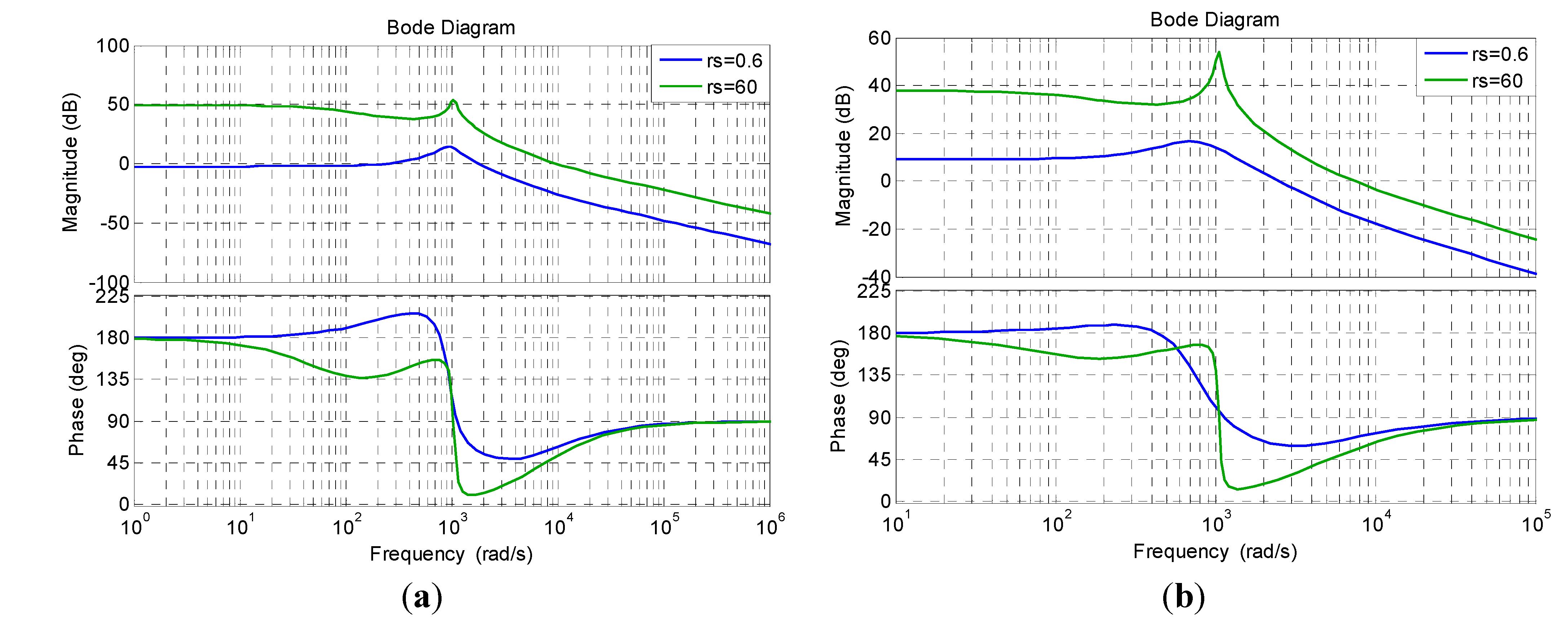
The Bode plots of the four-switch type converter are shown in Figure 8. Obviously, the results in Figure 8 also indicate that the dynamic behavior of the converter highly depends on the magnitude of the source resistance.

Figure 8. Bode plots of the Four-Switch type converter. (a) $\overline{D}=0.4$; (b) $\overline{D}=0.6$.

Figure 8. Bode plots of the Four-Switch type converter. (a) $\overline{D}=0.4$; (b) $\overline{D}=0.6$.

From the above discussion, the small signal dynamics from control to input-voltage of the buck-boost converters considered in this study are highly dependent on the internal resistance of the power source. That is, if the converter is powered by a solar system, the dynamic characteristics depend on the operating region of the solar system. All of the three buck-boost converters are used for the circuit simulation in this study. For simplicity and easy of demonstration, resistive loads are considered in the circuit simulations. The results are presented in the following sections.

It is worth noting that if the control dynamics to output-voltage of the converters are considered, both poles and zeros of the system depend on the source resistance and the duty ratio command. Moreover, the system contains right-half plane zeros. The number and locations of the right-half plane zeros also depend on the source resistance and the duty ratio command. The right-half plane zeros cause constraints on the design of control system. Control of the output-voltage of the converter is not in the scope of this paper. Therefore, we will not discuss the details of the dynamics of the system from control to output-voltage of the converter in this paper.

4. Buck-Boost Converter-Based MPPT System

The operating point of the PV panel varies when the load condition varies. The maximum power point may be achieved through appropriate load selection. In most cases, the load is not likely to be optimal (regarding maximum power delivered from the PV panel). Maximum power from the PV panel may be attained by incorporating an intelligent mechanism to alter the load resistance observed from the PV panel. Power converters are widely used to adjust operating conditions to attain the maximum power point.

Figure 9 depicts the incorporation of a buck-boost converter into a PV system. The input voltage is controlled through appropriate adjustments of the duty ratio of the power switches of the converter. Assuming that the buck-boost converter is operating in the continuous conducting mode with 100% efficiency, the relationship of the voltage and current at the load terminal and those at the PV panel under steady-state conditions are:

$$V_o=\frac{D}{1-D}{V}_{PV};I_o=\frac{1-D}{D}{I}_{PV}$$

(13)

Based on Ohm’s law, the load resistance can be expressed as:

$$R_L=\frac{V_o}{I_o}={\left(\frac{D}{1-D}\right)}^2\frac{V_{PV}}{I_{PV}}$$

(14)

Thus, the equivalent resistance observed from the PV panel, denoted as $R_{PV}$, is:

$$R_{PV}=\frac{V_{PV}}{I_{PV}}={\left(\frac{1-D}{D}\right)}^2{R}_L$$

(15)

Equation (15) implies that for a certain load resistance $R_L$, the equivalent resistance $R_{PV}$ depends only on the duty ratio of the buck-boost converter. Hence, we may adjust the duty ratio D to achieve maximum power transfer from the PV panel through an optimal mechanism. Figure 10 presents the power characteristics of the PV system and power received at the load terminal with different duty ratios for the power switches of the converter. The power developed at the load terminal is:

$$P_L=\frac{V_o^2}{R_L}=\frac{{\left(\frac{D}{1-D}{V}_{PV}\right)}^2}{R_L}={\left(\frac{D}{1-D}\right)}^2\frac{V_{PV}^2}{R_L}=\frac{V_{PV}^2}{R_{PV}}$$

(16)

The intersection of the PV power curve (blue) and the power curve for the load (red) was the operating point of the PV system. The maximum power point may be achieved by applying the appropriate duty ratio for the power converter. In this study, a fuzzy logic controller was designed to perform the MPPT function.

Figure 9. PV system with buck-boost converter incorporated.

Figure 9. PV system with buck-boost converter incorporated.

Figure 10. Power characteristics of the PV system.

Figure 10. Power characteristics of the PV system.

5. Fuzzy Logic MPPT Controller

The fuzzy logic control system is depicted in Figure 11, and the input variables of this controller are the slope of the power variation $E(n)$ and the change of the slope $\Delta E(n)$ defined as:

$$E(n)=\frac{P(n)-P(n-1)}{V_{PV}(n)-V_{PV}(n-1)}$$

(17)

$$\Delta E(n)=E(n)-E(n-1)$$

(18)

The output variable of the fuzzy logic controller is the increment $\Delta D$ of the duty-ratio command for the power switches. Based on the characteristics of the PV model and the features of the buck-boost converter (Figure 10), a five-term fuzzy set, Negative Big (NB), Negative Small (NS), Zero (ZE), Positive Small (PS), and Positive Big (PB), were defined to describe each linguistic variable. The fuzzy rules for this MPPT design are listed in Table 2. Figure 12 describes the membership functions for the input and output variables. The Mamdani fuzzy method was used in this buck-boost converter-based circuit simulation, in which the maximum of the minimum composition technique was used for the inference, and the center of gravity was used for the defuzzification process.

Figure 11. Fuzzy logic controller for the MPPT design.

Figure 11. Fuzzy logic controller for the MPPT design.

Table 2. Fuzzy rule table.

Fuzzy rules		E(n)
		NB	NS	ZE	PS	PB
∆E(n)	NB	ZE	PS	PS	ZE	NS
	NS	PB	PS	ZE	ZE	NS
	ZE	PB	PS	ZE	NS	NB
	PS	PS	ZE	ZE	NS	NB
	PB	PS	ZE	NS	NS	ZE

Table 2. Fuzzy rule table.

Fuzzy rules		E(n)
		NB	NS	ZE	PS	PB
∆E(n)	NB	ZE	PS	PS	ZE	NS
	NS	PB	PS	ZE	ZE	NS
	ZE	PB	PS	ZE	NS	NB
	PS	PS	ZE	ZE	NS	NB
	PB	PS	ZE	NS	NS	ZE

Figure 12. Membership functions for the input and output variables.

Figure 12. Membership functions for the input and output variables.

The circuit simulation model for the buck-boost converter based MPPT system and its PLECS circuit are illustrated in Figure 13. Three resistive loads (3 Ω, 4.9 Ω, and 8 Ω) were used to evaluate the performance of the fuzzy controller.

Figure 13. Circuit simulation model for buck-boost converter based MPPT system with its PLECS circuit.

Figure 13. Circuit simulation model for buck-boost converter based MPPT system with its PLECS circuit.

6. Results and Discussion

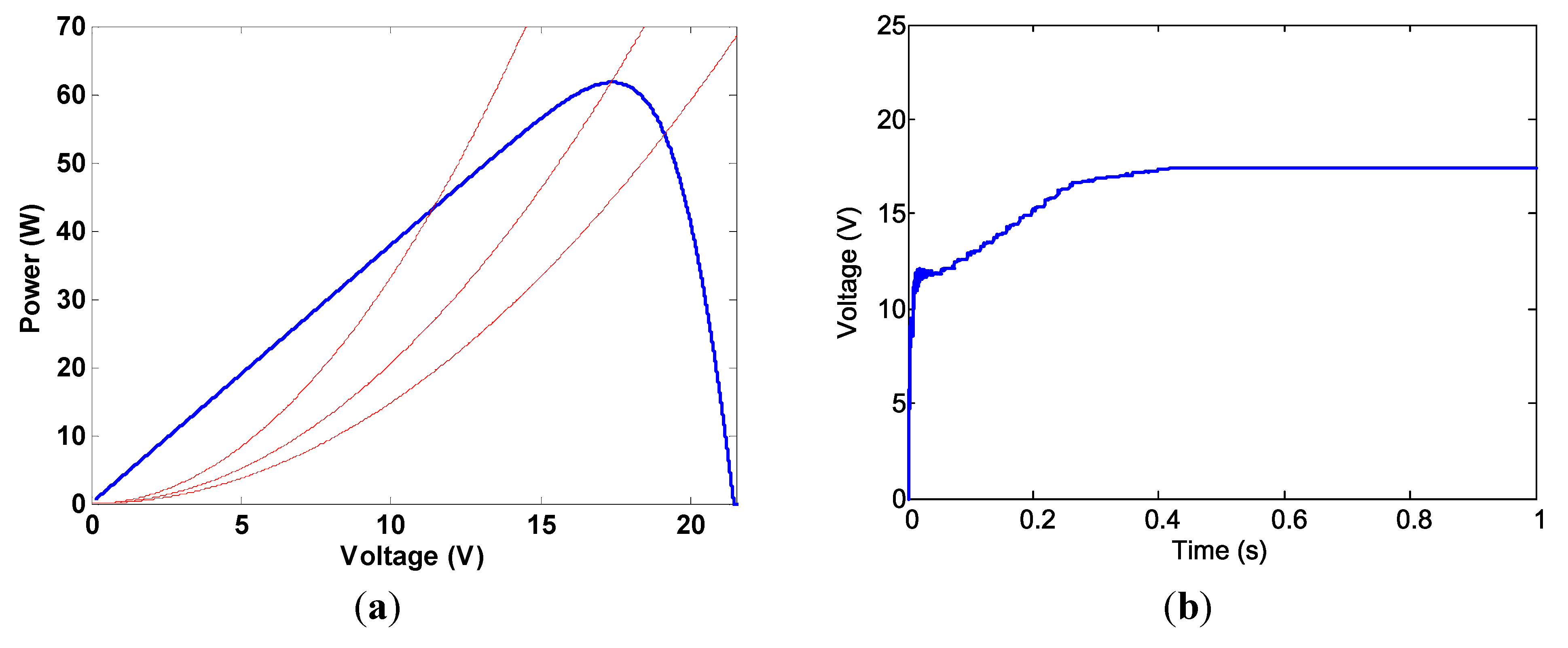
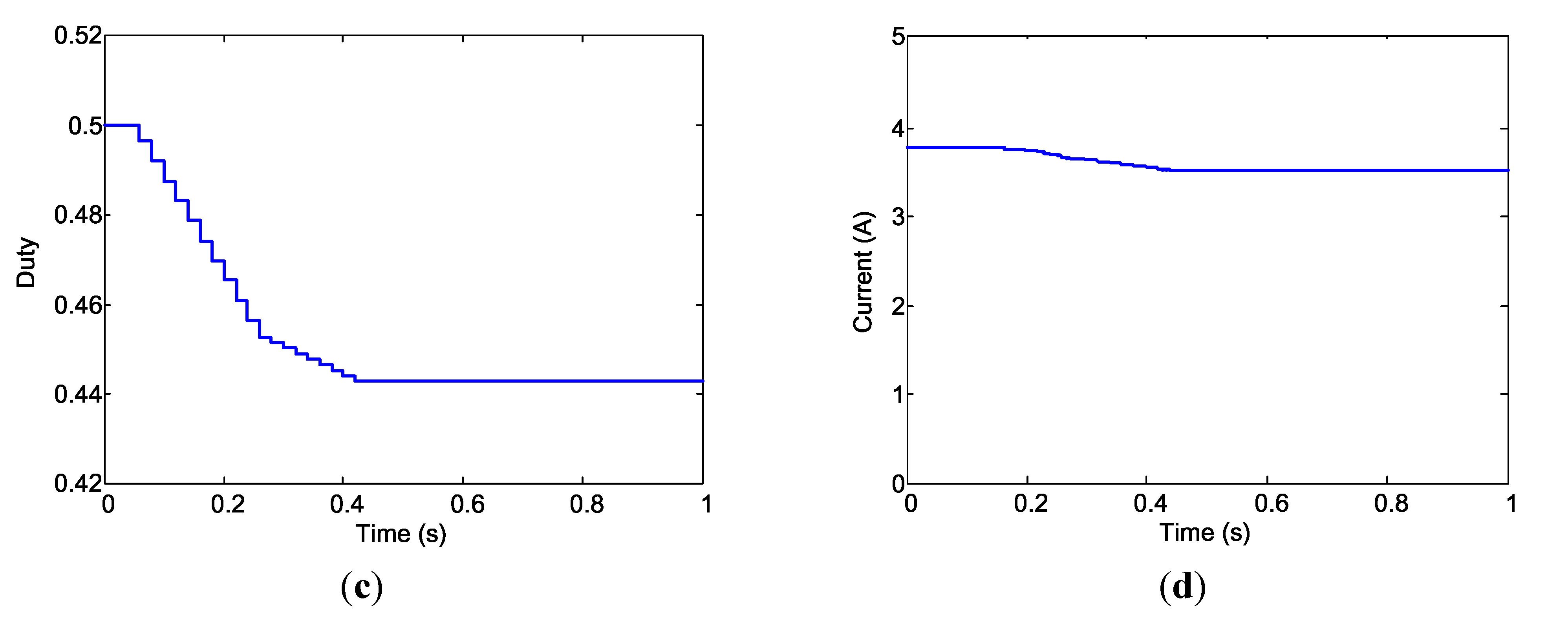
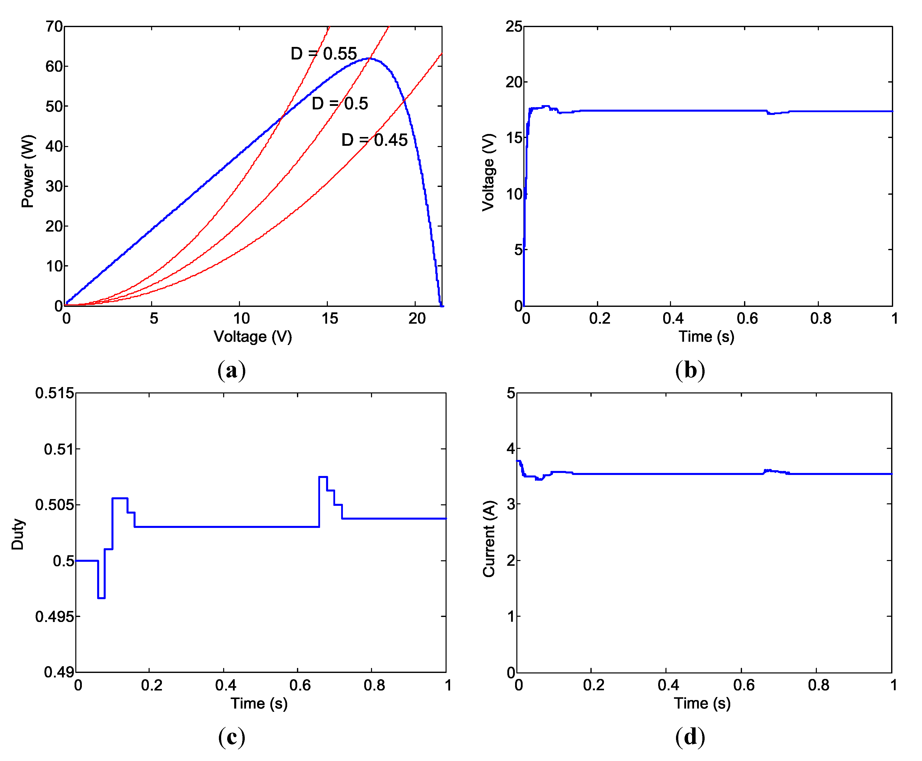
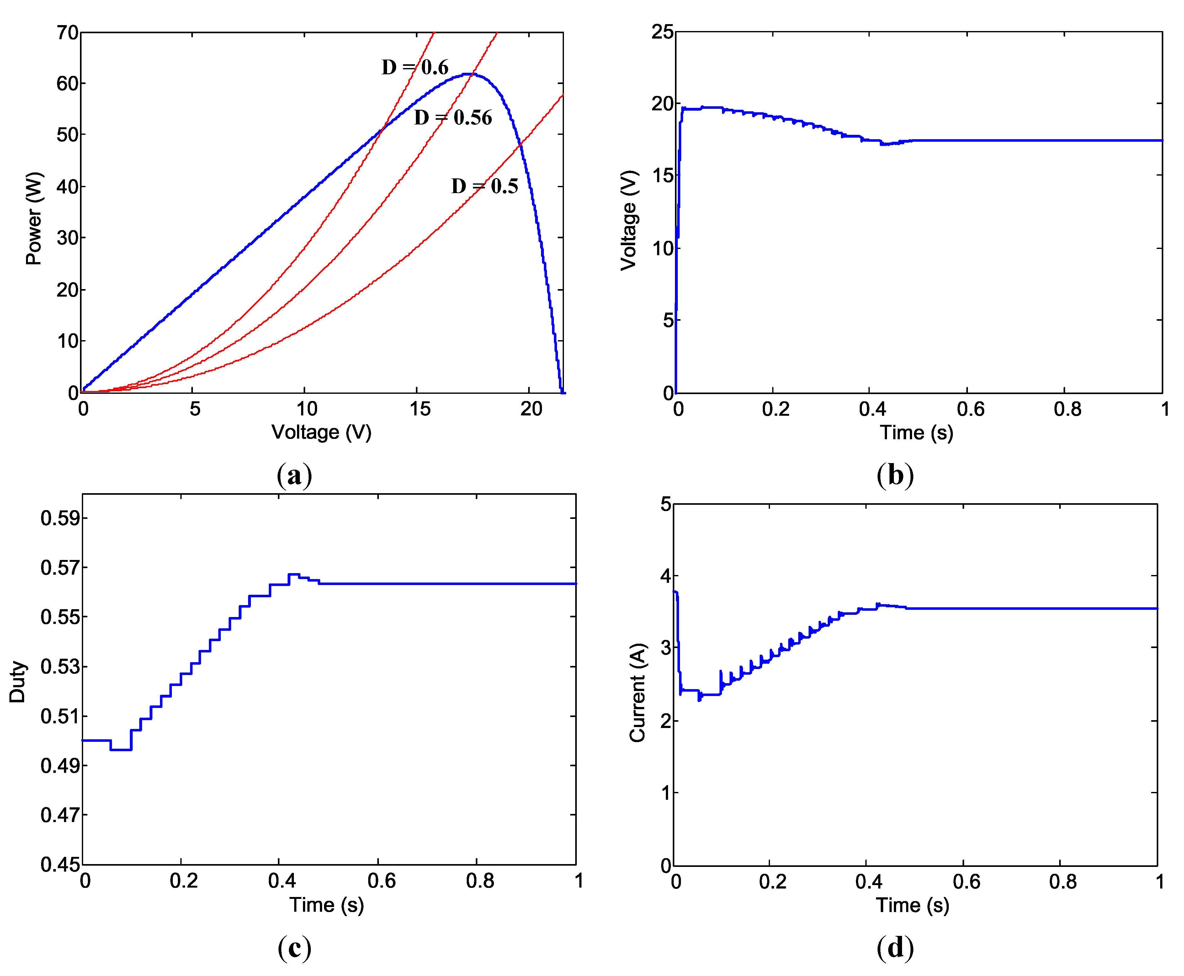
The voltage and current outputs from the PV model for the SEPIC buck-boost converter MPPT system loaded with different resistive loads are presented in Figure 14, Figure 15 and Figure 16. Figure 14 shows the results for the 3 Ω resistive load. Figure 14a represents the power characteristics of the PV panel and power curve for different duty ratios. The analytical value of the duty ratio for the maximum power point is 0.44 for the 3 Ω load resistor. The voltage and current from the PV model are 17.44 V and 3.54 A, respectively. The steady-state duty ratio from the fuzzy controller is 0.4428 (Figure 14b). The results perfectly matched the maximum power point, as expected.

Figure 14. Figure 14. Circuit simulation results with 3 Ω load. (a) Power characteristics; (b) Duty ratio command; (c) Output voltage from PV model; (d) Output current from PV model.

Figure 14. Figure 14. Circuit simulation results with 3 Ω load. (a) Power characteristics; (b) Duty ratio command; (c) Output voltage from PV model; (d) Output current from PV model.

The results for 4.9 Ω and 8 Ω loads are shown in Figure 15 and Figure 16. As mentioned, the maximum power points were obtained. Similar results were achieved for Zeta and four-switch type buck-boost converters. The results of the MPPT circuit simulations are summarized in Table 3. The maximum power points were almost perfectly reached for any combination of the power converters and loads discussed in this study.

Figure 15. Figure 15. Circuit simulation results with 4.9 Ω load. (a) Power characteristics; (b) Duty ratio command; (c) Output voltage from PV model; (d) Output current from PV model.

Figure 15. Figure 15. Circuit simulation results with 4.9 Ω load. (a) Power characteristics; (b) Duty ratio command; (c) Output voltage from PV model; (d) Output current from PV model.

Figure 16. Circuit simulation results with 8 Ω load. (a) Power characteristics; (b) Duty ratio command; (c) Output voltage from PV model; (d) Output current from PV model.

Figure 16. Circuit simulation results with 8 Ω load. (a) Power characteristics; (b) Duty ratio command; (c) Output voltage from PV model; (d) Output current from PV model.

Table 3. Summaries of the MPPT circuit simulations results.

Converter	Zeta			SEPIC			Four-Switch
Load	3 Ω	4.9 Ω	8 Ω	3 Ω	4.9 Ω	8 Ω	3 Ω	4.9 Ω	8 Ω
VPV (V)	17.473	17.419	17.378	17.448	17.377	17.418	17.33	17.425	17.363
IPV (A)	3.5425	3.5462	3.5529	3.54	3.5548	3.5464	3.5632	3.545	3.5577
PPV (W)	61.77	61.772	61.773	61.768	61.772	61.771	61.75	61.772	61.772
Duty Ratio	0.4428	0.5031	0.5638	0.4428	0.5038	0.5635	0.4473	0.5050	0.5667

Table 3. Summaries of the MPPT circuit simulations results.

Converter	Zeta			SEPIC			Four-Switch
Load	3 Ω	4.9 Ω	8 Ω	3 Ω	4.9 Ω	8 Ω	3 Ω	4.9 Ω	8 Ω
VPV (V)	17.473	17.419	17.378	17.448	17.377	17.418	17.33	17.425	17.363
IPV (A)	3.5425	3.5462	3.5529	3.54	3.5548	3.5464	3.5632	3.545	3.5577
PPV (W)	61.77	61.772	61.773	61.768	61.772	61.771	61.75	61.772	61.772
Duty Ratio	0.4428	0.5031	0.5638	0.4428	0.5038	0.5635	0.4473	0.5050	0.5667

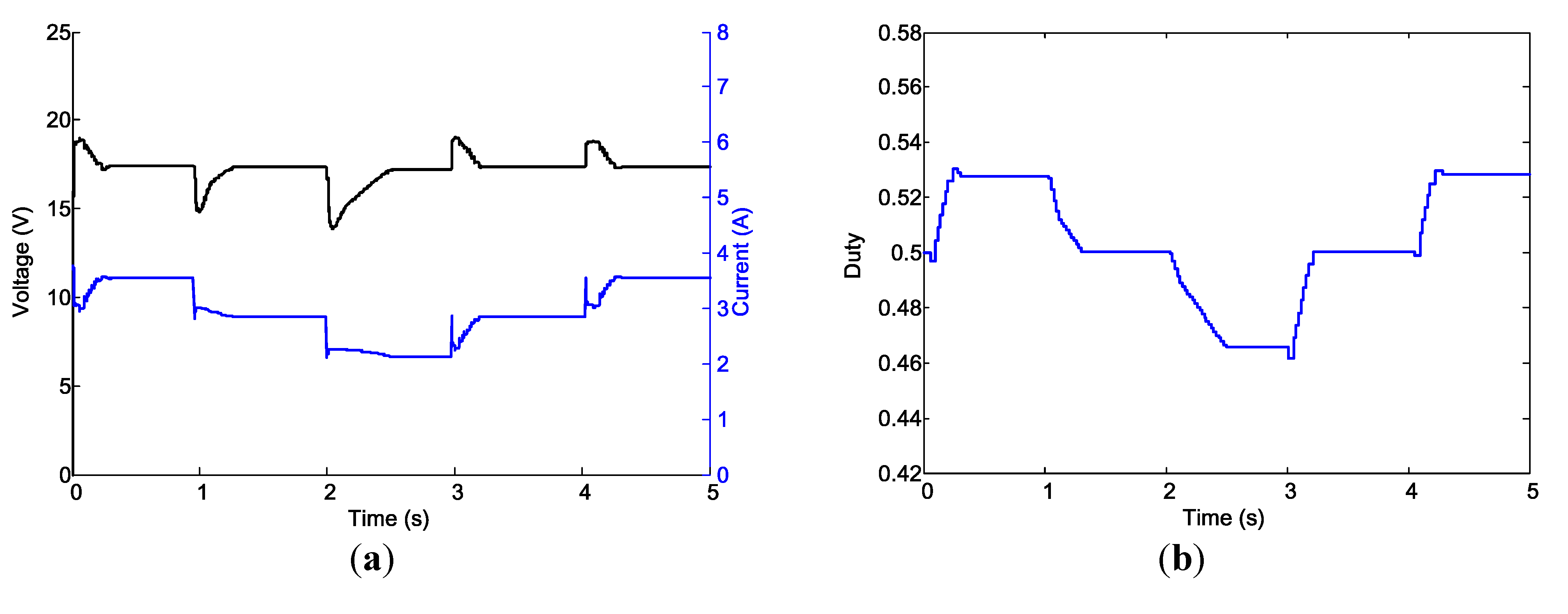
The results shown in Table 3 demonstrate the success of the MPPT simulation for different load conditions. Another important feature of the MPPT function is that it can adapt to variations in irradiance. Circuit simulations for variations of the irradiation levels were also conducted in this study. The sequence of the irradiation level was $G=1.0\to G=0.8\to G=0.6\to G=0.8\to G=1.0$ in this simulation. A 6 Ω load was used for this simulation to ensure that buck and boost operations were covered in the simulation. The duration for each irradiation level was one second. The results for using SEPIC for MPPT function are shown in Figure 17 and Figure 18. 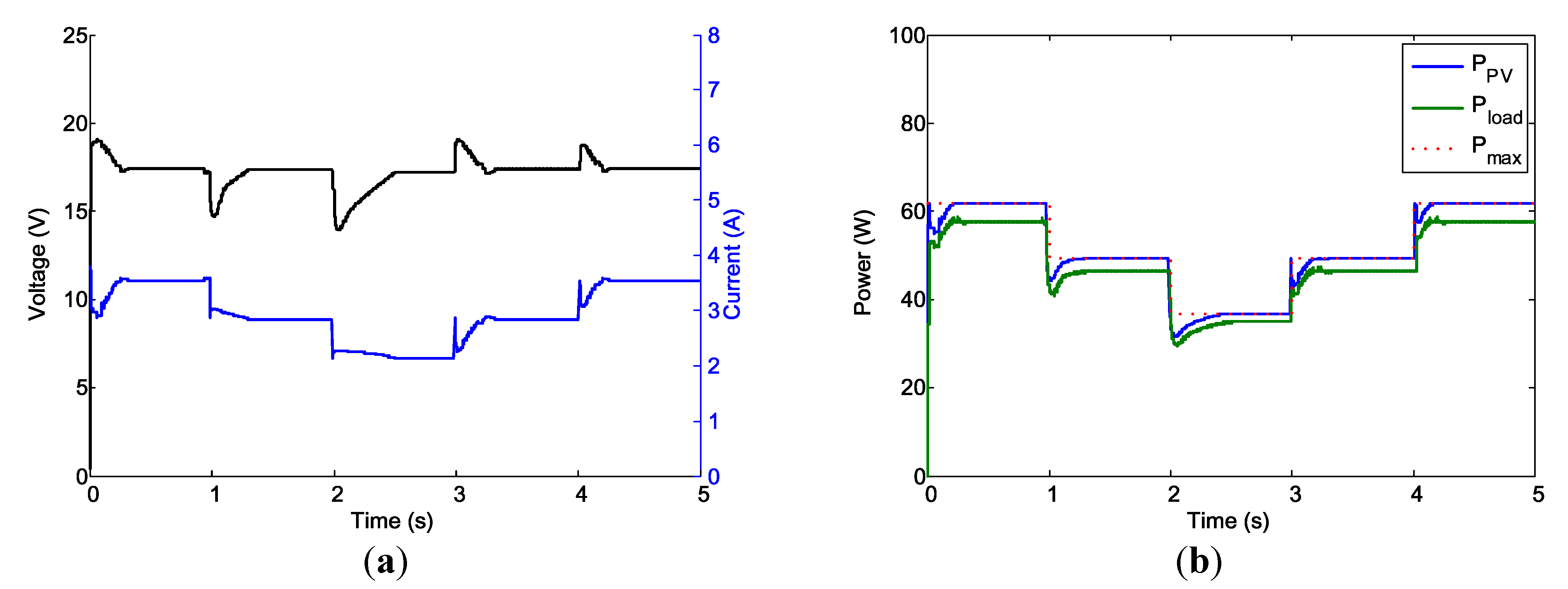Figure 17a shows the voltage and current from the PV model. 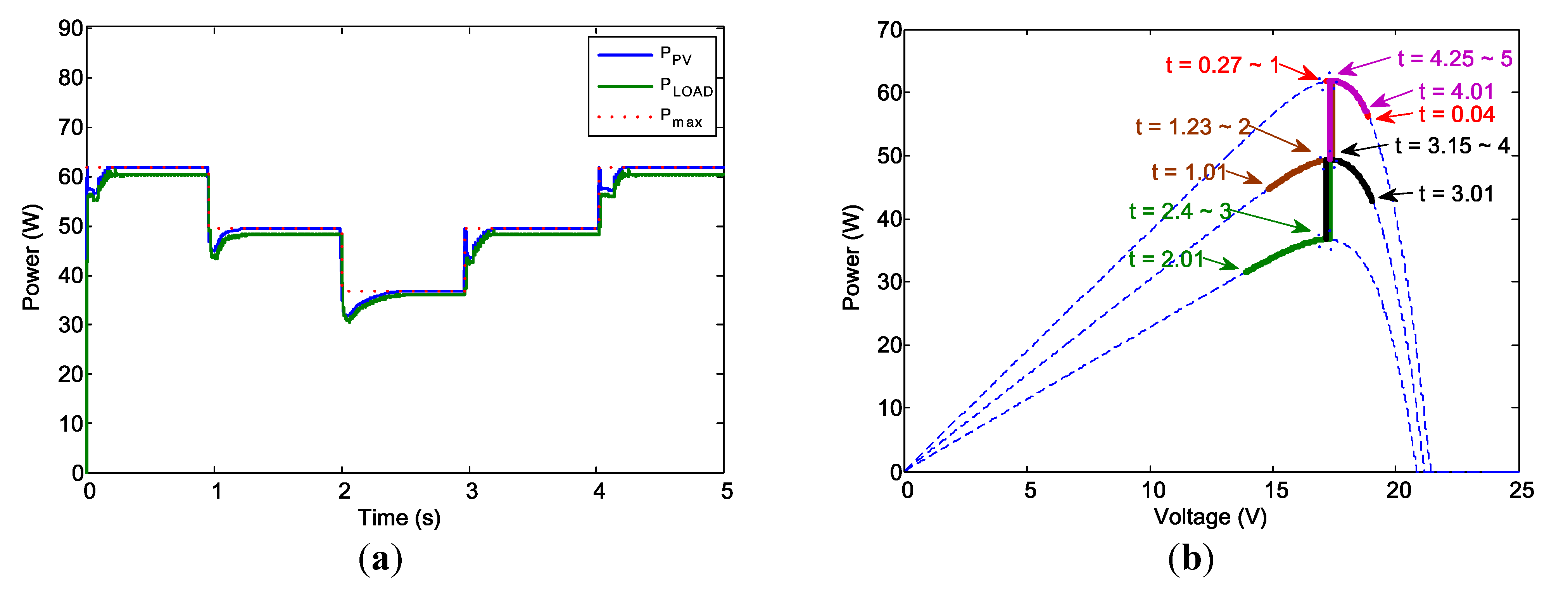The corresponding duty ratio commands are given in Figure 17b. Output power from the PV model and power generated at the load terminal are shown in Figure 18a. Results in Figure 18b are the trajectories of power versus PV voltage during the irradiation variation simulation. The simulation results reveal that maximum power points are almost perfectly reached after short transient.

Figure 17. Circuit simulation for irradiation variations using SEPIC converter. (a) Voltage and current from PV model; (b) Evolution of duty ratio commands.

Figure 17. Circuit simulation for irradiation variations using SEPIC converter. (a) Voltage and current from PV model; (b) Evolution of duty ratio commands.

Figure 18. (a) Power output from PV model and power at the load terminal; (b) Power output from PV model versus PV voltage.

Figure 18. (a) Power output from PV model and power at the load terminal; (b) Power output from PV model versus PV voltage.

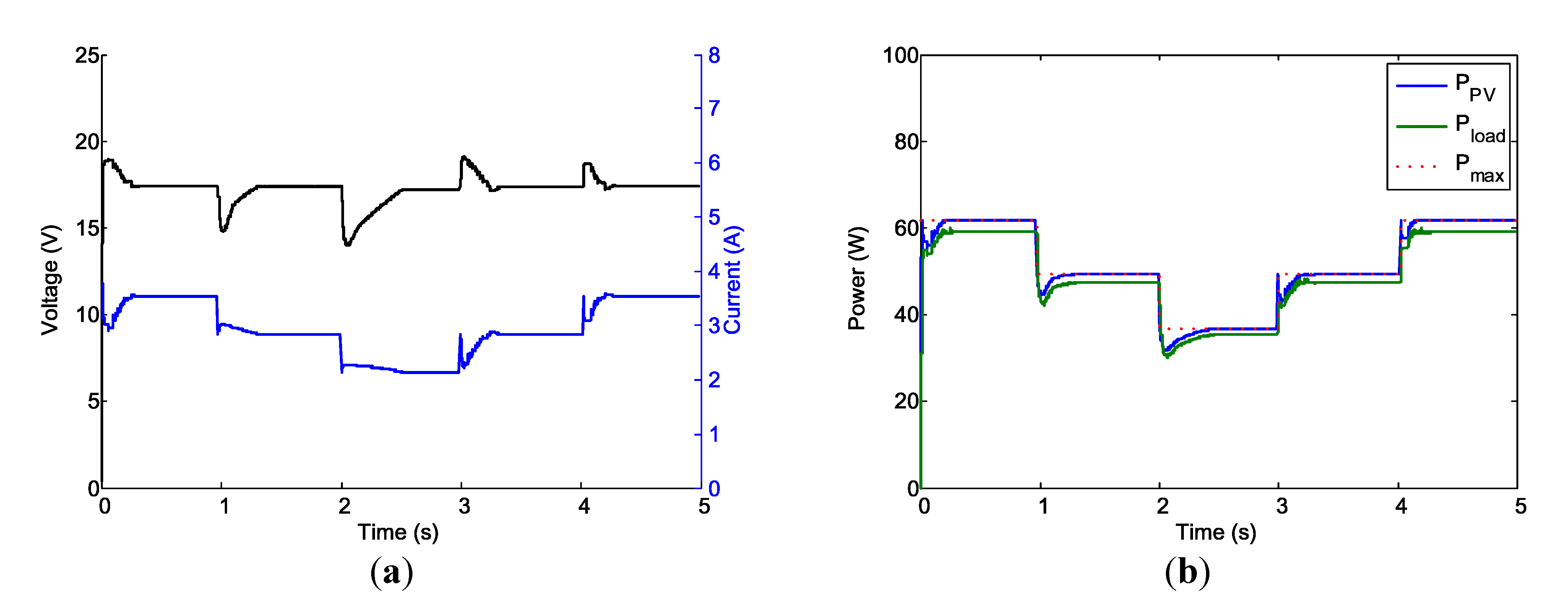
Circuit simulations for irradiation variations using Zeta and four-switch type converters were also conducted. The results are presented in Figure 19 and Figure 20. The results also show that maximum power points are reached.

In summary, we have successfully developed and conducted the circuit simulation for solar power MPPT system using three different buck-boost converter topologies. We almost perfectly reach the maximum power point in all of the simulations.

Figure 19. Circuit simulation for irradiation variations using Zeta converter. (a) Voltage and current from PV model; (b) Power output from PV model and power at the load terminal.

Figure 19. Circuit simulation for irradiation variations using Zeta converter. (a) Voltage and current from PV model; (b) Power output from PV model and power at the load terminal.

Figure 20. Circuit simulation for irradiation variations using four-switch type converter. (a) Voltage and current from PV model; (b) Power output from PV model and power at the load terminal.

Figure 20. Circuit simulation for irradiation variations using four-switch type converter. (a) Voltage and current from PV model; (b) Power output from PV model and power at the load terminal.

7. Conclusions

This paper presents the development of a circuit simulation model for maximum power point tracking (MPPT) evaluation of solar power that involves using different buck-boost converter topologies including SEPIC, Zeta, and four-switch type buck-boost DC/DC converters. The circuit simulation model includes a PV model, a buck-boost converter-based MPPT system, and a fuzzy logic MPPT controller. Circuit simulations for the complete buck-boost converter-based MPPT systems using SEPIC, Zeta, and four-switch type converter topologies were successfully verified in the MATLAB/Simulink PLECS environment.

The circuit simulation framework developed in the paper provides the possibility of investigation and evaluation of a solar power MPPT system without the need of any hardware system and instruments. It is especially useful in the early stage of the development of a solar power management system. It can also be used for evaluating the performance of other power converters and MPPT algorithms.

References

1. International Energy Agency. Technology Roadmap: Solar Photovoltaic Energy; IEA Publications: Paris, France, 2010; Available online: http://www.iea.org/publications/freepublications/publication/pv_roadmap-1.pdf (accessed on 19 February 2014).
2. Tomabechi, K. Energy resources in the future. Energies 2010, 3, 686–695. [Google Scholar] [CrossRef]
3. Weissbach, R.S.; Torres, K.M. A non-inverting buck-boost converter with reduced components using a microcontroller. In Proceedings of the Southeast Conference, Clemson, SC, USA, 30 March–1 April 2001; pp. 79–84.
4. Sahu, B.; Rincon-Mora, G.A. A low voltage, dynamic, noninverting, synchronous buck-boost converter for portable application. IEEE Trans. Power Electron. 2004, 19, 443–452. [Google Scholar] [CrossRef]
5. Gaboriault, M.; Notman, A. A high efficiency, non-inverting, buck-boost DC-DC converter. In Proceedings of IEEE Applied Power Electronics Conference and Exposition, Anaheim, CA, USA, 22–26 February 2004; pp. 1411–1415.
6. Qiao, H.; Zhang, Y.; Yao, Y.; Wei, L. Analysis of buck-boost converter for fuel cell electric vehicles. In Proceedings of IEEE International Conference on Vehicular Electronics and Safety, Beijing, China, 13–15 December 2006; pp. 109–113.
7. Shiau, J.-K.; Ma, C.-W. Li-ion battery charging with a buck-boost power converter for a solar powered battery management system. Energies 2013, 6, 1669–1699. [Google Scholar] [CrossRef]
8. Wu, T.; Chang, C.; Chen, Y. A Fuzzy-logic-controlled single-stage converter for PV-powered lighting system applications. IEEE Trans. Ind. Electron. 2000, 47, 287–296. [Google Scholar] [CrossRef]
9. Alajmi, B.N.; Ahmed, K.H.; Finney, S.J.; Williams, B.W. Fuzzy-logic-control approach of a modified hill-climbing method for maximum power point in microgrid standalone photovoltaic system. IEEE Trans. Power Electron. 2011, 26, 1022–1030. [Google Scholar] [CrossRef]
10. Takun, P.; Kaitwanidvilai, S.; Jettanasen, C. Maximum power point tracking using fuzzy logic control for photovoltaic systems. In Proceedings of the International MutiConference of Engineers and Computer Scientists, Hong Kong, China, 16–18 March 2011.
11. Khateb, A.E.; Rahim, N.A.; Selvaraj, J.; Uddin, M.N. Fuzzy logic controller based SEPIC converter of maximum power point tracking. In Proceedings of IEEE Industry Application Society Annual Meeting,, Las Vegas, NV, USA, 10–11 October 2012; pp. 1–9.
12. Liu, C.-L.; Chiu, Y.-S.; Liu, Y.-H.; Ho, Y.-H.; Huang, S.-S. Optimization of a fuzzy-logic-control-based five-stage battery charger using a fuzzy-based taguchi method. Energies 2013, 6, 3528–3547. [Google Scholar] [CrossRef]
13. Venkatanarayanan, S.; Saravanan, M. Fuzzy logic based PV energy system with SEPIC converter. J. Theor. Appl. Inf. Technol. 2014, 59, 89–95. [Google Scholar]
14. Liu, C.-L.; Chen, J.-H.; Liu, Y.-H.; Yang, Z.-Z. An asymmetrical fuzzy-logic-control-based MPPT algorithm for photovoltaic systems. Energies 2014, 7, 2177–2193. [Google Scholar] [CrossRef]
15. Suntio, T.; Leppaaho, J.; Huusari, J.; Nousiainen, L. Issues on solar-generator interfacing with current-fed MPP-tracking converters. IEEE Trans. Power Electron. 2010, 25, 2409–2419. [Google Scholar] [CrossRef]
16. Nousiainen, L.; Puukko, J.; Maki, A.; Messo, T.; Huusari, J.; Jokipii, J.; Viinamaki, J.; Lobera, D.T.; Valkealahti, S.; Suntio, T. Photovoltaic generator as an input source for power electronic converters. IEEE Trans. Power Electron. 2013, 28, 3028–3038. [Google Scholar] [CrossRef]
17. Walker, G. Evaluating MPPT converter topologies using a MATLAB PV model. J. Electr. Electron. Eng. 2001, 21, 49–55. [Google Scholar]