Hybrid Model Representation of a TLP Including Flexible Topsides in Non-Linear Regular Waves


Abstract
: The rising demand for renewable energy solutions is forcing the established industries to expand and continue evolving. For the wind energy sector, the vast resources in deep sea locations have encouraged research towards the installation of turbines in deeper waters. One of the most promising technologies able to solve this challenge is the floating wind turbine foundation. For the ultimate limit state, where higher order wave loads have a significant influence, a design tool that couples non-linear excitations with structural dynamics is required. To properly describe the behavior of such a structure, a numerical model is proposed and validated by physical test results. The model is applied to a case study of a tension leg platform with a flexible topside mimicking the tower and a lumped mass mimicking the rotor-nacelle assembly. The model is additionally compared to current commercial software, where the need for the coupled higher order dynamics proposed in this paper becomes evident.1. Introduction
The Horizon2020 call [1] of the EU states explicitly that innovative substructure concepts, including floating platforms, are needed for water depths beyond 50 m, in order to push the development of competitive low carbon energy generation. One focus is to reduce the overall project risks. However, such project risks can only be accounted for or avoided if known and if their impact can be assessed by applicable tools. Conventional tools used in the oil and gas (O&G) industry for the assessment of the extreme event response of floating structures neglect two important aspects, making them non-conservative when used for floating offshore wind turbines (FOWT). Considering that the offshore wind industry intends to install floating structures at a much shallower water depth than the offshore O&G industry, i.e., in the order of 50 m, a first or second order wave theory approach might not be sufficient to describe realistic wave shapes. Therefore, a higher order wave theory seems necessary. Furthermore, wind turbines are dynamically sensitive structures. Even while the floating part can be considered more or less rigid, the flexibility of the slender tower supporting a heavy rotor-nacelle assembly (RNA) influences the structure’s response significantly. The significance of this is highlighted in the recently released DNVoffshore standard, J103 [2], for the design of floating wind turbine structures, which specifically addresses the importance of the flexibility of the tower for the correct simulation of pitch and roll motions. The relation between tower flexibility and response amplitude operator (RAO) shift has been pointed out by Matha [3] in recent years. A numerical model of a tension leg platform (TLP) was compared against measured responses from tests carried out within the DeepCwind framework in [4]. Besides decay tests and wind wave loading, their TLP was exposed to a number of regular waves. The software, as well as the tests considered linear waves, and a reasonable agreement was found. A numerical comparison to the physical model tests of the DeepCwind TLP was performed in [5]. An underestimation of the spectral amplitudes around the natural pitch frequency in regular waves without wind was found. It was suggested that this might be due to the harmonics in the physical wave realization coinciding with the pitch natural frequency. The current work investigates if it is possible to consider these effects by including the viscous wave excitation from higher wave harmonics for the surface-piercing, drag-dominated structural part.
In summary, the current work assesses how well a hybrid model, consisting of a linear potential theory wave excitation and viscous force non-linear wave excitation, can predict key parameters of an FOWT in intermediate water depths. Such environments are common in ultimate limit state analysis (ULS), and often, wave shapes deviate from the first or second order description. As this violates the linear theory, the hybrid model is, in the current work, compared to observations from wave-tank tests. The general problem was two-fold; the hybrid model should be able to simulate the behavior of a tethered floater exposed to non-linear waves, while also accommodating the influences of non-rigid topsides. The hybrid model is an extendable research tool forming the basis of an in-house development. Further benchmarking against available tools at a later stage is planned. It is essential to note that the work is not a design verification, but a tool validation. Even though the full tendon length could be modeled due to a deep section in the wave basin, the structure originally designed for a 100-m water depth was exposed to waves generated in approximately a 60-m water depth. This caused the waves to become non-linear and, hence, allowed the assessment of the performance of a hybrid model, including non-linear viscous wave force excitation.
2. Methods
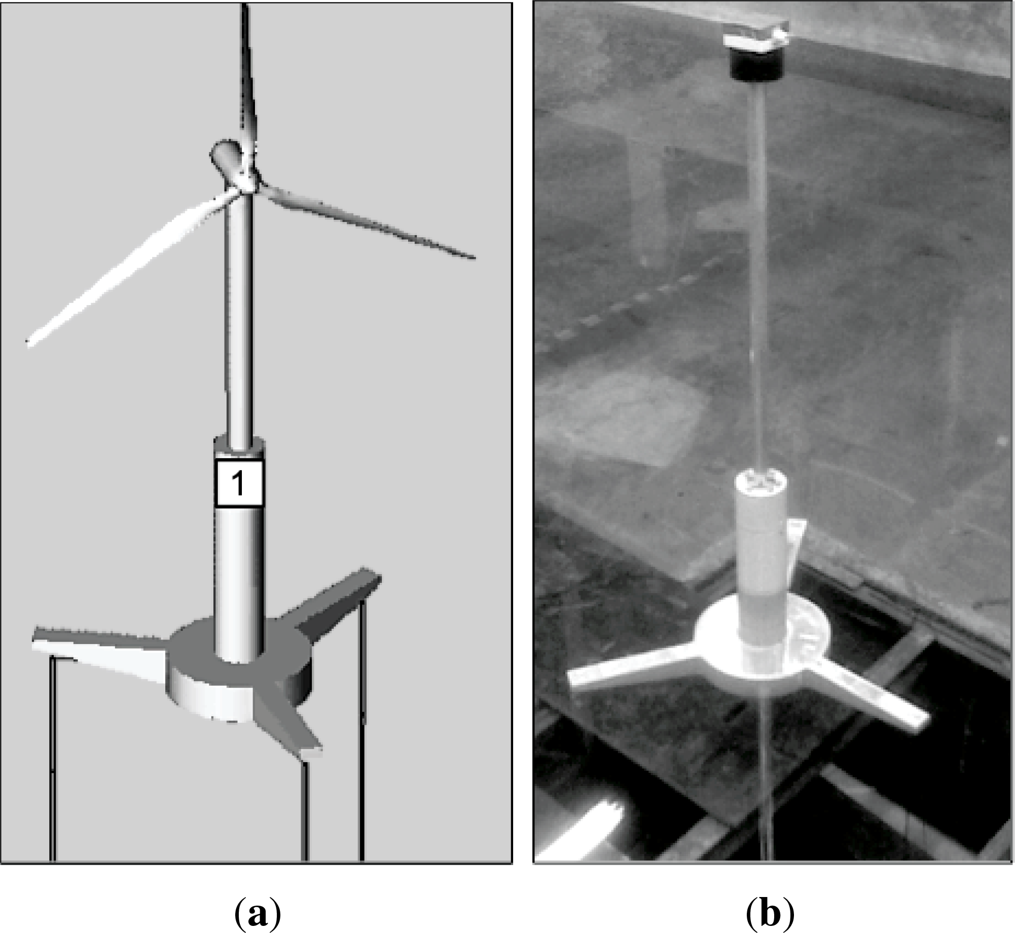
The scope of this section is to detail the assumptions and methodologies used throughout the work. The objective of this study is to implement a numerical model of a floating wind turbine mounted on an industry-inspired TLP. The numerical model will be exposed to regular, non-linear extreme waves representing ultimate limit state (ULS) conditions. DNV J103 [2] suggests this option to assess the behavior of an offshore wind turbine structure in design conditions. The numerical model will then be validated against experimental tests. The tests were conducted in the 3D wave basin at Aalborg University on a 1:80 scale model; see Figure 1. A detailed description of the set-up and results can be found in [6].
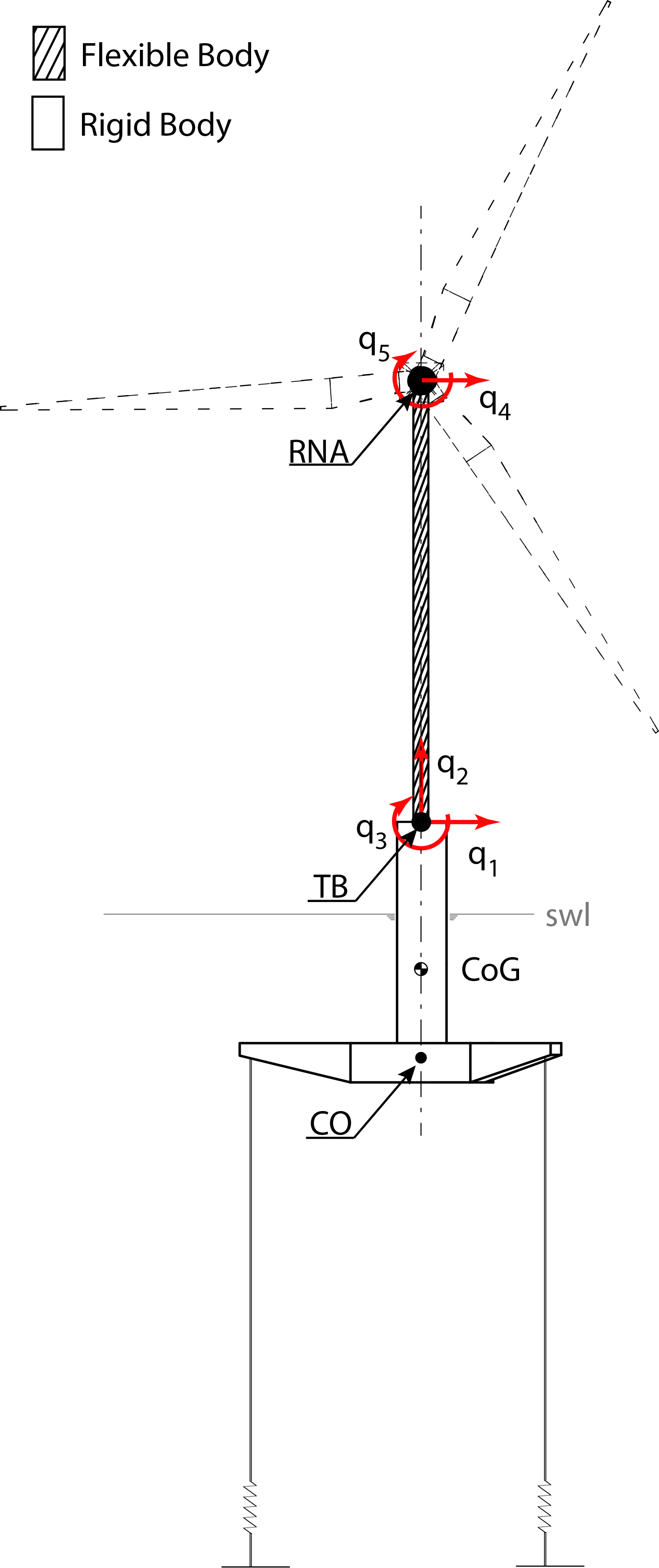
Figure 2 shows a sketch of the system under investigation, where the main elements are the TLP substructure (with the associated station-keeping system), the tower and the RNA. q is the 5 degrees of freedom (DOF) displacement vector, and q1 and q2 are the surge and heave motion of the structure, pointing in positive x and z, respectively. TB is the tower bottom, i.e., the connection point between tower and substructure. swl is the still water line. CoG is the center of gravity of the TLP. CO is the elevation of the mooring attachment point projected onto the centerline of the structure.
Although both wave and wind loads excite the motion of the structure, the current validation focuses on the hydrodynamic response only. It is important to note that in actual ULS conditions, the wind load on the tower, as well as on the blades can become important during fault conditions.
Considering the construction method of the floater [6], it seems sensible to assume it to be rigid. However, as already mentioned in the previous section, the influence of tower flexibility on the dynamic response of the total structure cannot be neglected [3]. Therefore, the substructure model will be coupled with a flexible beam element connecting the RNA to the rigid substructure.
The substructure has trilateral symmetry about a vertical axis passing through its center. The dynamic response is studied in long crested, i.e., 2D, incident waves, as has been done in the physical model test. The simplified model and the definition of the relative coordinate system are represented in Figure 2.
2.1. Numerical Model of the Substructure
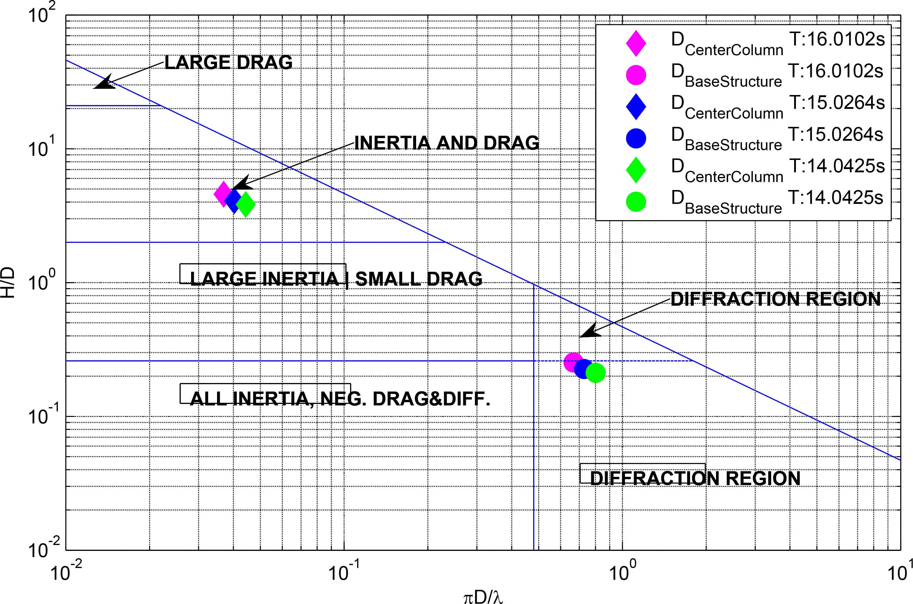
The model will be based on a boundary integral equation method (BIEM) solution with additional hydrodynamic viscous drag terms according to Morison’s equation. This approach is believed to be more time efficient than complex numerical techniques, e.g., computational fluid dynamics. The need for an extra dissipative term related to viscous effects in the boundary layer is supported by the results of a non-dimensional analysis of the structure. Figure 3 shows that, based on the non-dimensional ratio between inertial and viscous loads, the flow regime changes along the vertical axis of the structure, and consequently, the use of BIEM plus a viscous drag term becomes necessary. Hence, the wave-body interaction is decomposed into four contributions:
Wave excitation force: BIEM;
Viscous drag forces;
Radiation force;
Hydrostatic force.
2.1.1. Wave Excitation Forces from Potential Flow
Wave excitation forces (Fex) are defined as the loads exerted on a submerged structure held in equilibrium position in waves.
The total excitation forces are expressed as a summation of the Froude–Krylov forces ( ) and the diffraction forces ( ). The index i represents the i-th degree of freedom. The Froude–Krylov forces are due to the undisturbed incident waves, while the diffraction forces are related to the modified wave field generated by the structure. The forces are obtained from the integration of the linearized dynamic pressure distribution over the mean wetted surface. The complex frequency coefficients, describing the summation of those two forces, are obtained from the solution of the boundary integral equation problem using the commercial software, ANSYS AQWA [8]. The wave excitation force vector (Fex) is assessed in the time domain by convolution of the non-causal impulse response function (IRF) with the surface elevation time series for each DOF.
2.1.2. Viscous Drag Forces
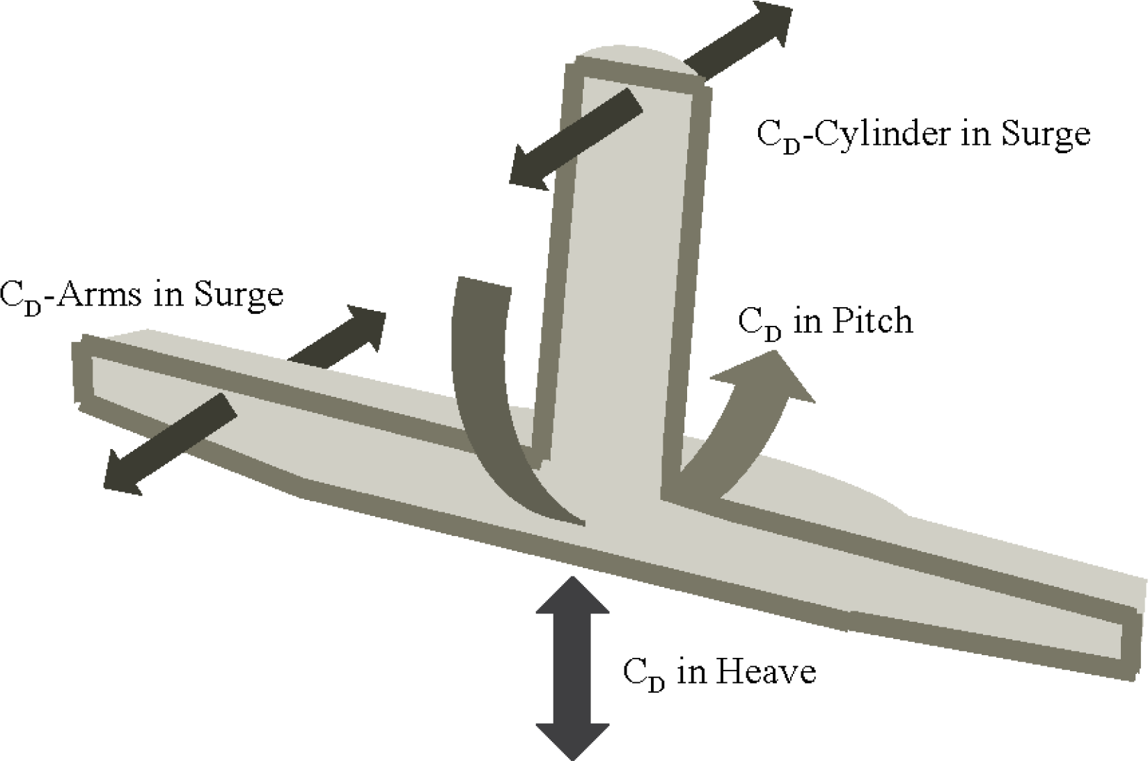
Viscous energy dissipation, i.e., flow separation, is likely to influence the motion of the system, due to the different flow regimes along the structure. This can be seen as an additional excitation force, as the wave particle velocity is likely to be higher than the body velocity, especially for the surface piercing part. The i-th viscous drag force ( ) used in the model is defined in Equation (1), where i refers to the drag force component, as shown in Figure 4.
2.1.3. Radiation Forces
The radiation force is the load exerted by the moving body in otherwise calm water. The total radiation load is composed of a part proportional to the acceleration of the body (added mass) and a part proportional to the velocity (radiation damping) of it. The time domain model is represented by the so-called fluid memory terms (IRF) and the matrix of added mass at infinite frequency. This term is related to the convergence of the integral, as detailed in [9]. Although the same convolution approach can be used to evaluate the radiation force vector (Frad), it benefits the implementation to approximate the frequency response function by a system of first order ODEs. As presented in [9,10], a fifth or lower order system is enough to model a smooth response, as for the presented structure. The state space approximation of the radiation problem is obtained from a least squares fit of the radiation frequency response function. The freeware marine toolbox has been used for this purpose [10]. The selected model order is three.
2.1.4. Hydrostatic Forces
The hydrostatic stiffness matrix of the rigid body is obtained from ANSYS AQWA.
2.1.5. Numerical Model of the Station-Keeping System
A mooring system is required by every floating offshore structure for station-keeping purposes. Furthermore, for TLP-like structures, the mooring system compensates for the intrinsic instability of the system, providing a global positive restoring coefficient. For slender bodies, such as the tendons, it is possible to assume that the major load contributions come from stiffness along the axis of symmetry and from drag in the perpendicular direction. Nevertheless, due to the small cross-sectional area of the tendons used in the lab, it is possible to assume that their drag contribution is negligible, thus the mooring force reduces to a force proportional to the linear extension of the mooring cable. The mooring force Fm is detailed in the following equation:
2.1.6. Numerical Model of the Tower
In order to include the dynamic influence of a flexible tower into the model, a standard linear elastic Euler–Bernoulli beam element with four degrees of freedom (q1, q3, q4, q5) has been used, where the beam top end is connected to a lumped mass representing the RNA.
Only the first mode shape for each degree of freedom is used as a consequence of the ratio between lumped mass over beam mass. The resultant model of the tower has five DOFs: the surge (q1, q4) plus pitch (q3, q5) of the bottom and top, respectively, and a shared heave motion (q2); see Figure 2. Additionally, it is fully described by the mass and stiffness matrix. In addition to those matrices, a damping matrix is implemented to simulate the damping from the topside structure. Rayleigh damping is used, and damping ratios are determined by decay tests. Definitions of the general mass, damping and stiffness matrices are given in [11], together with a comprehensive description of their derivation.
2.1.7. Combined Model
The above-mentioned loads are then assembled in a global system, where the equation of motion is given by:
The global mass and stiffness matrices are obtained from the summation of the sub-structure and tower matrices in the shared DOFs to ensure the dynamic coupling of the two bodies. The equation of motion is solved by the ODE45algorithm implemented in MATLAB [12].
2.2. Wave Model
In order to simulate ULS conditions, a proper wave model is needed. In deep water, the ULS waves can be represented with linear or non-linear waves of small order, such as first or second order Stokes waves. For severe waves in intermediate to shallow water, a higher order solution is needed. Based on the best fit with the experimentally observed wave shapes, a 30th order stream function wave theory is adopted [13]. Wave kinematics and surface elevations are obtained and subsequently applied in the hybrid model. Table 1 shows the applied regular wave parameters in the prototype scale.
3. Results
The numerical results and their comparison with prior experimental measurements are presented in this section. In the first part, the model details are given. In the second part, the code-to-code and the code-to-experiment comparisons are presented. Three different stiffness set-ups of the hybrid model are used: very stiff, stiff and flexible; the first one is used in the code-to-code comparison and the other two in the code-to-experiment comparison. In both cases, the comparison is divided into two steps: first, the decay test response is presented, followed by the wave response in ULS conditions. The time series will have a predefined and constant color map:
Red line: flexible model;
Blue line: stiff model;
Green line: very stiff/quasi-rigid model;
Black line: reference signal (ANSYS AQWA and/or experimental results).
3.1. Parameters Definition
The prototype is a three-armed TLP structure, with an approximate total weight, including tower and turbine, of around 2,000 t, installed at a water depth of 100 m [6]. The topside mass is roughly 40% of the substructure mass. In order to include the viscous drag, it was assumed that four different viscous force contributions were sufficient. Figure 4 illustrates the idealized viscous drag contributions that are implemented in the model. These forces were included using the instantaneous relative velocities between body and water particle at specific locations. The CD values for cylinders and for heave motions agree with common industry standards. For the heave motion, the obtained values were constant and were typical for separated flows at small KC numbers for angular parts [14]. Being a common practice in the offshore wind industry, the CD values for the cylinder are calculated as a function of maximum undisturbed Reynolds number and maximum undisturbed KC number. More details can be found in [15].
Table 2 shows the applied drag coefficients. A KC relationship for the CD in pitch was iteratively fitted and resulted in values similar to the ones in heave. The drag coefficient values for the projected area of the arms were iteratively fitted, as well. It is obvious that the CD approximations for the lower part of the structure have been tailored to the structural layout and the respective assumptions. The estimated CD value for the surface piercing cylinder in the surge direction, as well as the CD in the heave and pitch direction agree well with values that can be found in the literature [14,16].
3.2. Code-to-Code Validation
In order to validate the model, a code-to-code comparison with the commercial software, ANSYS AQWA, was carried out first. The results are presented hereafter for both the decay test and wave induced motion. The study focuses on the pitch response, being the one most affected by the tower flexibility, but results for the other DOFs are also presented in order to verify the response model. Since ANSYS AQWA models the entire structure as one rigid body, this can be used as a benchmark case to validate the hybrid model. In the hybrid model, the substructure is rigid, as well, and by applying a tower stiffness, EI, of orders of magnitude larger than the physical one, quasi-rigid body behavior is emulated.
3.2.1. Decay Test
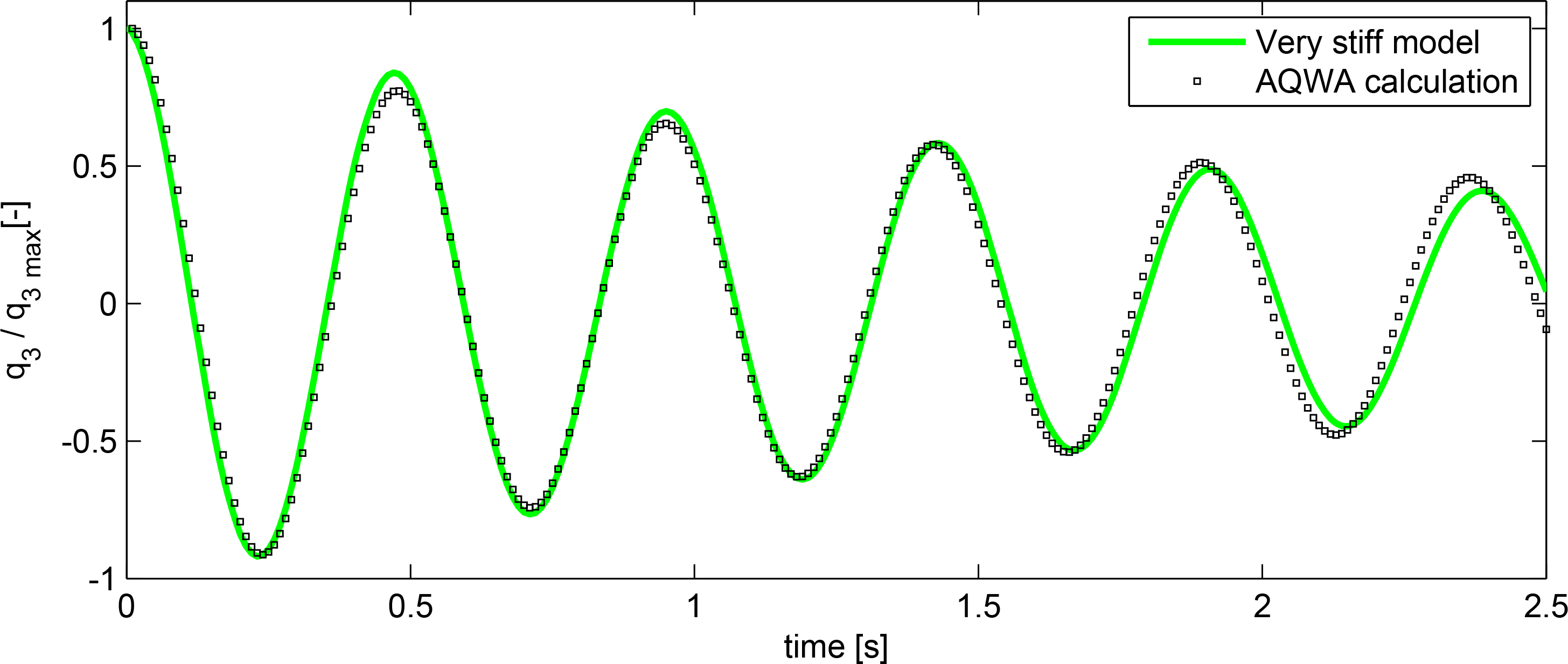
Figure 5 shows the time series comparison between the rigid body response predicted by ANSYS AQWA and the hybrid model. The natural frequency of the rigid body motion predicted by the hybrid model is 2.05 Hz, where ANSYS AQWA predicts 2.10 Hz.
3.2.2. Regular Waves
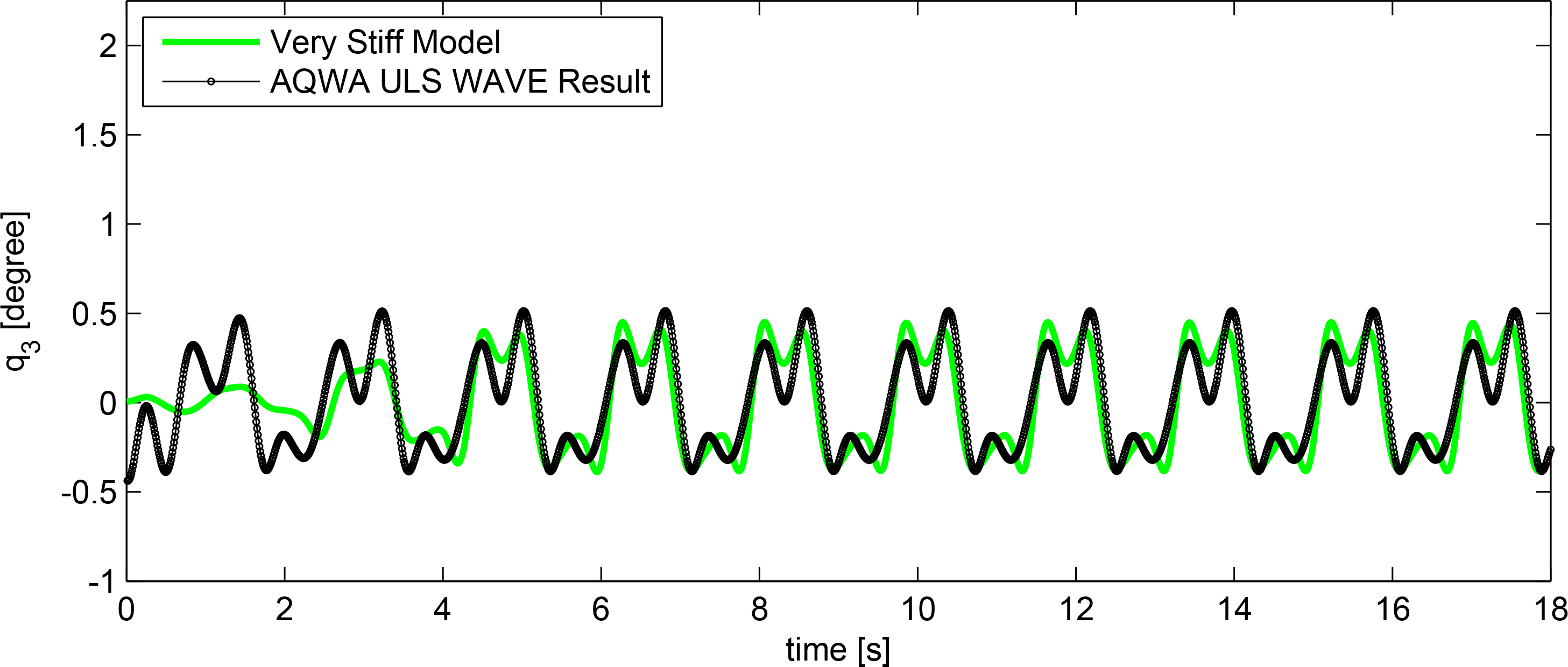
A ULS design load case is generated with ANSYS AQWA, simulating rigid body behavior. The software generates second order regular Stoke waves. In order to mimic the physical test environment, the water depth matched the wave generation water depth in the wave tank, which, in turn, matched the water depth used in the numerical model for the generation of the stream function wave. Figure 6 shows the obtained results, and a good match is observed. The waves in the hybrid model are ramped for all cases, explaining the comparison convergence.
3.3. Physical Model Validation
Once a qualitative analysis of the hybrid model’s capability was complete, the hybrid model was validated against experimental data. As previously mentioned, two different structural stiffness configurations form the basis of comparison, namely the stiff and flexible model [6]. The response will be evaluated in TB, as defined in Figure 2. TB has been selected as the point of comparison due to sensor location in the experimental setup. Consequently, only a single transformation from CoG to TB within the numerical model is required.
3.3.1. Decay Test
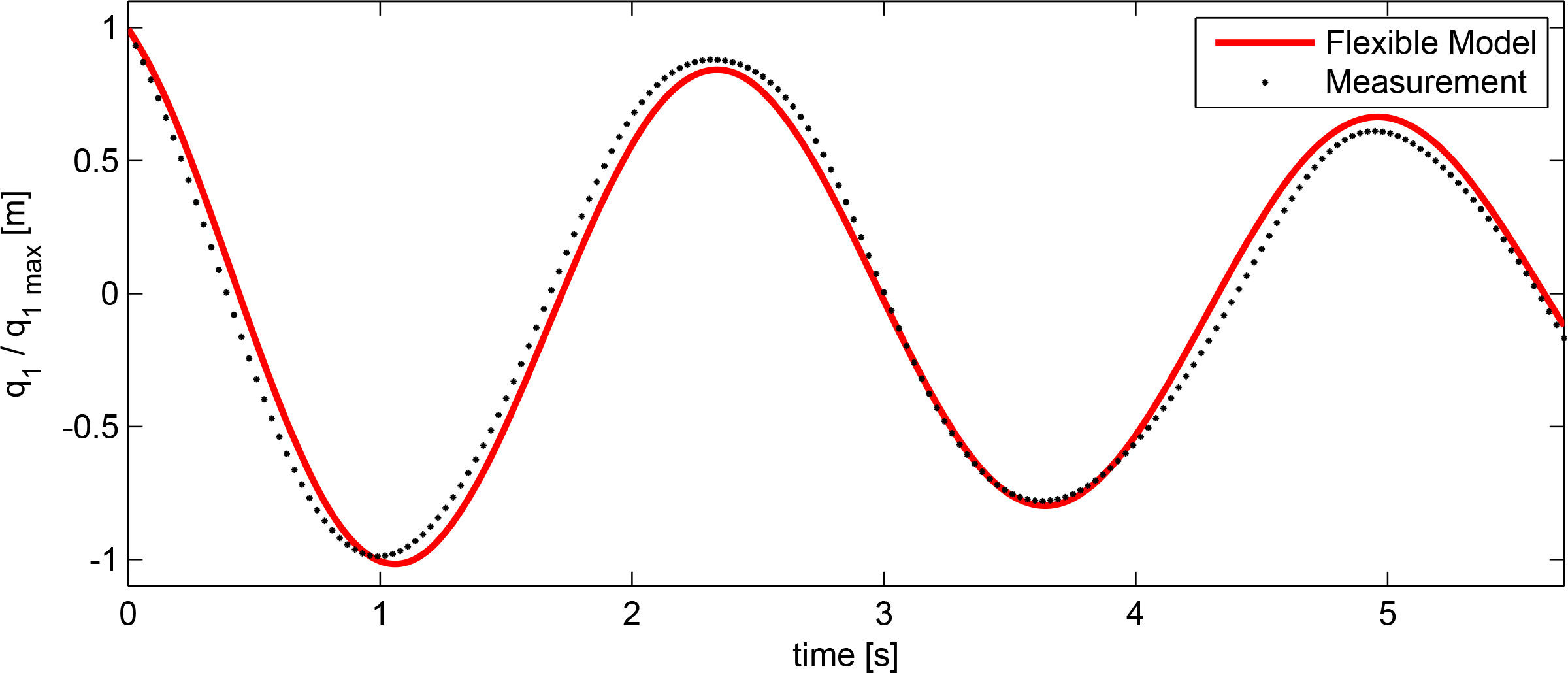
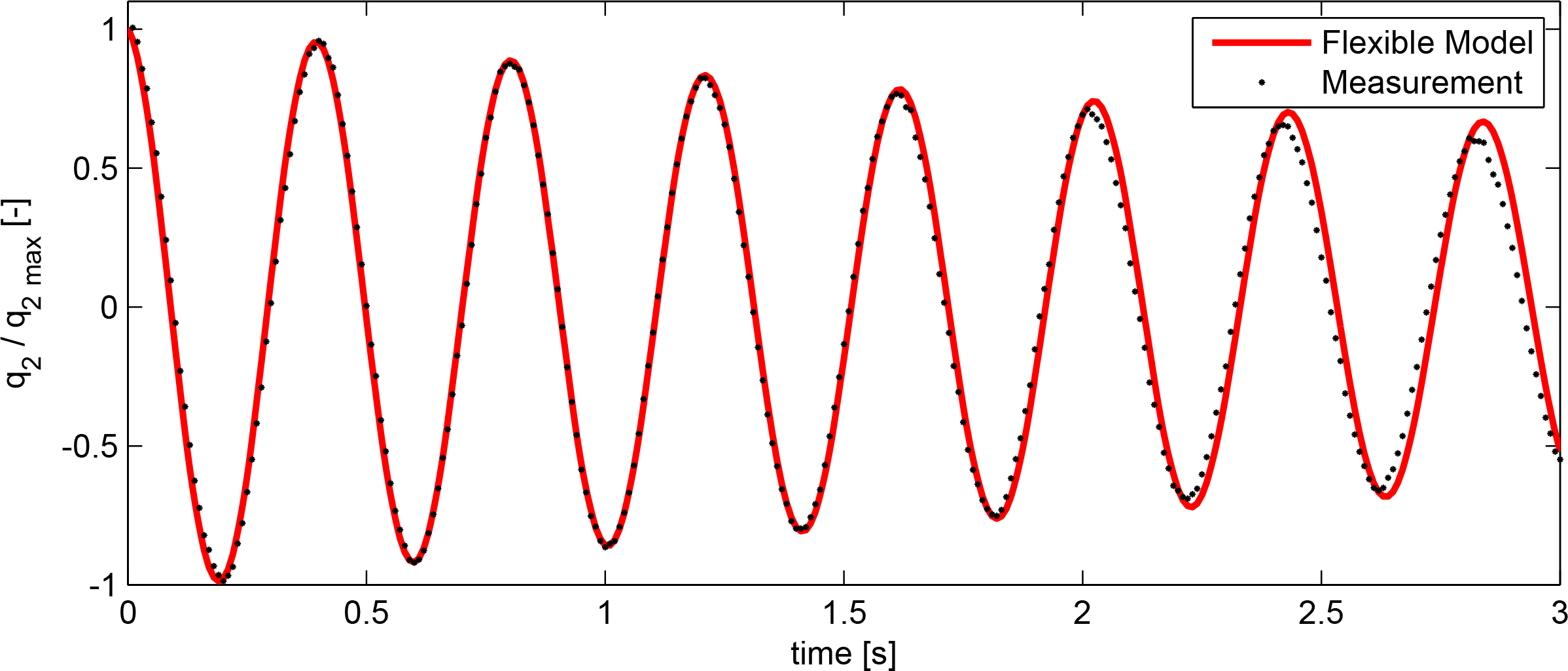
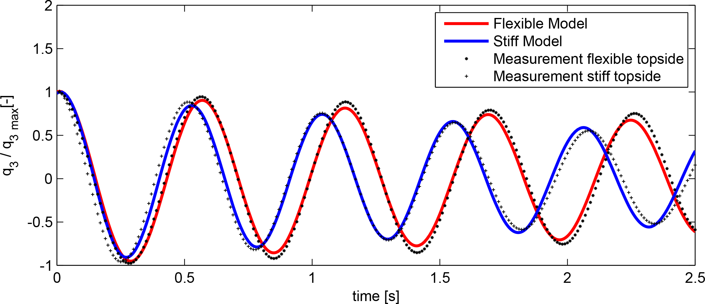
The responses in surge and heave for the flexible tower system are shown in Figures 7 and 8, respectively. Figure 9 shows the pitch response comparison between flexible and rigid tower lay-outs, for both experimental and numerical models. Only the flexible model is used for the comparison of the decay in surge and heave, since the period in surge is orders of magnitude larger than that of the natural frequency of the tower bending mode, making the two models indistinguishable. This is also the case for the heave decay, since the axial stiffness of the tower is orders of magnitude higher than the vertical stiffness of the foundation and mooring.
3.3.2. Regular Waves
The numerical model was subsequently applied to three different wave conditions in accordance with the three largest sea states used in the physical model tests. Example time series plots for the upper and lower bounds, i.e., flexible topside response to the highest wave and stiff topside response to the lowest wave, are given in Figures 10 and 11.
4. Discussion
In order to gain an understanding of the model quality when compared with experimental results, cross-correlation coefficients and ratios between maximum and minimum values have been obtained, excluding the initial effects from the ramping up; see Tables 3 and 4. The correlation coefficients varied between 80%–96%, with an average of 88%. The ratios between the respective predicted minimum values and observed values showed good agreement. The maximum deviation was an 18% underestimation of the numerical model. An average deviation of 8% was found.
To obtain a better understanding of the force contributions, the pitch excitation moment was split into its single components for one period; see Figure 12. It is obvious that the horizontal drag force acting on the cylinder is the dominating load, i.e., the combined total moment is dominated by the kinematics above the still water level impacting on the surface piercing part. The overturning moment is much larger than the moment induced by the loads acting on the lower part of the structure. The latter is, in fact, opposite, as the horizontal velocities are acting below the point of rotation. The diffractive part of the moment dominates the negative peak when the horizontal velocity components of the wave kinematics are close to zero. Hence, neither a pure potential flow approach nor a pure viscous force approach would be able to deliver the same degree of fit.
The hybrid model performs well when looking at the power spectra of the pitch decay responses; see Figure 13. Only a minor deviation is found for the very stiff model compared to the ANSYS AQWA response. For the regular wave pitch response spectra, the results are two-fold; see Figure 14. It becomes clear that the stream function wave cannot fully reproduce the laboratory waves, and in particular, the very high frequency components are underestimated. However, the influence on the structural response is negligible. The third order component is close to the pitch eigenfrequency of all structural layouts, and consequently, the dynamic amplification due to the flexibility of the topside becomes evident. The hybrid model matches the observed pitch response, whereas the very stiff model matches the results from the ANSYS AQWA model. Room for improvement can be found at the second order component; unlike the ANSYS AQWA model, the hybrid model lacks the inclusion of the second order sum frequency excitation force, explaining why both the flexible and very stiff models underestimate the responses, while the ANSYS AQWA model shows a better match.
5. Conclusions
Non-linear waves are assumed to be relevant in the ULS analysis of FOWTs installed close to the minimum target water depth of ∼50 m. The intention was to set up a resource-efficient tool, able to satisfactorily approximate pitch motions of a dynamically-sensitive FOWT resulting from a nonlinear wave impact. As a numerical experiment, a hybrid model was developed, including linear potential theory forces and non-linear hydrodynamic viscous forces. The potential forces act thereby on the large volume part of the structure, whereas the viscous forces act on the cylindrical surface piercing part of the structure. Due to the violation of the potential flow approximations induced by wave non-linearity, the hybrid model needs to be validated by experimental tests. The CD values applied in the hybrid model are used as tuning parameters. Considering that these are in sensible ranges, the overall match between the observations and the hybrid model is very good. To the authors knowledge, this is the first time a mildly-nonlinear approach has been assessed, comparing measured pitch responses to observed pitch responses excited by non-linear waves based on stream function theory. The term mildly-nonlinear describes the combination of linear radiation and wave scattering combined with additional non-linear terms, assuming small body motions. It was shown that the viscous drag contributions are an essential part of the response for the investigated structure, and it seems sensible to include those effects, as well, in subsequent irregular wave response analysis. Additionally, a code-to-code comparison was carried out and served as the performance verification for non-flexible topside configurations. It was shown that the hybrid model can be adopted to deliver more than satisfying results for different wave steepness values and different topside flexibilities. The model is thereby able to:
Include the effects of regular, non-linear waves on an FOWT TLP structure;
Include the effects of the dynamically-sensitive topside on the pitch response of an FOWT.
Comparing the maximum pitch values obtained by the rigid body simulation to those of the flexible topside simulation, the impact of the rigid body assumption becomes evident. Even though this appeared to be very structure specific, it underlines the importance of the correct implementation and furthermore proves that the rigid body assumption inherited from the O&G industry is not valid for FOWTs. It was not expected to obtain perfect fits, due to the complexity of the system and due to the simplifications. A higher fidelity model could be achieved by inclusion of the nonlinear Froude–Krylov force. When simulating irregular waves, second order diffraction forces might become relevant. However, the non-linear viscous contributions are expected to be of the same or higher significance, especially in severe seas for surface piercing parts, which are drag dominated. Considering the lateral extent of the structure, an integration of the instantaneous drag contribution over the wetted surface might lead to further improvement. However, the results already showed good agreement with the measured data. It is thereby concluded that the applied methodology is robust enough to be developed further. A natural next step is the assessment of key responses in irregular waves. Even though the general approach seems valid, a current limitation, and, therefore, incentive for future work, is the specific applicability of the model. Exchanging the potential flow coefficients is not a major challenge; however, the current drag coefficient implementation and the current mooring model makes the model case specific. Further development work, in order to make the model more generally applicable, i.e., acceptable for different substructures and mooring configurations, is consequently planned.
Acknowledgments
The early stage PelaStar design by THE GLOSTEN ASSOCIATESwas the genesis of the subject TLP. Their contribution to the project is gratefully acknowledged. The access to the wave laboratory of Aalborg University and the support by Aalborg University’s staff provided an invaluable contribution.
Author Contributions
This work was planned and drafted by the C. Wehmeyer. The key methodology and subsequently implementation of the numerical model was done by C. Wehmeyer, however with invaluable input from the co-authors. The relevant experimental tests have been shared between F. Ferri and C. Wehmeyer. The contributions and the working atmosphere during the paper development is greatly appreciated.
Conflicts of Interest
The authors declare no conflict of interest.
References
- Call for Competitive Low-Carbon Energy; Technical Report H2020-LCE-2014-1; European Comission: Brussels, Belgium; 11; December; 2013.
- Design of Floating Wind Turbine Structures; Offshore Standard DNV-OS-J103; Det Norske Veritas AS: Hovik, Norway; June; 2013.
- Matha, D. Model Development and Loads Analysis of an Offshore Wind Turbine on a Tension Leg Platform, With a Comparison to Other Floating Turbine Concepts; Subcontract Report NREL/SR-500-45891; National Renewable Energy Laboratory: Golden, CO, USA; February; 2010. [Google Scholar]
- Stewart, G.M.; Lackner, M.A.; Roberton, A.; Jonkman, J.; Goupee, A.J. Calibration and validation of a FAST floating wind turbine model of the deepwind scaled tension-leg platform. In Proceedings of the 22nd International Offshore and Polar Engineering Conference (ISOPE), Rhodes, Greece, 17–22 June 2012.
- Prowell, I.; Robertson, A.; Jonkman, J.; Stewart, G.M.; Goupee, A.J. Numerical prediction of experimentally observed behavior of a scale-model of an offshore wind turbine supported by a tension-leg platform. In Proceedings of the Offshore Technology Conference, Houston, TX, USA, 6–9 May 2013.
- Wehmeyer, C.; Ferri, F.; Skourup, J.; Frigaard, P. Experimental Study of an Offshore Wind Turbine TLP in ULS Conditions. Proceedings of the Twenty-third (2013) International Offshore and Polar Engineering, Anchorage, AK, USA, 30 June–5 July 2013.
- Chakrabarti, S.K. Hydrodynamics of Offshore Structures; WIT Press: Southampton, UK, 1987. [Google Scholar]
- ANSYS AQWA; Version 15.0; ANSYS, Inc.: Canonsburg, PA, USA; November; 2013.
- Yu, Z.; Falnes, J. State-space modelling of a vertical cylinder in heave. Appl. Ocean Res 1995, 17, 265–275. [Google Scholar]
- Perez, T.; Fossen, T.I. A Matlab Toolbox for Parametric Identification of Radiation-Force Models of Ships and Offshore Structures. Model. Identif. Control: Nor. Res. Bull 2009, 30, 1–15. [Google Scholar]
- Clough, R.W.; Penzien, J. Dynamics of Structures; Civil Engineering Series; McGraw-Hill Education: New York, NY, USA, 1993. [Google Scholar]
- MATLAB; Version 7.13.0.564 (R2011b); The MathWorks Inc: Natick, MA, USA, 2011.
- Dean, R.G.; Dalrymple, R.A. Water Wave Mechanics for Engineers and Scientists; Advanced Series on Ocean Engineering-Vol2; World Scientific: Singapore, 1991. [Google Scholar]
- Faltinsen, O. Sea Loads on Ships and Offshore Structures; Cambridge Ocean Technology Series; Cambridge University Press: Cambridge, UK, 1993. [Google Scholar]
- Design of Offshore Wind Turbine Structures; Offshore Standard DNV-OS-J101; Det Norske Veritas AS: Hovik, Norway; October; 2007.
- Sumer, B.M.; Fredsøe, J. Hydrodynamics around Cylindrical Structures; Advanced Series on Ocean Engineering, V.12; World Scientific: Singapore, 1997. [Google Scholar]


| Wave Parameters | Run 18 | Run 17 | Run 16 |
|---|---|---|---|
| Hmax (m) | 17.2 | 15.2 | 14.8 |
| Tmax (s) | 16.0 | 15.0 | 14.0 |
| Direction | Structure part | CD |
|---|---|---|
| Surge | Arms | 1.1 |
| Surge | Cylinder | 1.8 |
| Pitch | Base disc + arms | 0.3 KC |
| Heave | Base disc + arms | 3.3 |
| Flexible Model | Exp. | Num. | Exp. | Num. | Exp. | Num. |
|---|---|---|---|---|---|---|
| Run Number | 18 | 17 | 16 | |||
| Hmax (m) | 0.215 | 0.190 | 0.185 | |||
| Tmax (s) | 1.79 | 1.68 | 1.57 | |||
| Min (degree) | −0.945 | −0.993 | −0.890 | −0.857 | −0.830 | −0.747 |
| Max (degree) | 0.993 | 1.036 | 0.997 | 0.939 | 0.820 | 0.785 |
| Min Ratio (−) | 0.95 | 1.04 | 1.11 | |||
| Max Ratio (−) | 0.96 | 1.06 | 1.04 | |||
| Correlation Coeff. (%) | 92 | 80 | 82 | |||
| Stiff Model | Exp. | Num. | Exp. | Num. | Exp. | Num. |
|---|---|---|---|---|---|---|
| Run Number | 18 | 17 | 16 | |||
| Hmax (m) | 0.215 | 0.190 | 0.185 | |||
| Tmax (s) | 1.79 | 1.68 | 1.57 | |||
| Min (degree) | −0.654 | −0.792 | −0.797 | −0.730 | −0.792 | −0.740 |
| Max (degree) | 0.814 | 0.883 | 0.945 | 0.803 | 0.868 | 0.799 |
| Min Ratio (−) | 0.83 | 1.09 | 1.07 | |||
| Max Ratio (−) | 0.92 | 1.18 | 1.09 | |||
| Correlation Coeff. (%) | 86 | 95 | 95 | |||
© 2014 by the authors; licensee MDPI, Basel, Switzerland This article is an open access article distributed under the terms and conditions of the Creative Commons Attribution license (http://creativecommons.org/licenses/by/3.0/).
Share and Cite
Wehmeyer, C.; Ferri, F.; Andersen, M.T.; Pedersen, R.R. Hybrid Model Representation of a TLP Including Flexible Topsides in Non-Linear Regular Waves. Energies 2014, 7, 5047-5064. https://doi.org/10.3390/en7085047
Wehmeyer C, Ferri F, Andersen MT, Pedersen RR. Hybrid Model Representation of a TLP Including Flexible Topsides in Non-Linear Regular Waves. Energies. 2014; 7(8):5047-5064. https://doi.org/10.3390/en7085047
Chicago/Turabian StyleWehmeyer, Christof, Francesco Ferri, Morten Thøtt Andersen, and Ronnie Refstrup Pedersen. 2014. "Hybrid Model Representation of a TLP Including Flexible Topsides in Non-Linear Regular Waves" Energies 7, no. 8: 5047-5064. https://doi.org/10.3390/en7085047