Improving Wind Farm Dispatchability Using Model Predictive Control for Optimal Operation of Grid-Scale Energy Storage

Abstract

This paper demonstrates the use of model-based predictive control for energy storage systems to improve the dispatchability of wind power plants. Large-scale wind penetration increases the variability of power flow on the grid, thus increasing reserve requirements. Large energy storage systems collocated with wind farms can improve dispatchability of the wind plant by storing energy during generation over-the-schedule and sourcing energy during generation under-the-schedule, essentially providing on-site reserves. Model predictive control (MPC) provides a natural framework for this application. By utilizing an accurate energy storage system model, control actions can be planned in the context of system power and state-of-charge limitations. MPC also enables the inclusion of predicted wind farm performance over a near-term horizon that allows control actions to be planned in anticipation of fast changes, such as wind ramps. This paper demonstrates that model-based predictive control can improve system performance compared with a standard non-predictive, non-model-based control approach. It is also demonstrated that secondary objectives, such as reducing the rate of change of the wind plant output (i.e., ramps), can be considered and successfully implemented within the MPC framework. Specifically, it is shown that scheduling error can be reduced by 81%, reserve requirements can be improved by up to 37%, and the number of ramp events can be reduced by 74%.

1. Introduction

The installed wind energy capacity is growing rapidly throughout the world. The natural variability of wind increases reserve requirements, thus limiting grid penetration. In the Pacific Northwest, the installed wind capacity has been on the rise nearly exponentially since 1998, as shown in Figure 1 [1].

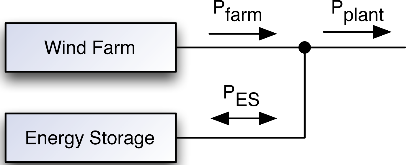
In the Pacific Northwest, utility reserve services are provided by generation from the Federal Columbia River Power System (FCRPS) (i.e., hydropower). The FCRPS is subject to a wide variety of constraints, including fish migration, flood control, recreation, river traffic control, and electrical power generation. The increase in variability from the growing wind power resource has begun to exhaust the reserve capacity of the system [2]. According to the Northwest Power and Conservation Council (NPCC), hydropower makes up 56% of online generating capacity in the Pacific Northwest as of February 2012, with wind accounting for 12% [3]. Most of the installed wind in the Pacific Northwest is in the Columbia River Gorge, a relatively small geographic area [4]. This means that when the wind rapidly increases, power generation from wind can go from nearly 0 MW to over 4000 MW in a matter of hours, meaning that several thousand megawatts of generation must be reduced somewhere else on the system in a short period of time. This reserve service is provided primarily by hydropower generation. The research presented in this paper investigates large-scale on-site energy storage as an alternative source of reserve capacity, as shown in Figure 2.

This paper will focus on simulations that combine a wind farm with a grid-scale energy storage source in the form of a zinc-bromine battery system. The addition of the energy storage source is meant to increase the dispatchability and reliability of the wind farm. A novel model predictive control (MPC) system has been developed for use with this combined system. Previous work has shown that energy storage can be used to increase wind power predictability and reduce variability in renewable energy plants [5–10]. In particular, Khatamianfar et al. [6] demonstrated an improvement in wind farm revenue of 3% when energy storage was added to the wind plant, and Teleke et al. [10] demonstrated that reducing the prediction horizon from 30 min to 15 min improved the performance of a wind and energy storage system by 14%. Additionally, many other control approaches have been tested and the results suggest that the combination of energy storage and wind power is technically and financially feasible [5,11–14].

There are few publications in the literature on the formulation and qualitative analysis of the performance of energy storage for wind farms, particularly utilizing MPC. Explorations of the effectiveness of the addition of energy storage with and without predictive control and different types of power scheduling and forecasting will be discussed.

2. Methodology

2.1. Proposed Control Structure

In this research, a MPC structure has been implemented. For MPC, current and future control actions are determined in the context of predicted plant behavior. At each sample time, the plant states are measured (or estimated) and any known plant disturbances are predicted over some length of time into the future (i.e., the prediction horizon). A time series of control actions are then determined to drive the plant to a desired trajectory over the prediction horizon. The first control action of the time series is applied to the plant and the process is repeated at the next sample time [15].

One of the benefits of having a predictive controller, as opposed to a reactive controller [16], is that the system can take preparatory actions to mitigate the negative effects of events such as wind ramps before they happen. Additionally, the MPC structure contains limit and cost information on both the plant and control actions.

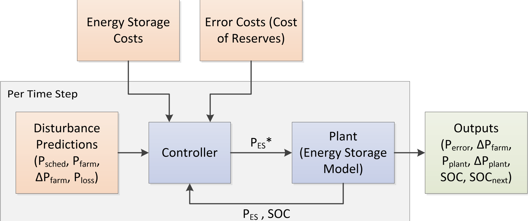
Figure 3 shows a block diagram of the model predictive controller including inputs, system control, and outputs. The controller takes the predicted wind data as inputs and produces an energy storage power command as output. Additional parameters include system limits and costs associated with control commands. The inputs and outputs for this research will be discussed further below.

2.2. Model Predictive Control Formulation

In this section, we formulate the discrete-time plant predictive model. In discrete time, the state update equation can be seen in Equation (1) and the output equation in Equation (2):

$$\mathbf{x}\left(k+1\right)=\mathbf{A}x\left(k\right)+{\mathbf{B}}_u\mathbf{u}\left(k\right)+{\mathbf{B}}_v\mathbf{v}\left(k\right)$$

(1)

$$\mathbf{y}\left(k\right)=\mathbf{C}x\left(k\right)+{\mathbf{D}}_u\mathbf{u}\left(k\right)+{\mathbf{D}}_v\mathbf{v}\left(k\right)$$

(2)

In Equation (1), x(k + 1) gives the system state one step in the future, A is the state matrix, x(k) is the current system state, B_u is the input control matrix, u(k) is the input control vector, B_v is the input disturbance matrix, and v(k) is the input disturbance vector. In Equation (2), y(k) is the output vector, C is the output matrix, D_u is the feedthrough input control matrix, and D_v is the feedthrough input disturbance matrix. To form the predictive model over the prediction horizon H_p, Equations (1) and (2) are incremented one sample into the future and recursively back-substituted, yielding the predictive model shown in Equations (3) and (4) [15]:

$$\begin{array}{cc}\hfill \underset{\overrightarrow{\mathbf{y}}(k)}{\underbrace{\left[\begin{array}{c}\mathbf{y}\left(k\right)\\ \mathbf{y}\left(k+1\right)\\ \mathbf{y}\left(k+2\right)\\ ⋮\\ \mathbf{y}\left(k+H_p\right)\end{array}\right]}}=\hfill & \hfill \underset{{\mathbf{S}}_x}{\underbrace{\left[\begin{array}{c}\mathbf{C}\\ \mathbf{C}\mathbf{A}\\ \mathbf{C}{\mathbf{A}}^2\\ ⋮\\ \mathbf{C}{\mathbf{A}}^{H_p}\end{array}\right]}}\mathbf{x}\left(k\right)+\underset{{\mathbf{S}}_u}{\underbrace{\left[\begin{array}{ccccc}\hfill {\mathbf{D}}_u\hfill & \hfill 0\hfill & \hfill 0\hfill & \hfill \dots \hfill & \hfill 0\hfill \\ \hfill \mathbf{C}{\mathbf{B}}_u\hfill & \hfill {\mathbf{D}}_u\hfill & \hfill 0\hfill & \hfill \dots \hfill & \hfill 0\hfill \\ \hfill \mathbf{C}\mathbf{A}{\mathbf{B}}_u\hfill & \hfill \mathbf{C}{\mathbf{B}}_u\hfill & \hfill {\mathbf{D}}_u\hfill & \hfill \dots \hfill & \hfill 0\hfill \\ \hfill ⋮\hfill & \hfill ⋮\hfill & \hfill ⋮\hfill & \hfill \ddots \hfill & \hfill ⋮\hfill \\ \hfill \mathbf{C}{\mathbf{A}}^{H_p-1}{\mathbf{B}}_u\hfill & \hfill \mathbf{C}{\mathbf{A}}^{H_p-2}{\mathbf{B}}_u\hfill & \hfill \dots \hfill & \hfill \mathbf{C}{\mathbf{B}}_u\hfill & \hfill {\mathbf{D}}_u\hfill \end{array}\right]}}\underset{\overrightarrow{\mathbf{u}}(k)}{\underbrace{\left[\begin{array}{c}\mathbf{u}\left(k\right)\\ \mathbf{u}\left(k+1\right)\\ \mathbf{u}\left(k+2\right)\\ ⋮\\ \mathbf{u}\left(k+H_p\right)\end{array}\right]}}\hfill \\ \hfill \hfill & \hfill +\underset{{\mathbf{S}}_v}{\underbrace{\left[\begin{array}{ccccc}\hfill {\mathbf{D}}_v\hfill & \hfill 0\hfill & \hfill 0\hfill & \hfill \dots \hfill & \hfill 0\hfill \\ \hfill \mathbf{C}{\mathbf{B}}_u\hfill & \hfill {\mathbf{D}}_v\hfill & \hfill 0\hfill & \hfill \dots \hfill & \hfill 0\hfill \\ \hfill \mathbf{C}\mathbf{A}{\mathbf{B}}_v\hfill & \hfill \mathbf{C}{\mathbf{B}}_v\hfill & \hfill {\mathbf{D}}_v\hfill & \hfill \dots \hfill & \hfill 0\hfill \\ \hfill ⋮\hfill & \hfill ⋮\hfill & \hfill ⋮\hfill & \hfill \ddots \hfill & \hfill ⋮\hfill \\ \hfill \mathbf{C}{\mathbf{A}}^{H_p-1}{\mathbf{B}}_v\hfill & \hfill \mathbf{C}{\mathbf{A}}^{H_p-2}{\mathbf{B}}_v\hfill & \hfill \dots \hfill & \hfill \mathbf{C}{\mathbf{B}}_v\hfill & \hfill {\mathbf{D}}_v\hfill \end{array}\right]}}\underset{\overrightarrow{\mathbf{v}}(k)}{\underbrace{\left[\begin{array}{c}\mathbf{v}\left(k\right)\\ \mathbf{v}\left(k+1\right)\\ \mathbf{v}\left(k+2\right)\\ ⋮\\ \mathbf{v}\left(k+H_p\right)\end{array}\right]}}\hfill \end{array}$$

(3)

$$\overrightarrow{\mathbf{y}}\left(k\right)={\mathbf{S}}_x\mathbf{x}\left(k\right)+{\mathbf{S}}_u\overrightarrow{\mathbf{u}}\left(k\right)+{\mathbf{S}}_v\overrightarrow{\mathbf{v}}\left(k\right)$$

(4)

Note that y⃗ (k) is the concatenated current and predicted output vector, u⃗ (k) is the control vector, and v⃗ (k) is the concatenated current and predicted disturbance vector. The dimensions are:

$$\begin{array}{c}\hfill \overrightarrow{\mathbf{y}}\in {\Re }^{n_y\cdot \left(H_p+1\right)\times 1}\hfill \\ \hfill \overrightarrow{\mathbf{u}}\in {\Re }^{n_u\cdot \left(H_p+1\right)\times 1}\hfill \\ \hfill \overrightarrow{\mathbf{v}}\in {\Re }^{n_v\cdot \left(H_p+1\right)\times 1}\hfill \\ \hfill {\mathbf{S}}_x\in {\Re }^{n_y\cdot \left(H_p+1\right)\times n_x}\hfill \\ \hfill {\mathbf{S}}_u\in {\Re }^{n_y\cdot \left(H_p+1\right)\times n_u\cdot \left(H_p+1\right)}\hfill \\ \hfill {\mathbf{S}}_v\in {\Re }^{n_y\cdot \left(H_p+1\right)\times n_v\cdot \left(H_p+1\right)}\hfill \end{array}$$

(5)

where n_x is the number of states; n_y is the number of outputs; n_u is the number of inputs; n_v is the number of disturbances; and H_p is the prediction horizon.

The quadratic tracking objective function is shown in Equation (6), where t⃗ (k) is the desired plant trajectory and is of the same dimension as Y⃗ (k:

$$J\left(k\right)={\left(\overrightarrow{\mathbf{t}}\left(k\right)-\overrightarrow{\mathbf{y}}\left(k\right)\right)}^T\hspace{0.17em}\mathbf{Q}\left(\overrightarrow{\mathbf{t}}\left(k\right)-\overrightarrow{\mathbf{y}}\left(k\right)\right)+\overrightarrow{\mathbf{u}}{\left(k\right)}^T\mathbf{R}\overrightarrow{\mathbf{u}}\left(k\right)$$

(6)

The matrices Q and R determine the costs associated with tracking errors and control actions, respectively. The dimensions are:

$$\begin{array}{c}\hfill \mathbf{Q}\in {\Re }^{n_y\cdot \left(H_p+1\right)\times n_y\cdot (H_p+1)}\hfill \\ \hfill \mathbf{R}\in {\Re }^{n_u\cdot \left(H_p+1\right)\times n_u\cdot (H_p+1)}\hfill \end{array}$$

(7)

Next, we manipulate Equation (6) such that u⃗ (k) is the only independent variable. A new variable e⃗ (k), the free evolution error, is defined in Equation (8). This is the resulting tracking error under the influence of only disturbance inputs and no control actions:

$$\begin{array}{cc}\hfill \overrightarrow{\mathbf{e}}(k)\hfill & \hfill =\overrightarrow{\mathbf{t}}(k)-\left(\overrightarrow{\mathbf{y}}(k)-{\mathbf{S}}_u\overrightarrow{\mathbf{u}}\left(k\right)\right)\hfill \\ \hfill \hfill & \hfill =\overrightarrow{\mathbf{t}}(k)-\left({\mathbf{S}}_x\mathbf{x}(k)+{\mathbf{S}}_v\overrightarrow{\mathbf{v}}\left(k\right)\right)\hfill \end{array}$$

(8)

Substituting Equation (8) into Equation (6) yields:

$$J\left(k\right)=\overrightarrow{\mathbf{u}}{\left(k\right)}^T\left({\mathbf{S}}_u^T\mathbf{Q}{\mathbf{S}}_u+\mathbf{R}\right)\overrightarrow{\mathbf{u}}\left(k\right)-2\overrightarrow{\mathbf{e}}{\left(k\right)}^T\mathbf{Q}{\mathbf{S}}_u\overrightarrow{\mathbf{u}}\left(k\right)+\overrightarrow{\mathbf{e}}{\left(k\right)}^T\mathbf{Q}\overrightarrow{\mathbf{e}}\left(k\right)$$

(9)

The bias terms are removed and the equation rescaled to yield the cost function for optimization:

$$\widehat{J}\left(k\right)=\widehat{J}\left(\overrightarrow{\mathbf{u}}\left(k\right)\right)=\frac{1}{2}\overrightarrow{\mathbf{u}}{\left(k\right)}^T\left({\mathbf{S}}_u^T\mathbf{Q}{\mathbf{S}}_u+\mathbf{R}\right)\overrightarrow{\mathbf{u}}\left(k\right)-\overrightarrow{\mathbf{e}}{\left(k\right)}^T\mathbf{Q}{\mathbf{S}}_u\overrightarrow{\mathbf{u}}\left(k\right)$$

(10)

Equation (10) represents a quadratic programming problem in which the vector u⃗ (k) is determined to minimize Ĵ(k) in the context of constraints on u⃗ (k).

For MPC implementation, the current control action u(k) is taken from the predicted control vector u⃗ (k) and applied to the plant. At the next time step, Equation (8) is recalculated and the quadratic programming problem of Equation (10) is resolved, a new u(k) is determined, and the process repeats for each subsequent time sample.

2.3. Model Predictive Control Implementation

In this application, a large-scale energy storage system is collocated with a wind farm such that the on-site energy storage provides reserves for the wind generation. The energy storage power output is controlled in such a way that the combined wind farm and energy storage output can match the scheduled wind power output. The plant model is given in Equations (11) and (12):

$$\begin{array}{cccc}\underset{\mathbf{x}\left(k+1\right)}{\underbrace{{\left[\begin{array}{c}\mathit{SOC}\\ P_{\text{ES},\text{prev}}\end{array}\right]}_{k+1}}}& =\underset{\mathbf{A}}{\underbrace{\left[\begin{array}{cc}1& 0\\ 0& 0\end{array}\right]}}\underset{\mathbf{x}\left(k\right)}{\underbrace{{\left[\begin{array}{c}\mathit{SOC}\\ P_{\text{ES},\text{prev}}\end{array}\right]}_k}}& +\underset{{\mathbf{B}}_u}{\underbrace{\left[\begin{array}{c}-m_{\Delta }\\ 1\end{array}\right]}}\underset{\mathbf{u}\left(k\right)}{\underbrace{{\left[P_{\text{ES}}\right]}_k}}& +\underset{{\mathbf{B}}_u}{\underbrace{\left[\begin{array}{cccc}0& 0& 0& -m_{\Delta }\\ 0& 0& 0& 0\end{array}\right]}}\end{array}\underset{\text{v}\left(k\right)}{\underbrace{{\left[\begin{array}{c}{P}_{\text{sched}}\\ P_{\text{farm}}\\ \Delta P_{\text{farm}}\\ P_{\text{loss}}\end{array}\right]}_k}}$$

(11)

$$\begin{array}{cccc}\underset{\mathbf{y}\left(k\right)}{\underbrace{{\left[\begin{array}{c}\hfill P_{\text{err}}\hfill \\ \hfill \mathrm{\Delta }{P}_{\text{ES}}\hfill \\ \hfill P_{\text{plant}}\hfill \\ \hfill \mathrm{\Delta }{P}_{\text{plant}}\hfill \\ \hfill \mathit{SOC}\hfill \\ \hfill {\mathit{SOC}}_{\text{next}}\hfill \end{array}\right]}_k}}& =\underset{\mathbf{C}}{\underbrace{\left[\begin{array}{cc}0& 0\\ 0& -1\\ 0& 0\\ 0& -1\\ 1& 0\\ 1& 0\end{array}\right]}}\underset{\mathbf{x}\left(k\right)}{\underbrace{{\left[\begin{array}{c}\mathit{SOC}\\ P_{\text{ES},\text{prev}}\end{array}\right]}_k}}& +\underset{{\mathbf{D}}_u}{\underbrace{\left[\begin{array}{c}-1\\ 1\\ 1\\ 1\\ 0\\ -m_{\mathrm{\Delta }}\end{array}\right]}}\underset{\mathbf{u}\left(k\right)}{\underbrace{{\left[P_{\text{ES}}\right]}_k}}& +\underset{{\mathbf{D}}_u}{\underbrace{\left[\begin{array}{cccc}1& -1& 0& 0\\ 0& 0& 0& 0\\ 0& 1& 0& 0\\ 0& 0& 1& 0\\ 0& 0& 0& 0\\ 0& 0& 0& -m_{\mathrm{\Delta }}\end{array}\right]}}\end{array}\underset{\mathbf{v}\left(k\right)}{\underbrace{{\left[\begin{array}{c}{P}_{\text{sched}}\\ P_{\text{farm}}\\ \mathrm{\Delta }{P}_{\text{farm}}\\ P_{\text{loss}}\end{array}\right]}_k}}$$

(12)

In Equation (11), SOC is the state of charge of the energy storage source, SOC_next is the next SOC based on the losses and current energy storage command, P_ES,prev is the energy storage command from the last time step, m_Δ is the per-unit per-sample capacity constant of the energy storage source, P_ES is the current energy storage command, P_sched is the scheduled output of the wind farm, P_farm is the actual output of the wind farm, and P_loss is the approximate loss in the energy storage source. In Equation (12)P_err = P_sched − P_plant, where P_plant is the combined wind farm and energy storage output. The loss is included in the control model as an independent disturbance term to maintain linearity. It is positive for both positive and negative values of P_ES, and for predictive purposes can be set as a constant to include both the self-discharge rate and an approximation of the power-dependent losses under normal usage.

In this research, the sample time of the discrete model shown above is 10 min. The dynamic response of a zinc-bromine battery system is generally much faster than 10 min (it is expected to be in the order of seconds). Therefore, the dynamic response of the system is not included in the model in Equations (11) and (12). In other words, the commanded energy storage power output is assumed to always be equal to the actual power output.

The objective function weighting is shown in Equations (13)–(15). The individual terms in q are the corresponding weights for the entries of the output vector y(k). The dimension of Q is n_y · (H_p + 1) × n_y · (H_p + 1), and the dimension of R is n_u · (H_p + 1) × n_u · (H_p + 1). In this research, the matrices Q and R are purely diagonal as there is no need to weight cross-coupling terms or have the weights vary across the prediction horizon:

$$\mathbf{q}=\left[\begin{array}{cccccc}{q}_{P_{\text{err}}}& 0& 0& 0& 0& 0\\ 0& q_{\Delta P_{\text{ES}}}& 0& 0& 0& 0\\ 0& 0& q_{P_{\text{plant}}}& 0& 0& 0\\ 0& 0& 0& q_{\Delta P_{\text{plant}}}& 0& 0\\ 0& 0& 0& 0& q_{\mathit{SOC}}& 0\\ 0& 0& 0& 0& 0& q_{{\mathit{SOC}}_{\text{next}}}\end{array}\right]$$

(13)

$$\mathbf{Q}=\left[\begin{array}{ccc}{\mathbf{q}}_k& \mathbf{0}& \mathbf{0}\\ \mathbf{0}& \mathbf{\ddots }& \mathbf{0}\\ \mathbf{0}& \mathbf{0}& {\mathbf{q}}_{k+H_p}\end{array}\right]$$

(14)

$$\mathbf{R}=\left[\begin{array}{ccc}{\left[r_{P_{\text{ES}}}\right]}_k& \mathbf{0}& \mathbf{0}\\ \mathbf{0}& \ddots & \mathbf{0}\\ \mathbf{0}& \mathbf{0}& {\left[r_{P_{\text{ES}}}\right]}_{k+H_p}\end{array}\right]$$

(15)

Constraints for this implementation are shown in Equations (16) and (17):

$$\left[\begin{array}{c}{P}_{\text{ES}}\\ -P_{\text{ES}}\end{array}\right]\le \left[\begin{array}{c}{P}_{\text{ES},\text{upper}}\\ P_{\text{ES},\text{lower}}\end{array}\right]$$

(16)

$$\left[\begin{array}{c}\mathit{SOC}\\ -\mathit{SOC}\\ {\mathit{SOC}}_{\text{next}}\\ -{\mathit{SOC}}_{\text{next}}\end{array}\right]\le \left[\begin{array}{c}{\mathit{SOC}}_{\text{upper}}\\ -{\mathit{SOC}}_{\text{lower}}\\ {\mathit{SOC}}_{\text{upper}}\\ -{\mathit{SOC}}_{\text{lower}}\end{array}\right]$$

(17)

3. Simulation Results

3.1. Simulation Setup

For the simulations, a large-scale energy storage system is collocated with a wind farm such that the on-site energy storage provides reserves for the wind generation. The wind farm nameplate capacity is 100 MW and the energy storage system is rated for 25 MW (power) and 50 MW·h (energy); this sizing, relative to the wind farm capacity, is based on considerations of existing large-scale energy storage systems, hardware availability, and sizing analysis from literature [17].

Wind farm power forecast and actual data were obtained from the Bonneville Power Administration (BPA) as matched historical data [18] (i.e., for every time index, the wind farm power is matched with forecasted wind farm power from that index onward). Simulations were conducted with data from the week of 26 March 2012 to 1 April 2012, comprised of 888 10-min samples. When the simulations were conducted, actual power data and forecasted wind power output for all wind on the BPA system were available as an aggregate, not for individual wind farms. The presented research assumes that the energy storage system to be simulated is for a single wind farm. Thus, the aggregate power and forecast data was scaled and used to represent a single farm. The aggregate data includes smoothing due to geographic diversity, which would not be present in data from an individual wind farm. Utilizing individual wind farm data will improve simulation accuracy when high-resolution data becomes available. The forecasted wind power was provided by a third-party meteorological forecasting firm (an example is presented in the Appendix). The wind farm scheduled output, P_sched, is determined by a persistence method. Both 60 min and 30 min scheduling intervals were used.

The primary control objective is to utilize the energy storage system to minimize P_err, which is the difference between the scheduled wind farm output (P_sched) and the combined wind farm and energy storage output (P_plant = P_farm + P_ES). Plant ramp rates (i.e., ΔP_plant) can also be considered within the control objective as well.

The predicted disturbance vector, v⃗ (k), requires predictions of both the wind farm scheduled output (P_sched(k|k), P_sched(k + 1|k), ⋯, P_sched(k + H_p|k)) and the wind farm actual output (P_farm(k|k), P_farm(k +1|k), ⋯, P_farm(k +H_p|k)) over the prediction horizon, H_p. Both of these predictions are based on the meteorological forecast at time k.

The cost q_Perr in Q, which is the cost of the mismatch between scheduled and actual plant output over the sample time, was determined from the BPA variable energy resource balancing service (VERBS) rate, which is currently charged to wind farms monthly based on installed capacity. The VERBS charge is currently 1.23 $/kW/mo of capacity and can be subdivided into regulating reserves for balancing moment to moment (0.08 $/kW/mo), following reserves for balancing larger mismatches within the hour (0.37 $/kW/mo), and imbalance reserves for balancing the difference between the generators schedule and the actual generation during 1 h (0.78 $/kW/mo) [19].

In order to translate VERBS into a real-time cost, scheduling error was summed over four months for a 100 MW wind farm in the Pacific Northwest. This error was then divided by the cost for four months of the VERBS service. The result is the constant q_Perr in the unit of $/PU². Initially, this study explores the effectiveness of a model predictive controller to reduce error and/or ramp rate, and thus initially sets r_PES in R to zero, which is the cost of the energy storage output over the sample time. Future work will focus on including this cost in the analysis, which is explicitly one of the strengths of the MPC approach outlined here.

Losses were included in the model as a constant power loss and modeled after the chemical leakage losses of the zinc-bromine battery in the Wallace Energy Systems and Renewables Facility (WESRF) lab. Approximately 1% of the total energy capacity is lost each hour, except at SOC levels below 2% where losses become extremely low.

Controller constraints are specified for energy storage power and state of charge. The energy storage power constraints, P_ES,upper and P_ES,lower, are set to 0.25 PU and −0.25 PU, respectively, based on the limits of the zinc-bromine battery available in the WESRF lab. The state of charge constraints, SOC_upper and SOC_lower, were set to 1 PU and 0 PU representing the safe full and empty states of charge, respectively. Simulations were performed with a 10 min sample time. The capacity of the energy storage system is 0.50 PUhr and therefore the per-unit per-sample capacity constant in Equation (11) is $m_{\Delta }=(0.50\hspace{0.17em}\hspace{0.17em}\hspace{0.17em}\mathit{PU}hr)\cdot \left(\frac{1}{6}\hspace{0.17em}\hspace{0.17em}\hspace{0.17em}hr/\text{sample}\right)/(0.25\hspace{0.17em}\hspace{0.17em}\hspace{0.17em}\mathit{PU})=1/3$. Each simulation covers a week.

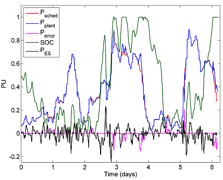
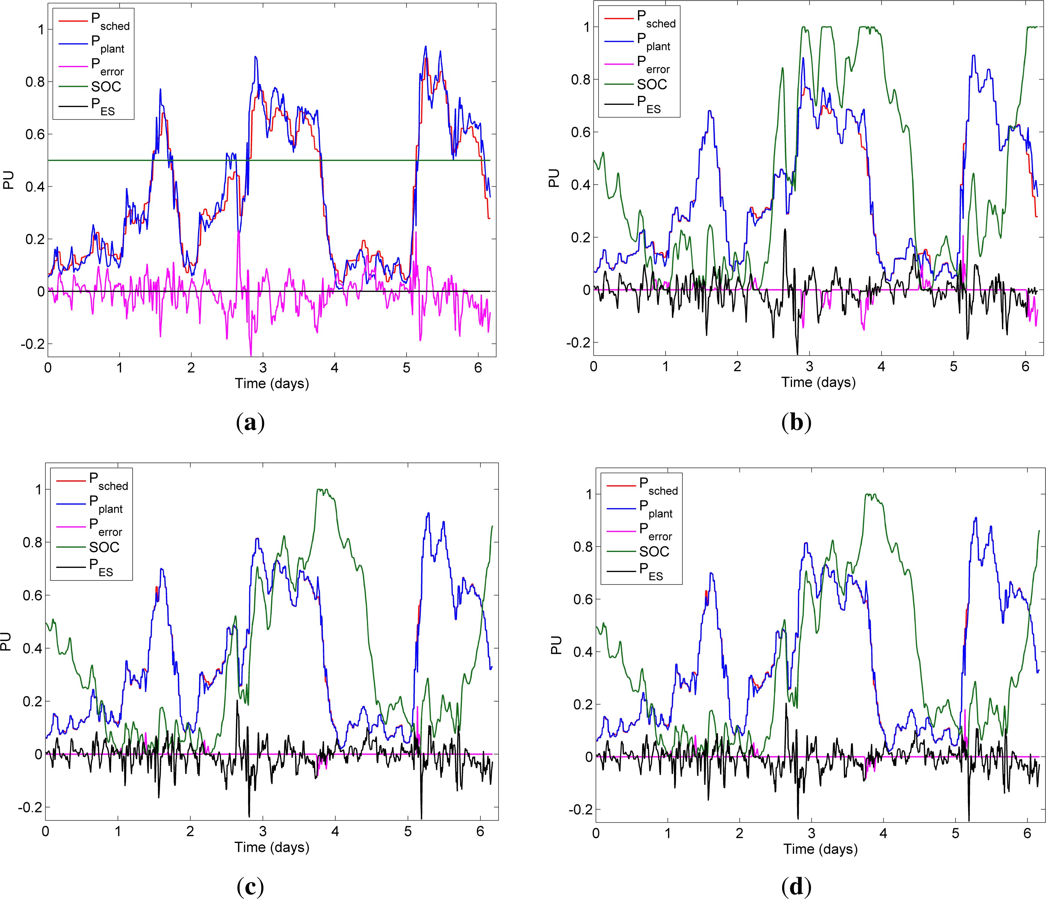
In order to explore the effectiveness of MPC on minimizing P_err, five cases were examined. Figure 4(a) shows Case 1 with no energy storage or MPC. Figure 4(b)–4(d) shows the effects of enabling the use of energy storage, enabling predictive control, and shortening scheduling length from 60 min to 30 min, respectively (Cases 2, 3, and 5). The figures demonstrate that error can be reduced by adding energy storage and even further by reducing scheduling length from 60 min to 30 min.

The addition of MPC, as opposed to simple reactive control, also makes a significant difference but is better observed quantitatively in

Table 1. Simulation results over approximately one week (888 10-min samples). Percent change from the base case, Case 1, is shown in parenthesis. MAE: mean absolute error.

Case	1	2	3	4	5
Scheduling interval	60 min	60 min	60 min	30 min	30 min
Energy storage	Inactive	Active	Active	Active	Active
Predictive control	NA	Off	On	Off	On
Perr MAE	0.0454	0.0086 (−81)	0.0088 (−81)	0.0021 (−95)	0.0022 (−95)
JQ,err ($)	8211	1670 (−80)	1546 (−81)	346 (−96)	275 (−97)
Following reserve (PU)	0.2338	0.1467 (−37)	0.1039 (−56)	0.0937 (−60)	0.0573 (−75)
Imbalance reserve (PU)	0.3221	0.2375 (−26)	0.2290 (−29)	0.1335 (−59)	0.1272 (−61)

.

Table 1 shows the results corresponding to the five cases. Four different metrics were examined: mean absolute error (MAE) for the P_err time series, the error cost, and the following and imbalance reserve requirements. The error cost is defined below. In this analysis, N equals 888, which is the number of 10-min time steps used from the week of 26 March 2012:

$$J_{\text{Q},\text{err}}=\sum _i^N{q}_{P_{\text{err}}}{P}_{\text{err}}{\left(i\right)}^2\hspace{0.17em}\hspace{0.17em}\hspace{0.17em}\hspace{0.17em}(\$)$$

(18)

Following reserves are calculated by taking the difference between hourly average power and 10 min power, whereas imbalance reserves are the difference between the scheduled hourly power and the hourly average power actually produced. The reserve metrics in the table represent the sum of the incremental (inc) and decremental (dec) reserves, which gives the amount of additional generation that must be available to either increase (inc) or decrease (dec) to balance wind fluctuations [20,21].

Case 1 in Table 1 presents the metrics for the base case, with no energy storage sources active. Case 2 presents the results with energy storage enabled and with predictive control off. In the cases without predictive control, the prediction horizon is effectively set to zero, such that the control command only corrects the error at the current time step (with no optimization of future time steps). Comparing the metrics in these two cases, it is clear that the addition of energy storage can significantly reduce error and improve reserve requirements (e.g., reducing the following reserve by 37%).

Case 3 in Table 1 presents the results with predictive control enabled. Based on empirical analysis, a prediction horizon (H_p) of 2 h was chosen for the predictive control cases. Comparing Case 3 with Case 2, it is clear that, while predictive control does not have a major impact on the error—merely a very slight improvement in J_Q,err—there is an improvement in reserves. This is because J_Q,err is a weighted sum of all quadratic errors and is thus not generally dominated by any single sample. The reserve calculation on the other hand is largely determined by outlier events. For example, the single largest deviation within the hour with respect to the average over the entire year dictates the value of following reserve. Therefore we can see that the primary value of the predictive element is an improvement in the boundary (i.e., outlier) cases. The strength of the predictive controller becomes more apparent when the number of optimization objectives and constraints increases (as presented in the following sections). Case 4 is provided for completeness to show the results for a scheduling interval of 30 min with predictive control off (figure not shown). Case 5 presents the results for a scheduling interval of 30 min with predictive control on. Finally, a comparison of Cases 3 and 5 shows the benefit of the scheduling horizon reduction, for which there is approximately a four-fold reduction in the P_err MAE. Therefore, we can see that the scheduling horizon is a very significant factor. The trend in the utility industry in the US is to shorten scheduling times. This effectively shifts the burden of variability from reserve generation to scheduled generation, so this may be a larger factor in reducing reserve requirements for wind farms than energy storage technology in the future.

3.2. Minimizing ΔP_plant

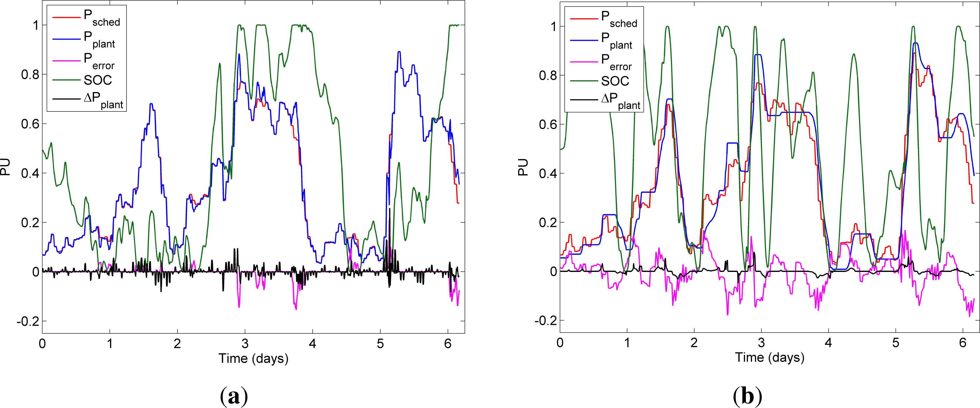
In order to examine the predictive controller’s ability to minimize wind ramps, the cost of plant ramps, q_ΔPplant, was set to a non-zero value. This enabled the controller to minimize ramp events by considering the cost of those events in the control action. A ramp was defined as a 0.20 PU change in plant output over 1 h. This is based on the BPA definition of persistent deviation found in [19]. Figure 5(a),5(b) can be compared to see the difference between error reduction and ramp reduction; Cases 3 and 6, respectively. The black trace in each figure shows the ΔP_plant time series. It is clear that in the error reduction case (Figure 5(a)), ΔP_plant is uncontrolled, while in the ramp reduction case (Figure 5(b)), ΔP_plant is minimized (at the expense of P_err). The P_plant time series in Figure 5(b) has much slower gradual changes over time compared with Figure 5(a).

Quantitative results for ramp reduction are shown in

Table 2. Summary of error reduction, ramp reduction, and combined optimization cases over approximately one week (888 10-min samples). Percent change from the base case, Case 1, is given in parenthesis. Comparing Cases 7 and 8 with Case 3, it is shown that ramp events can be reduced with only a minimal impact on scheduling error. Compared with the base case, Case 1, it is shown that the scheduling error and the number of ramp events can be simultaneously improved.

Case	1	3	6	7	8
Objective	Base case	Error reduction	Ramp reduction	Combined optimization
Energy storage	Inactive	Active	Active	Active	Active
Error cost (qPerrs)	2503	2503	0	2503	2503
Ramp cost (qΔPplant)	0	0	600	600	6000
Perr MAE	0.0454	0.0088 (−81)	0.0515 (+13)	0.0101 (−78)	0.0141 (−69)
JQ,err ($)	8211	1546 (−81)	0	1563 (−81)	1859 (−77)
JQ,ramp ($)	0	0	68	183	1133
JQ,err + JQ,ramp ($)	8211	1546 (−81)	68 (−99)	1746 (−79)	2992 (−64)
Ramps up	53	45 (−15)	14 (−74)	32 (−40)	16 (−70)
Ramps down	55	39 (−29)	1 (−98)	30 (−45)	12 (−78)
Total ramps	108	84 (−22)	15 (−86)	62 (−43)	28 (−74)

.

3.3. Minimizing P_err and ΔP_plant (Combined)

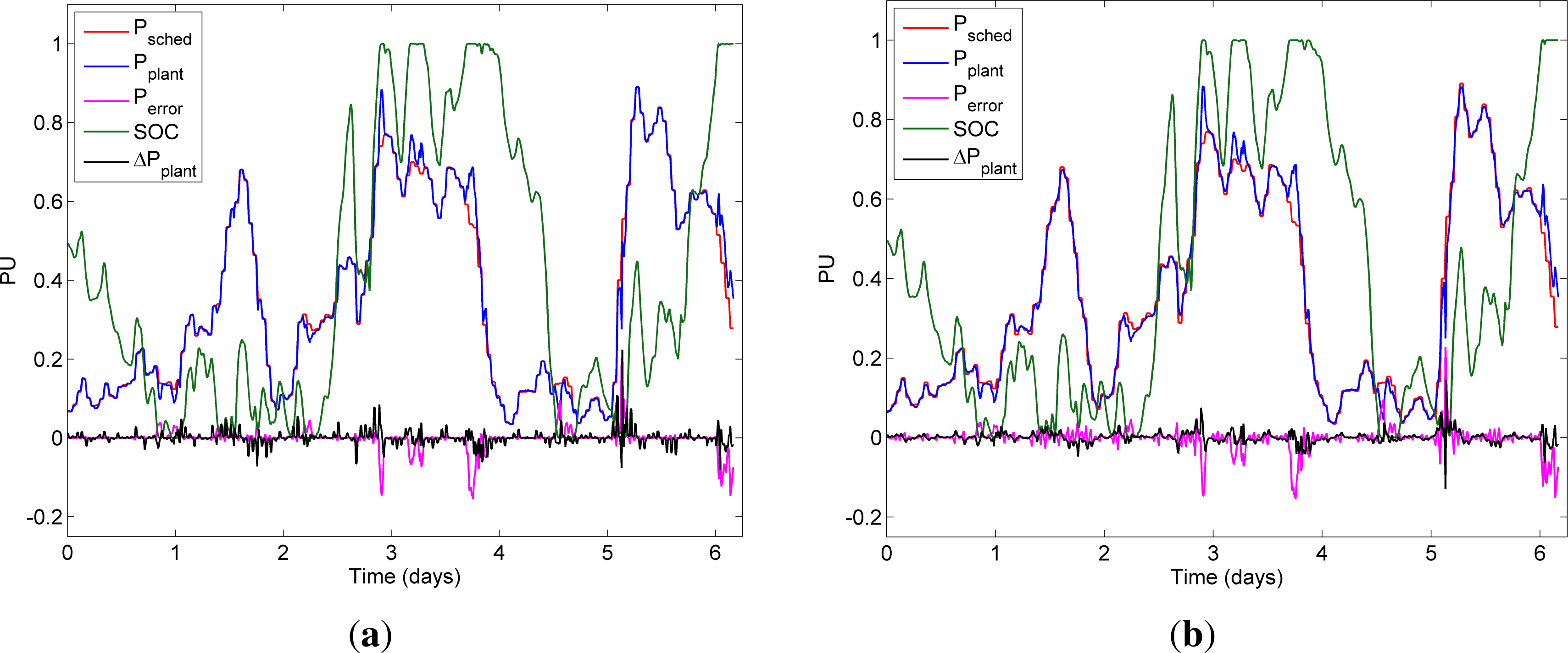
The strength of the MPC approach is best demonstrated when multiple objectives and constraints are simultaneously considered: minimizing error while also minimizing ramps. This scenario is significant because it shows that the addition of energy storage with proper control can reduce both error and ramping, which lessens the need for balancing from reserves. Figure 6(a),6(b) demonstrates two different combined optimization cases (Cases 7 and 8) where both error and wind ramps were simultaneously minimized by the controller. In Case 7, the ramp cost is 600 $/PU² and in Case 8 the ramp cost is 6000 $/PU². The ramp costs for these cases were selected by sweeping the cost over a wide range and examining the resulting output parameters to experimentally determine appropriate values for presentation.

Similar to Table 1, various metrics are presented in order to quantify the performance of the controller. In addition to MAE of P_err, the table shows a breakdown of the cumulative error (J_Q,err) and cumulative ramp (J_Q,ramp) costs, as well as the total cost for each case. Equation (18) is the cumulative error cost, and the cumulative ramp cost is defined in Equation (19):

$$J_{\text{Q},\text{ramp}}=\sum _i^N{q}_{\Delta P_{\text{plant}}}\Delta P_{\text{plant}}{\left(i\right)}^2\hspace{0.17em}\hspace{0.17em}\hspace{0.17em}\hspace{0.17em}\hspace{0.17em}\hspace{0.17em}\hspace{0.17em}(\$)$$

(19)

The last three rows of the table present a count of the number of up, down, and total ramps, where a ramp is defined as a 0.20 PU change (or greater) over 1 h, and the ramp count is determined through a sliding window over the P_plant time series.

In Table 2, Cases 1 and 3 are presented again as before, and Cases 6, 7 and 8, which address ramping, are presented as well. It is clear that with only a minimal increase in the overall error (from an MAE of 0.0088 to an MAE of 0.0141), the number of ramp events can be significantly decreased from 84 in Case 3 (error reduction only) to 28 in Case 8 (combined error and ramp reduction).

4. Conclusions

This paper presents an analysis of energy storage and MPC for improving the dispatchability of a large-scale wind farm. It has been shown that large-scale energy storage can be utilized to provide on-site balancing reserves for a wind farm. Energy storage with predictive control can reduce the scheduling error by approximately 80% and decrease the following reserve and the imbalance reserve by approximately 35% and 25%, respectively (compared with a base case of no on-site energy storage).

One of the significant advantages of MPC is the ability to simultaneously consider several objectives in the context of system constraints. This has also been demonstrated by a reduction in scheduling error of approximately 70% and a simultaneous reduction in ramp events of approximately 75%, when both aspects are weighted in the cost function. Increasing the weight on ramping will reduce ramping but cause more scheduling error. Increasing the weight on scheduling error will reduce scheduling error but cause more ramping.

It is also demonstrated that the scheduling horizon has a very significant impact on the scheduling error and the reserve requirements. Decreasing the scheduling horizon from 60 min to 30 min improves the scheduling error by an approximately additional 15% and improves the reserve requirements by an approximately additional 20% or more. Since the scheduling horizon is decided upon by the balancing area authority, it is not a degree of freedom for the energy storage system designer, but it is an important constraint that has a large impact on the system performance. Shorter scheduling horizons shift the burden of variability away from reserves to scheduled generation, thus possibly reducing the need for on-site energy storage for wind farms.

Overall, the research shows that MPC is very well suited for energy storage control of providing reserves for variable, renewable power generation.

References

- Wind Generation Capacity, 2012. Available online: http://transmission.bpa.gov/business/operations/Wind/WIND_InstalledCapacity_PLOT.pdf (accessed on 1 June 2013).
- Connecting Variable Generating Resources to the Federal Columbia River Transmission System (FCRTS); Bonneville Power Administration (BPA): Portland, OR, USA, 2010.
- Dragoon, K.; Charles, G. Historical Energy Production, Northwest Power and Conservation Council (NPCC), Portland, OR, USA, 2012.
- Current and Proposed Wind Project Interconnections to BPA Transmission Facilities; Bonneville Power Administration (BPA): Portland, OR, USA, 2011.
- Han, H.; Brekken, T.K.A.; von Jouanne, A.; Bistrika, A.; Yokochi, A. In-lab research grid for optimization and control of wind and energy storage systems. In Proceedings of the 2010 49th IEEE Conference on Decision and Control (CDC), Atlanta, GA, USA, 15–17 December 2010; pp. 200–205.
- Khatamianfar, A.; Khalid, M.; Savkin, A.; Agelidis, V. Improving wind farm dispatch in the Australian electricity market with battery energy storage using model predictive control. IEEE Trans. Sustain. Energy 2013, 4, 745–755. [Google Scholar]
- Perez, E.; Beltran, H.; Aparicio, N.; Rodriguez, P. Predictive power control for PV plants with energy storage. IEEE Trans. Sustain. Energy 2013, 4, 482–490. [Google Scholar]
- Qi, W.; Liu, J.; Christofides, P. Supervisory predictive control for long-term scheduling of an integrated wind/solar energy generation and water desalination system. IEEE Trans. Control Syst. Technol 2012, 20, 504–512. [Google Scholar]
- Thatte, A.; Zhang, F.; Xie, L. Coordination of wind farms and flywheels for energy balancing and frequency regulation. In Proceedings of the 2011 IEEE Power and Energy Society General Meeting, San Diego, CA, USA, 24–29 July 2011; pp. 1–7.
- Teleke, S.; Baran, M.E.; Bhattacharya, S.; Huang, A.Q. Optimal control of battery energy storage for wind farm dispatching. IEEE Trans. Energy Convers 2010, 25, 787–794. [Google Scholar]
- Baone, C.; DeMarco, C. Saturation-bandwidth tradeoffs in grid frequency regulation for wind generation with energy storage. In Proceedings of the 2011 IEEE PES Innovative Smart Grid Technologies (ISGT), Hilton Anaheim, CA, USA, 17–19 January 2011; pp. 1–7.
- Mendis, N.; Muttaqi, K.; Sayeef, S.; Perera, S. Control coordination of a wind turbine generator and a battery storage unit in a remote area power aupply system. In Proceedings of the 2010 IEEE Power and Energy Society General Meeting, Minneapolis, MN, USA, 25–29 July 2010; pp. 1–7.
- Banham-Hall, D.D.; Taylor, G.A.; Smith, C.A.; Irving, M.R. Frequency control using vanadium redox flow batteries on wind farms. In Proceedings of the 2011 IEEE Power and Energy Society General Meeting, San Diego, CA, USA, 24–29 July 2011; pp. 1–8.
- Fazeli, M.; Asher, G.; Klumpner, C.; Yao, L.; Bazargan, M.; Parashar, M. Novel control scheme for wind generation with energy storage supplying a given demand power. In Proceedings of the 2010 14th Power Electronics and Motion Control Conference (EPE/PEMC), Ohrid, Republic of Macedonia, 6–8 September 2010; pp. S14-15–S14-21.
- Rossiter, J. Model-based Predictive Control: A Practical Approach; CRC Press: Boca Raton, FL, USA, 2003. [Google Scholar]
- Antonishen, M.; Han, H.; Brekken, T.; von Jouanne, A.; Yokochi, A.; Halamay, D.; Song, J.; Naviaux, D.; Davidson, J.; Bistrika, A. A methodology to enable wind farm participation in automatic generation control using energy storage devices. In Proceedings of the 2012 IEEE Power and Energy Society General Meeting, San Diego, CA, USA, 22–26 July 2012; pp. 1–7.
- Brekken, T.K.A.; Yokochi, A.; von Jouanne, A.; Yen, Z.; Hapke, H.; Halamay, D. Optimal energy storage sizing and control for wind power applications. IEEE Trans. Sustain. Energy 2011, 2, 69–77. [Google Scholar]
- BPA Wind Generation in the Last 7 Days, 2012. Available online: http://transmission.bpa.gov/Business/Operations/Wind/baltwg.aspx (accessed on 1 June 2013).
- 2012 BPA Final Rate Proposal, Generation Inputs Study; Bonneville Power Administration (BPA): Portland, OR, USA, 2011.
- Reserve Capacity Forecast for Wind Generation within-hour Balancing Service; Bonneville Power Administration (BPA): Portland, OR, USA, 2008.
- Balancing and Frequency Control; North American Electric Reliability Corporation (NERC): Atlanta, GA, USA, 2011.