Towards a Friendly Energy Management Strategy for Hybrid Electric Vehicles with Respect to Pollution, Battery and Drivability

Abstract

The paper proposes a generic methodology to incorporate constraints (pollutant emission, battery health, drivability) into on-line energy management strategies (EMSs) for hybrid electric vehicles (HEVs) and plug-in hybrid electric vehicles (PHEVs). The integration of each constraint into the EMS, made with the Pontryagin maximum principle, shows a tradeoff between the fuel consumption and the constraint introduced. As state dynamics come into play (catalyst temperature, battery cell temperature, etc.), the optimization problem becomes more complex. Simulation results are presented to highlight the contribution of this generic strategy, including constraints compared to the standard approach. These results show that it is possible to find an energy management strategy that takes into account an increasing number of constraints (drivability, pollution, aging, environment, etc.). However, taking these constraints into account increases fuel consumption (the existence of a trade-off curve). This trade-off can be sometimes difficult to find, and the tools developed in this paper should help to find an acceptable solution quickly.

1. Introduction

The hybrid vehicle is one of the possible solutions for reducing greenhouse gas emissions in individual passenger transportation. Its ability to use various prime movers to satisfy the power demand allows the supervisory control to choose the energy flow that minimizes global greenhouse gas emissions, such as CO₂ emissions. In a hybrid electric vehicle, the torque split (the ratio between electrical and thermal torque) makes it possible to minimize fuel consumption and, hence, CO₂ emissions over the whole driving cycle. Most of the time, energy optimization in hybrid vehicles consists in minimizing the fuel consumption [1,2]:

$$J={\int }_{t_0}^{t_f}{\dot{m}}_f(\mathbf{u}(t),t)dt$$

(1)

where ṁ_f (u(t), t) is the instantaneous fuel consumption and u is the control vector, such as the electrical/thermal ratio. In a general manner, it can be written:

$$J={\int }_{t_0}^{t_f}L(\mathbf{u}(t),t)dt$$

(2)

where L(u(t), t) is the instantaneous cost function. The solution that minimizes Equation (2) is an electrical mode, in which the energy comes directly from the battery, which makes it impossible to maintain the battery state of charge x. Hence, the cost function must integrate a final constraint:

$$J=\mathrm{\Phi }\left(x(t_f)\right)+{\int }_{t_0}^{t_f}L(\mathbf{u}(t),t)dt$$

(3)

where Φ(x(t_f)) is a penalty function, which can be chosen to maintain the state of charge x(t_f) = x(t₀) [2,3]. Moreover, since the battery state of charge x is directly impacted by the chosen control, it is necessary to respect its dynamics: ẋ = f(x, u)

It is possible to add constraints to the energy management strategy, such as pollutant emission [4,5], engine events [6] or gear events [6,7], and this is what we will show in this paper. The first section recalls the classical optimal energy management strategy with the Pontryagin maximum principle. The second section shows how constraints can be easily incorporated into energy management strategies.

2. Optimal Energy Management Strategies

Energy management is a problem of optimal control with a finite horizon subject to system dynamics and final constraints. Let X ⊆ ℝⁿ and U ⊆ ℝ^m be the state and control sets. The m control variables are denoted u ∈ U and the n states denoted x ∈ X. The optimal control problem consists in minimizing J(x, u) ∈ ℝ with the following system dynamics:

$$\dot{\mathbf{x}}=f(\mathbf{x},\mathbf{u})$$

(4)

where (x, u) ↦ f(x, u) is a function of class $𝒞$¹. Moreover, an initial condition is imposed x(t₀) = x₀.

Hence, the optimization problem can be summarized in:

$$P_0(\mathbf{x},\mathbf{u}):\{\begin{array}{ll}\underset{\mathbf{u}\in U}{\text{min}}J(\mathbf{x},\mathbf{u})\hfill & \hfill \\ \text{subject}\hspace{0.17em}\text{to}\hfill & \dot{\mathbf{x}}=f(\mathbf{x},\mathbf{u})\hfill \\ \hfill & \mathbf{x}(t_0)={\mathbf{x}}_0\hfill \end{array}$$

(5)

with a performance index to minimize:

$$J(\mathbf{x},\mathbf{u})=\mathrm{\Phi }\left(\mathbf{x}(t_f)\right)+{\int }_{t_0}^{t_f}L\left(\mathbf{x}(t),\mathbf{u}(t),t\right)dt$$

(6)

where x ↦ Φ(x(t)) and (x, u, t) ↦ L(x, u, t) are of class $𝒞$¹.

In order to solve this problem, it is necessary to know the whole trip. As the driving conditions are generally not known in advance, the theoretical optimal solution of Problem (5) gives the achievable reference. Two methods have been developed to solve Problem (5), one numerical solution called dynamic programming [8–10] and one analytical solution called the equivalent dual problem [3,10]. The second solution, which is very interesting for real-time use in a vehicle, is presented here. It consists in defining a dual problem that has the same solution as the first one, while putting the constraints and the cost function into a single function.

Let us define the Hamiltonian:

$$H\left(\mathbf{x}(t),\mathbf{u}(t),\mathit{\lambda }(t),t\right)=L\left(\mathbf{x}(t),\mathbf{u}(t),t\right)+\mathit{\lambda }{(t)}^{T}f(\mathbf{x},\mathbf{u})$$

(7)

where λ is the Lagrange variable (or co-state) associated with the state x.

By grouping the three stationary conditions $\frac{\partial }{\partial \mathbf{x}}$, $\frac{\partial }{\partial \mathbf{u}}$, $\frac{\partial }{\partial \mathit{\lambda }}$, the dual problem P′₀(x, u) corresponding to P₀(x, u) is:

$$P_0^{\text{'}}(\mathbf{x},\mathbf{u})\{\begin{array}{l}\dot{\mathbf{x}}=f(\mathbf{x},\mathbf{u})\\ \mathbf{x}(t_0)={\mathbf{x}}^0\\ {\dot{\mathit{\lambda }}}^T=-\frac{\partial }{\partial \mathbf{x}}H(\mathbf{x},\mathbf{u},\mathit{\lambda },t)\\ \mathit{\lambda }{(t_f)}^T=\frac{\partial }{\partial \mathbf{x}(t_f)}\mathrm{\Phi }\left(\mathbf{x}(t_f)\right)\\ \text{where}\hspace{0.17em}\mathbf{u}\hspace{0.17em}\text{is}\hspace{0.17em}\text{the}\hspace{0.17em}\text{solution}\hspace{0.17em}\text{of}\hspace{0.17em}\frac{\partial H}{\partial \mathbf{u}}=0\end{array}$$

(8)

In order to take into account constraints, such as powertrain limitations, a constraint C(u, t) ≤ 0 on control variable u is introduced. The resolution is based on the maximum principle stated by Lev Pontryagin [11].

Theorem 1. Let ℝ ⊃ [t₀, t_f] ∉ t ↦ (x^*, u^*, λ^*)(t) ∈ ℝⁿ × ℝ^m × ℝⁿ be the optima of Problem (8) with constraint C(u, t) ≤ 0. For all t ∈ [t₀, t_f],

$$H\left({\mathbf{x}}^{*},\mathbf{u},{\mathit{\lambda }}^{*},t\right)\ge H\left({\mathbf{x}}^{*},\mathbf{u},{\mathit{\lambda }}^{*},t\right)$$

(9)

Hence, the problem is simply solved by:

$${\mathbf{u}}^{*}(t)=\underset{\mathbf{u}\in U}{\text{arg}\hspace{0.17em}\text{max}}H\left(\mathbf{x},\mathbf{u},{\mathit{\lambda }}^{*},t\right)$$

(10)

The main difficulty of this method is to obtain λ^*.

The equivalent consumption minimization strategy (ECMS) uses this principle of optimal control, while controlling by a penalty coefficient between electrical energy and thermal energy [3,10,12]. For a hybrid electric vehicle, Equation (7) can be rewritten into power flow, which is easier to interpret,

$$H_{\mathit{eq}}\left(\mathbf{u}(t),\mathit{\lambda }(t),t\right)=P_f\left(\mathbf{u}(t),t\right)+\mathit{s}{(t)}^T{P}_e(\mathbf{u},t)$$

(11)

where:

• P_f (u(t),t) = H_LHV ṁ_f (u(t), t) is the thermal power with H_LHV the lower heating value of the fuel and ṁ_f (u(t), t) the fuel flow;

• P_e(u, t)= − ẋ (u, t)·OCV · Q_max is the battery electrical power with OCV the open circuit voltage and Q_max the nominal battery capacity.

Hence, the penalty coefficient becomes:

$$\mathit{s}(t)=-\mathit{\lambda }(t)\cdot \frac{H_{\mathit{LHV}}}{\mathit{OCV}\cdot Q_{\mathit{max}}}$$

This coefficient, under the hypothesis of λ̇ ≈ 0, is a constant function of the driving cycle (as can be demonstrated from the equation ${\dot{\mathit{\lambda }}}^T=-\frac{\partial }{\partial \mathbf{x}}H(\mathbf{x},\mathbf{u},\mathit{\lambda },t)$ of Equation (8)). In order to ensure charge sustaining operation, some authors propose controlling this coefficient as a function of the state of charge (SOC) [1,13]. In [14,15], the authors propose to use the dynamic programming results to compute the value of the Lagrange coefficient.

To implement this energy management strategy based on the minimization of the Hamiltonian, several solutions are possible. One can use look-up tables [16] in order to save the optimal control policy. Another solution, used here, is directly solving the minimization by meshing the control and, so, the Hamiltonian.

3. Incorporating Constraints into Energy Management Strategies (EMS)

In classical energy management strategies, the constraints on battery health, vehicle pollutant emissions and drivability are not taken into account. Here, we propose a solution to take into account the different constraints in the cost function J. The main problem is that it is often necessary to add some dynamics to the problem to be solved, making it difficult to find a solution for the co-state [17].

3.1. Pollutant Emission Constraint

The historical objective of EMS was to minimize fuel consumption. However, decreasing the fuel consumption does not directly minimize pollutant emissions, as the operation of the three-way catalytic converter (3WCC) needs to be taken into account. Indeed, for a gasoline engine, the 3WCC temperature dynamics plays a key role in pollutant emission. Hence, we propose to integrate pollutant emission into the EMS with the Pontryagin minimum principle. A tradeoff between pollutant emission and fuel consumption is then shown. The 3WCC temperature is integrated into the EMS and a simplification is proposed.

3.1.1. New Criterion

If a pollutant constraint is considered, it is necessary to add in the cost function the pollutant emission at the catalytic output. Indeed, taking into account the emissions on the output of the engine is not sufficient [5], as the catalytic converter has a great impact on each pollutant emission flow ṁ_exhi,i = NOx, CO, HC. The performance index is then written:

$$J_{\mathit{pollu}}=\mathrm{\Phi }\left(\mathit{SOC}(t_f)\right)+{\int }_{t_0}^{t_f}{\dot{m}}_{\mathit{mix}}\left(u(t),T_{\mathit{cata}}(t),t\right)dt$$

(12)

with:

$${\dot{m}}_{\mathit{mix}}={\dot{m}}_f(u(t),t)+\alpha {\sum }_i\frac{{\dot{m}}_{\mathit{ex}{\mathit{h}}_i}\left(u(t),T_{\mathit{cata}}(t),t\right)}{{\sigma }_{\mathit{i}}}$$

(13)

where the σ_i are the acceptable pollution limits of the Euro standard with i = NOx, CO, HC and where α is a desired weight on the pollution. This new criterion increases the complexity of the minimization problem, because pollutant emissions ṁ _exhi depend on other states, such as the catalytic temperature T_cata. The air-to-fuel ratio (AFR) is considered well controlled at stoichiometry. The use of the Hamiltonian with the Pontryagin maximum principle simplifies the problem, but there are two co-states λ, one on the state of charge variation SȮC and one on the catalytic temperature variation Ṫ_cata:

$$H_{\mathit{pollu}}={\dot{m}}_{\mathit{mix}}(u(t),t)+{\lambda }_1(t)S\dot{O}C+{\lambda }_2(t){\dot{T}}_{\mathit{cata}}$$

(14)

Then, the problem is to determine λ_i(t) by solving the third equation of Equation (8). For a classical hybrid electric vehicle [10], it is possible to consider a constant λ₁(t) depending on the driving cycle. This co-state is generally found by binary search in order to have the desired final state of charge. The second co-state λ₂(t) is found to be an exponential of the time with a constant ${\lambda }_2^0$ that has to be determined:

$${\lambda }_2(t)={\lambda }_0^2{e}^{at-b(u,t)}$$

(15)

where the constant a and the function b are the two parameters of the catalytic temperature dynamics. Michel et al. [5] show that by using a null second co-state (λ₂(t) = 0) a solution can be obtained that is easily tunable compared to a variable ${\lambda }_2^0$.

3.1.2. Results

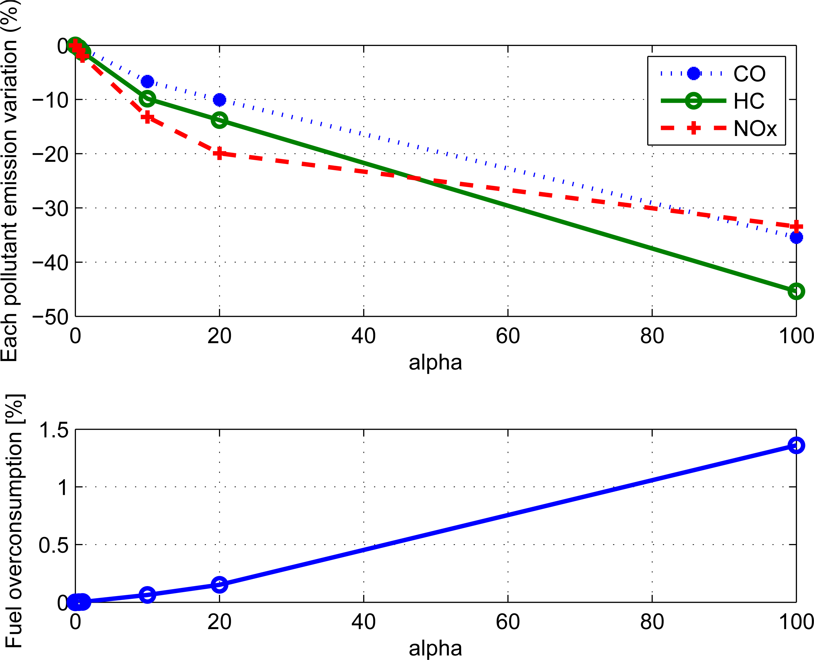
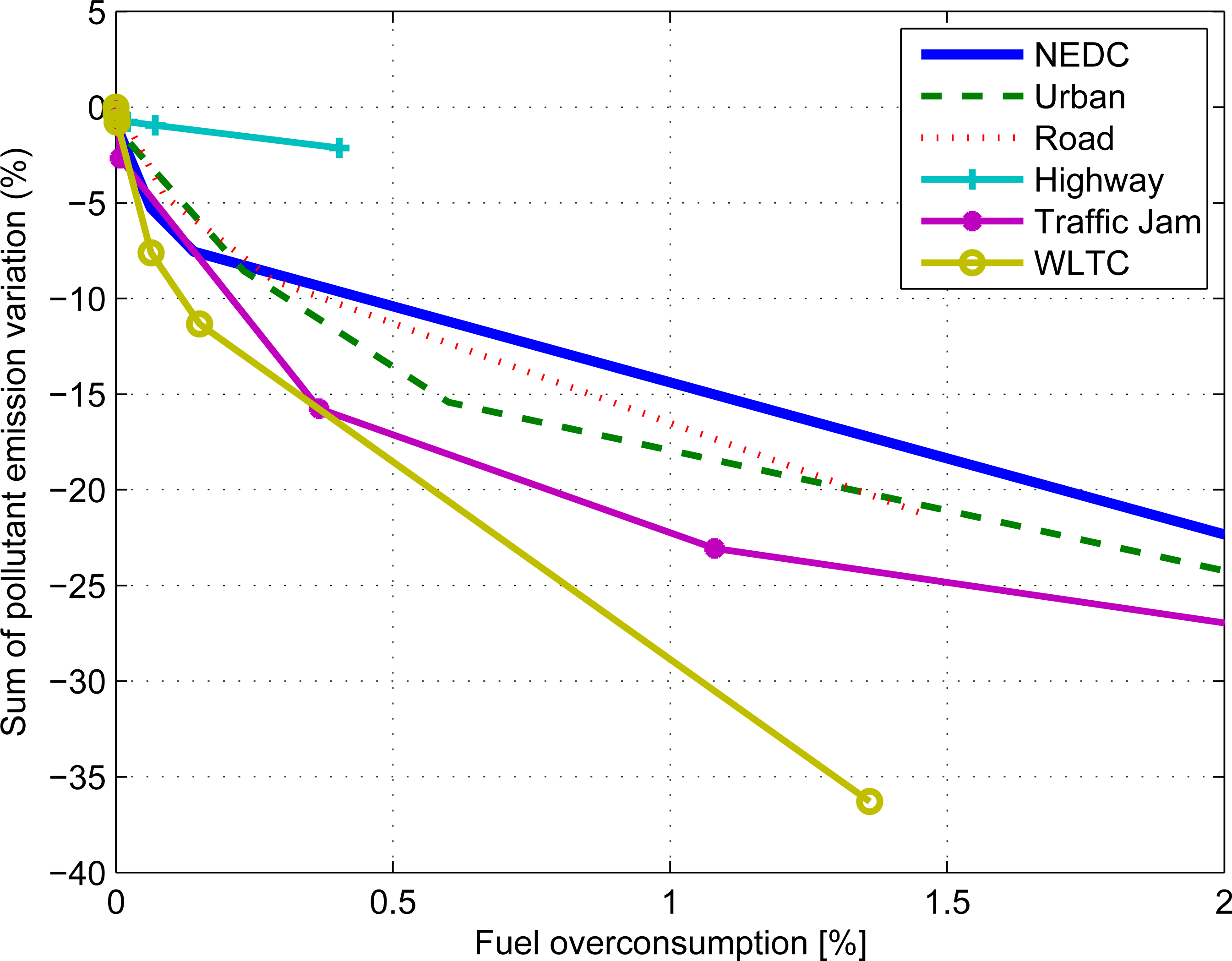
Simulation results are based on a quasi-static model of a parallel gasoline hybrid vehicle. The first result (Figure 1) shows that when α increases, the fuel consumption increases when pollutant emissions decrease for the WLTC (Worldwide Harmonized Light Vehicles Test Cycle). Figure 2 shows that this trade-off between fuel consumption and pollutant emission exists for different driving cycles.

Finally, the fuel consumption minimization with pollution constraint does not require considering directly the 3WCC temperature in the minimization method. However, the catalytic temperature needs to be estimated in order to compute the flows of each pollutant. The same principle will be applied to take into account battery temperature dynamics in the minimization problem in the next section.

3.2. Battery Temperature Constraint

3.2.1. Problem

The battery is often considered as the centerpiece of a hybrid electric application, especially for PHEV, mainly because of its substantial cost and the fact that its performances fades over time. Matching the battery and vehicle lifetimes is a crucial issue in improving the economic viability of HEV. Again, the stake is even higher for PHEV, which rely significantly more on electric energy. If used properly, the degree(s) of freedom offered by hybrid powertrains can contribute to slowing down aging mechanisms by avoiding as much as possible the operating conditions that are harmful to the battery. While several authors have submitted interesting ideas to take battery health into account in the EMS [18,19], the issue remains unresolved.

Battery aging is monitored by the onboard battery management system (BMS) and is commonly expressed as a non-dimensional parameter, the state of health (SOH) [20], decreasing from one (brand new) to zero (worn out) as the battery wears. The aging process of Li-ion batteries is very intricate and is currently the subject of many studies [21–23]. The primary factors enhancing battery aging are high temperatures and high states of charge. The strategy presented in this paper therefore includes a penalty regarding undesired battery temperatures in the optimality criterion. The objective is to combine energy and thermal management and, thus, to ensure a trade-off between powertrain efficiency and battery aging via a soft constraint on cell temperature [24].

3.2.2. Battery Model

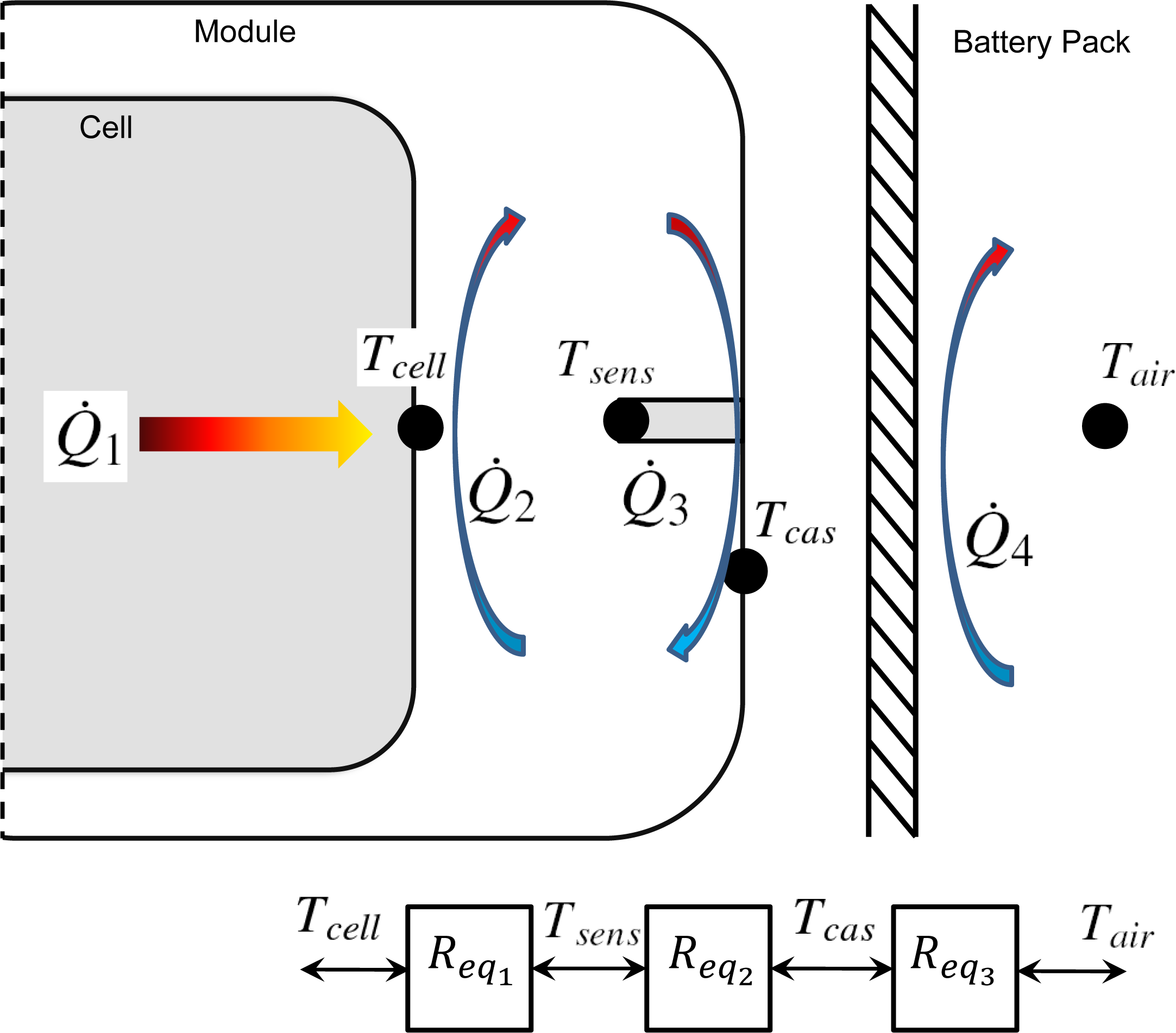
To implement a battery thermal management strategy, a control-oriented model of the battery cells’ temperature has to be designed. The zero-dimensional model considered is based on the heat transfer equations between a cell and the air surrounding the battery pack [25]. The main assumption is a homogeneous temperature of the cells. A depiction of the model’s heat transfers is given in Figure 3. The prismatic cells are enclosed in modules composing the battery pack. As a result, four temperatures are considered: T_cell is the cell temperature, T_sens is the temperature of the air confined in the module, which is given by a sensor on an actual battery pack, T_cas is the temperature of the module casing and, finally, T_air is the air temperature around the battery pack. The temperature model presented in [26]is based on a similar approach, but applied to cylindrical cells and using an observer to consolidate the estimation. For more details about the battery model used, see [24,27].

In order for the energy management strategy to be consistent with PHEV operations, the state of energy (SOE) approach is favored over the classical state of charge calculation [28]. While the SOC is a fair representation of the energy remaining in the battery when considering charge sustaining operation, it is no longer the case for high depletion conditions. For HEV, the SOC is sustained around 50%, where the open circuit voltage (OCV) of the battery is almost constant. Battery current and power flow can therefore be considered proportional. As for a PHEV, the OCV decreases significantly with charge depletion; consequently, current cannot be considered a faithful image of power flow. Ultimately, the charge remaining in the battery is not an accurate estimation of the energy left, which is an important piece of information to assess the electric range of a PHEV. The SOE is defined by:

$$\mathit{SOE}(P_{\mathit{bat}},\mathit{SOC})=\frac{E_R\left(P_{\mathit{bat}},\mathit{SOC}\right)}{E_N}$$

(16)

where E_R is the energy remaining in the battery, P_bat the reversible electric power exchanged with the battery and E_N = OCV_Max; Q_Max is its nominal energy capacity (when fully charged).

3.2.3. New Criterion

As in the previous section for pollutant emission Criterion (12) with Criterion (13), a new cost function J_aging is proposed with an additional cost on battery temperature evolution in addition to the fuel consumption:

$$\begin{array}{ll}{J}_{\mathit{aging}}=\hfill & {\int }_{t_0}^{t_f}\left\{\begin{array}{c}{\dot{m}}_f(u(t),T_{\mathit{wheel}}(t))\\ \mathit{+}{\kappa }_{\mathit{batt}}(T_{\mathit{cell}}){\dot{T}}_{\mathit{cell}}(u(t),T_{\mathit{cell}})\end{array}\right\}dt\hfill \\ \hfill & +\mathrm{\Phi }\left(\mathit{SOE}(t_f)\right)+\mathrm{\Psi }\left(T_{\mathit{cell}}(t_f)\right)\hfill \end{array}$$

(17)

with:

$$\begin{array}{lll}\mathrm{\Phi }\left(\mathit{SOE}(t_f)\right)\hfill & =\hfill & \{\begin{array}{ll}0\hfill & \text{if}\hspace{0.17em}\hspace{0.17em}\mathit{SOE}(t_f)\ge {\mathit{SOE}}_{\mathit{final}}\hfill \\ \infty \hfill & \text{else}\hfill \end{array}\hfill \\ \mathrm{\Psi }\left(T_{\mathit{cell}}(t_f)\right)\hfill & =\hfill & 0\hfill \end{array}$$

(18)

where ṁ_f is the instantaneous fuel consumption, u is the control variable and T_wheel is wheel torque request, imposed by the driver or a driving cycle (speed profile). Ṫ_cell is the cell temperature fluctuation, and κ_batt is a weighting parameter depending on the cell temperature, as represented in Figure 4. The chosen control variable u = P_bat is the power delivered by the battery, which has to be optimized by the EMS to minimize the criterion J_aging. Φ(SOE(t_f)) is a function ensuring a solution meeting the final requirement on the SOE. The final SOE will be chosen equal to its initial value for sustaining operation, but will be close to the minimal SOE admissible by the battery for depleting operation. The function Ψ(T_cell(t_f)) is set to zero, since no constraint is considered for the cell’s final temperature. The above system has two state variables:

$$\mathbf{x}=\left\{\begin{array}{c}\mathit{SOE}\\ T_{\mathit{cell}}\end{array}\right\}$$

the SOE and battery cell temperature. Their dynamics are described in [24].

Under some hypothesis (a lack of constraint on the final cell temperature, very slow cell temperature dynamics), the corresponding Hamiltonian of Criterion (17) can be written:

$$H\left(u,\mathbf{x},T_{\mathit{wheel}},{\lambda }_{\mathit{SOE}}\right)={\dot{m}}_f(u,T_{\mathit{wheel}})+{\lambda }_{\mathit{SOE}}S\dot{O}E(u)+{\kappa }_{\mathit{batt}}(T_{\mathit{cell}}){\dot{T}}_{\mathit{cell}}(u)$$

(19)

In practice, at each sampling time, the command u = P_bat is meshed between the minimum and maximum battery power tolerated by the powertrain, and the value minimizing Equation (19) is chosen as the optimal command u_opt(t) (Equation (10)). The process must be repeated for each time step of the simulation.

The key idea behind this additional cost is to penalize the commands causing the battery temperature to get further away from its slow-aging operating range and to favor the ones that get the temperature closer. The weighting factor κ_batt will allow a trade-off between fuel consumption and safe battery temperature. Setting κ_batt to zero when the battery operates in its slow-aging zone, there will be no additional cost and only fuel consumption will be minimized. On the other hand, κ_batt increases when the temperature gets past the slow-aging zone, the higher the temperature, the higher the cost, to prevent the temperature from rising further. On the opposite, the negative cost caused by negative values of κ_batt when the temperature is too cold favors battery warming, once again to get it closer to the slow-aging zone.

3.2.4. Results

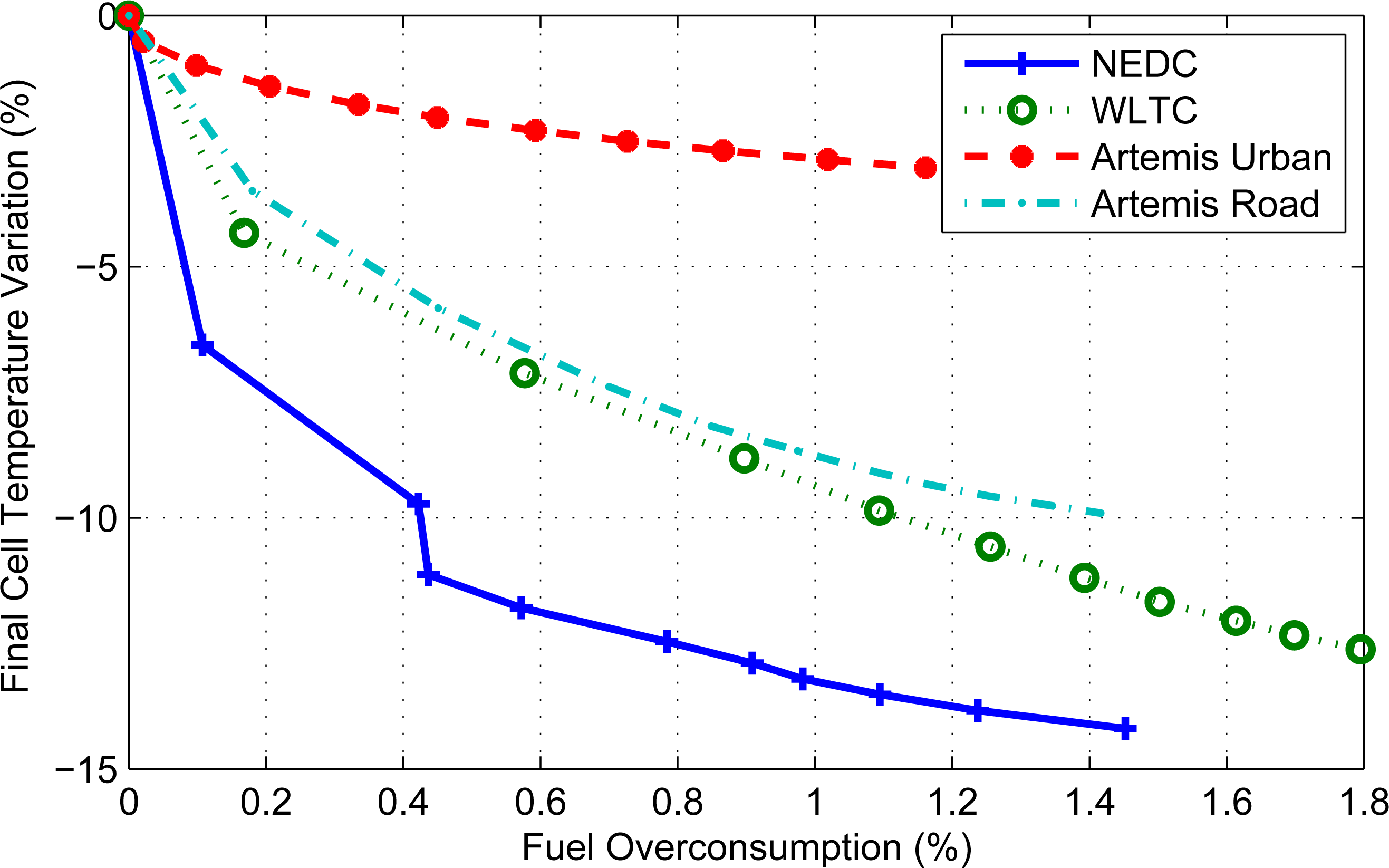
The PHEV considered is provided with a parallel hybrid powertrain. Simulation results are based on a quasi-static model of the vehicle and powertrain. The vehicle’s dynamics is given by Newton’s second law. As for the hybrid powertrain, engine, electrical machine and battery efficiencies are computed using look-up tables. The considered scenario is based on charge sustaining operation in normal weather; the external air temperature (and initial cell temperature) is set to 25 °C and κ_batt = 0 between 0 °C and 25 °C. The trip is made of a succession of the chosen cycles; the total length of the trip is 80 km. SOE is controlled around 50% with a proportional integral control on the λ_SOE as in a real vehicle. Figure 5 displays the decrease in the cell temperature (%) as a function of the fuel overconsumption (%). It shows a trade-off curve between battery health through cell temperature decrease and fuel consumption. The same principle will be applied to take into account drivability in the minimization problem in the next section.

3.3. Drivability Constraint

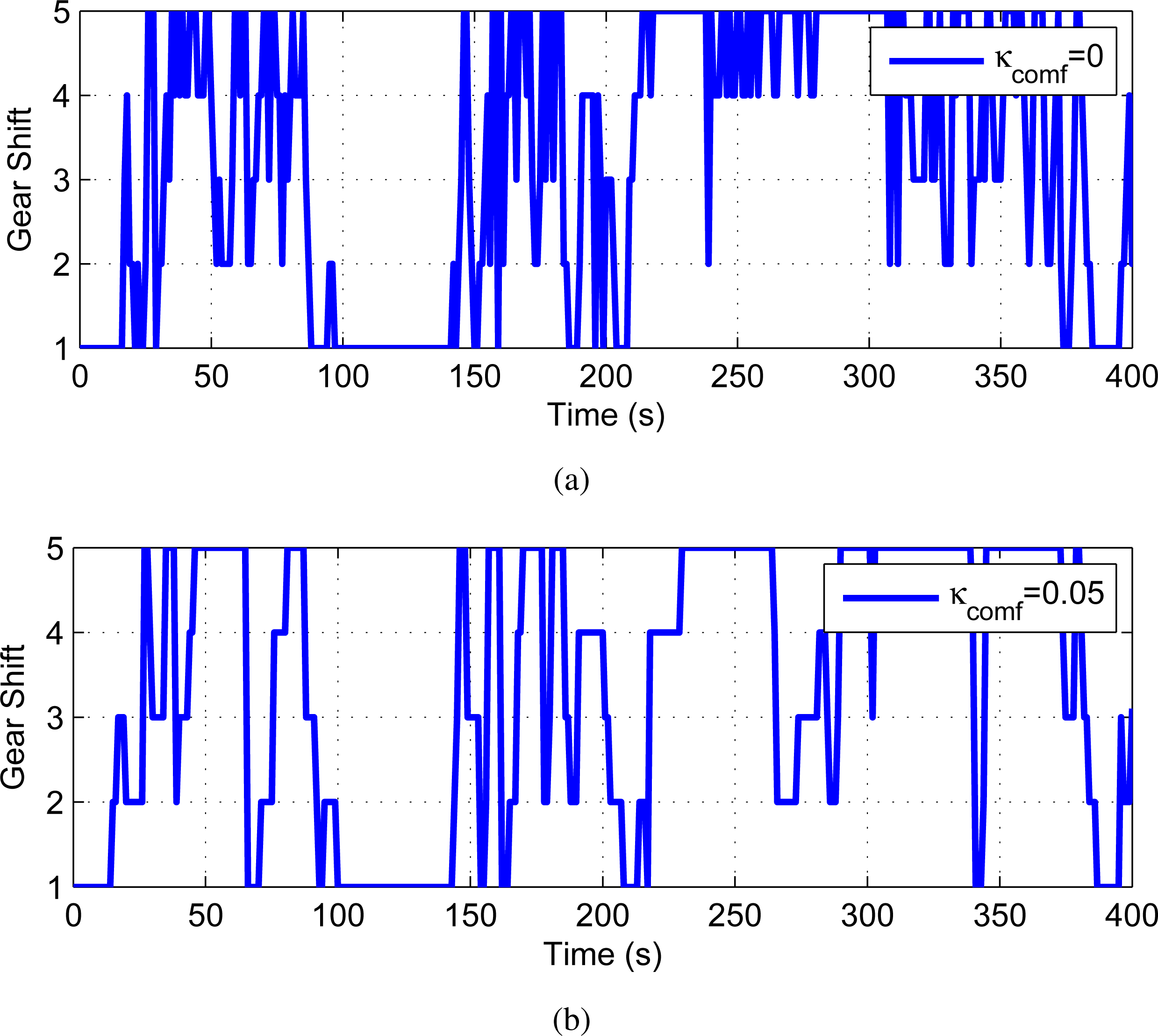
As previously mentioned, the historical objective of EMS was to minimize fuel consumption only. However, classical ECMS gives an erratic control behavior, especially when considering gear shifting in the control vector (the top of Figure 6).

The problem of defining comfort is not straightforward, and studies, such as [6], show that simpler criteria could be used in the EMS. Unlike fuel consumption, which can be easily evaluated, drivability is fairly subjective. However, to assess the performance of a strategy and also the tradeoff between fuel consumption and drivability, it is necessary to quantify drivability based on specific behaviors. The most common metrics are the number of events (or mean dwell time) on engine and gear states. Let us define a generic criterion for discomfort:

$$\mathit{Discomfort}=\frac{1}{d_{\mathit{cycle}}}\sum _{k=1}^{k_{\mathit{final}}-1}\beta \left(M_k^{\mathit{cin}},M_{k+1}^{\mathit{cin}}\right)$$

(20)

where k is the discrete time, d_cycle is the cycle distance (m) and β a matrix of weights that are a function of the kinematic mode M^cin (e.g., gear shifting) that can be equal to $\left|M_k^{\mathit{cin}}-M_{k+1}^{\mathit{cin}}\right|$ as in [6], ${\left(M_k^{\mathit{cin}}-M_{k+1}^{\mathit{cin}}\right)}^2$ as in [7]. The proposed methodology is to attribute a higher penalty to transitions most inconvenient for the driver, implying, for example, torque interruption, jerk, engine start, etc. On the contrary, the more a transition is unnoticeable for the driver, the lowest its penalty may be. Here, β, which could be considered as a specific penalty for each possible transition, is a combination of engine events and gear events.

3.3.1. New Criterion

As shown in the two previous sections for other constraints, the Hamiltonian can be simply penalized by an additional cost. Hence, to take into account the drivability constraint, a new Hamiltonian function H_comf is proposed with an additional cost on discomfort that multiplies the classical Hamiltonian H_energ (Equation (11)):

$$H_{\mathit{comf}}=H_{\mathit{energ}}+{\kappa }_{\mathit{comf}}\left|\beta \left(M_k^{\mathit{cin}},M_{k+1}^{\mathit{cin}}\right)H_{\mathit{energ}}\right|$$

(21)

where κ_comf is the tunable constant.

3.3.2. Results

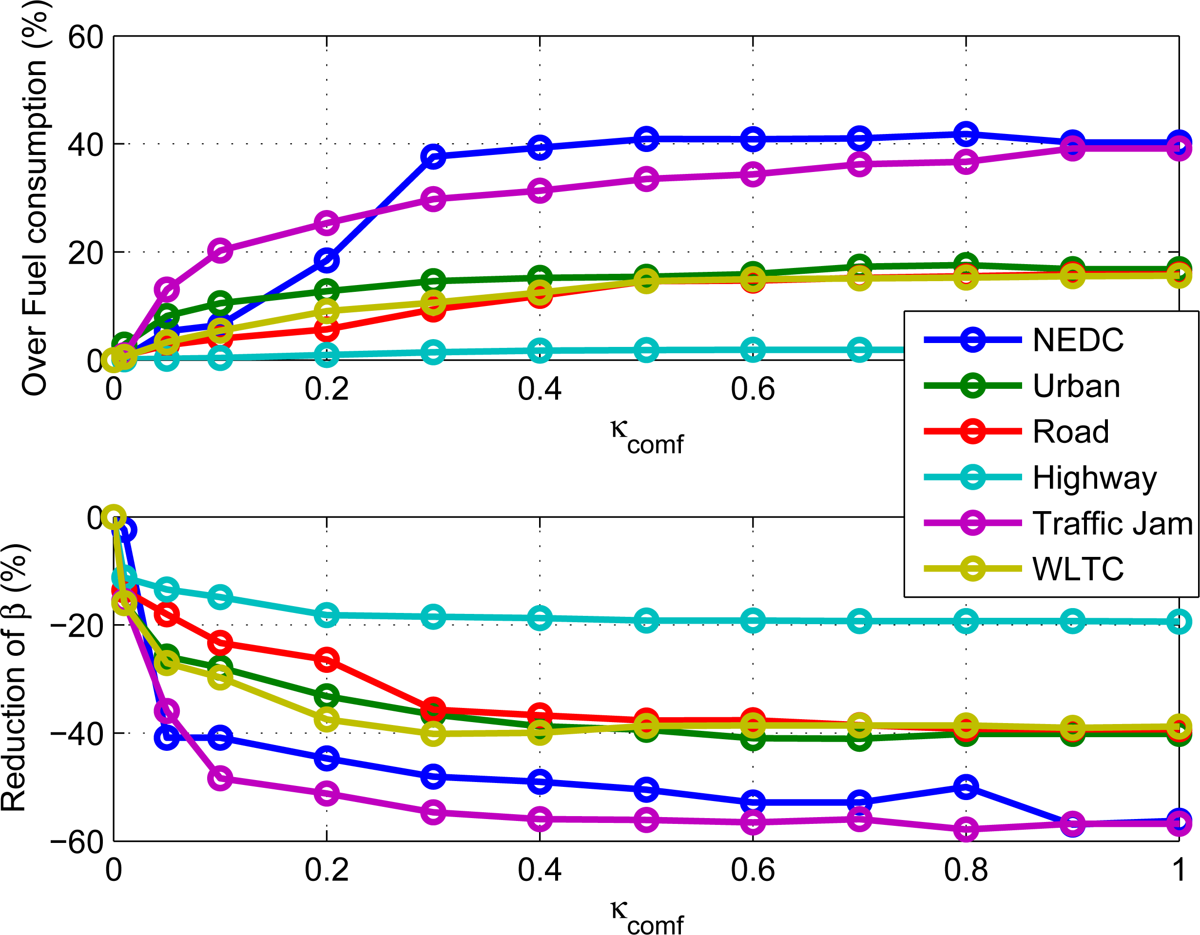
Simulation results are based on a quasi-static model of the vehicle and powertrain with five modes. As shown at the bottom of Figure 6, the new Hamiltonian decreases mode shifting. The first study shows that increasing κ_comf increases comfort (Figure 7) for different cycles (New European Driving Cycle, Artemis cycles and Worldwide Harmonized Light Vehicles Test Cycle).

Moreover, as previously mentioned, only a simpler variable κ_comf permits one to decrease every drivability metrics (

Table 1. Drivability metrics on the WLTC (Worldwide Harmonized Light Vehicles Test Cycle) for different values of κ_comf.

κcomf	0	0.01	0.05	0.1	1
Gear events	442	316	262	266	191
Engine events	150	140	120	114	102
Mean dwell time (s)	4.1	5.7	6.8	6.9	9.4
Events lasting less than 4 s	81	9	5	2	1
Extra fuel consumption (%)	0	0.6	3.28	5.4	15.6

). The extra fuel consumption is computed with respect to κ_comf = 0.

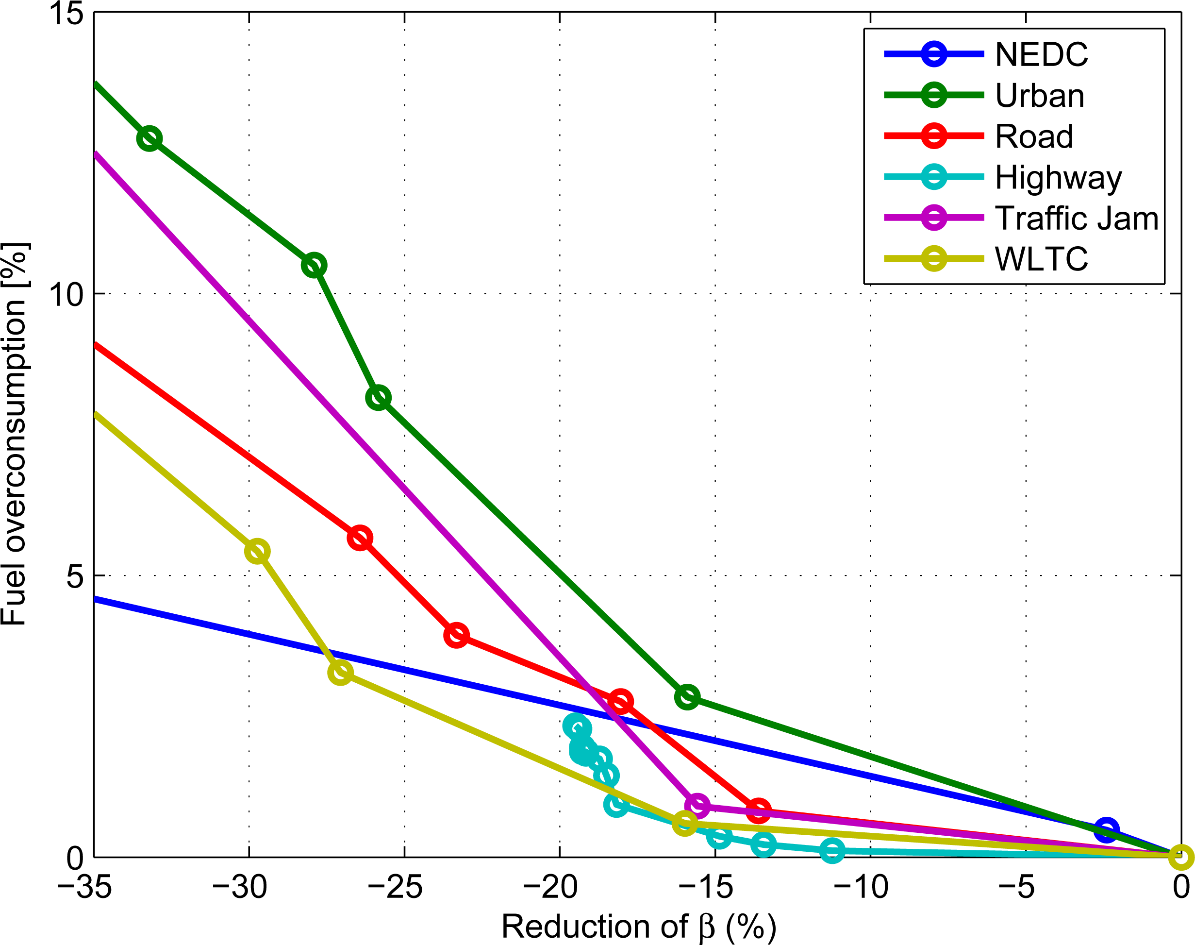
Hence, the use of this new Hamiltonian provides a solution that is easily tunable, as shown in Figure 8 for different cycles. Moreover, it is shown that a trade-off between fuel consumption and comfort exists.

3.4. Drivability and Pollutant Emissions Constraints

In Sections 3.1 and 3.3, it was shown that constraints on pollutant emission or drivability can be taken separately. In this section, we will show that we can take both constraints into account at the same time in the energy management strategy. Hence, by grouping Equations (13), (14) and (21), the new Hamiltonian H_mix becomes:

$$H_{\mathit{mix}}=H_{\mathit{pollu}}+{\kappa }_{\mathit{comf}}\left|\beta \left(M_k^{\mathit{cin}},M_{k+1}^{\mathit{cin}}\right)H_{\mathit{pollu}}\right|$$

(22)

with:

$$H_{\mathit{pollu}}={\dot{m}}_f(u(t),t)+\alpha \sum _i\frac{{\dot{m}}_{\mathit{ex}{\mathit{h}}_i}\left(u(t),T_{\mathit{cata}}(t),t\right)}{{\sigma }_i}+{\lambda }_1(t)S\dot{O}C$$

(23)

where κ_comf is the tunable constant on the drivability and where α is the tunable constant on the pollutant emission.

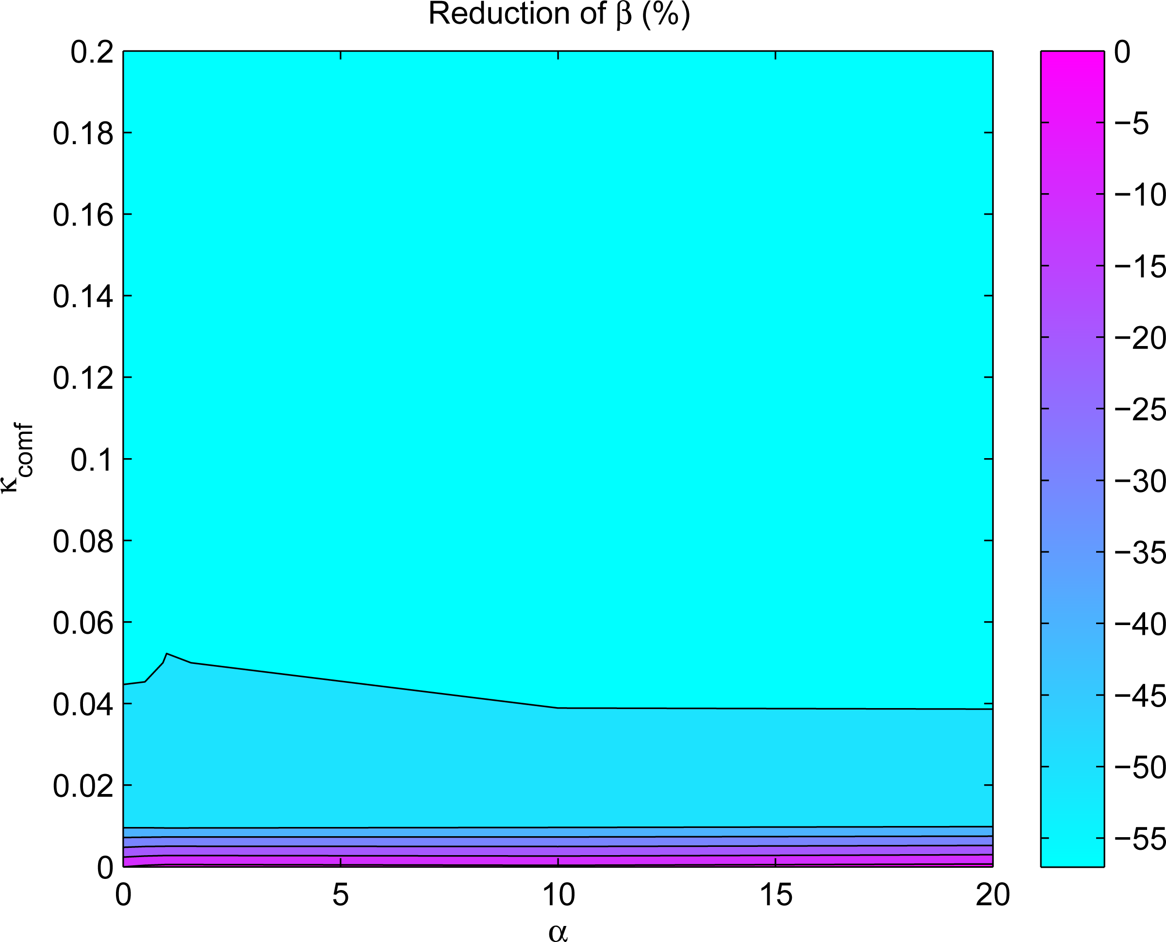
Figures 9 and 11 show the simulation results with a quasi-static model of the vehicle and powertrain with five modes and a one-dimensional model for the catalytic temperature [29]. The simulation results are charge sustaining constrained, with a binary search of the constant λ₁ (Equation (23)). In each figure, the variation of β, pollutant emission or fuel consumption are shown relative (%) to the value computed for α = κ_comf = 0 (reference point). Figure 9 shows that the comfort increases for each value of α. Indeed, β decreases exponentially when κ_comf increases for any value of α, as shown previously in Figure 7 for α = 0. It can be noticed that α has a negligible influence on the drivability.

Figure 10 shows that the pollutant emissions decrease when α increases for each value of κ_comf. Here, κ_comf has a great influence on the vehicle pollutant emissions, so that in order to maintain the pollutant emissions to the level without drivability (with κ_comf = 0), the value of α must increase. For example, to get the same amount of pollutant emission as α = κ_comf = 0 for κ_comf = 0.2, the value of α must be set to 10.

Finally, as the constraint parameters κ_comf and α increase, fuel consumption increases (Figure 11), so that a trade-off appears between fuel consumption, comfort and pollutant emissions. Note that the choice for the couple {α, κ_comf} is guided by:

• a minimum and maximum frequency of gear/engine events, represented by the iso-lines of Figure 9;

• the pollution standard, represented by an iso-line of Figure 10, that must not be exceeded;

• the maximum allowed fuel consumption, represented by an iso-line of Figure 11. For example, a compromise setting could be α =20 and κ_comf = 0.05.

4. Conclusions

From these examples, it seems possible to find an energy management strategy that takes into account a constraint (drivability, pollutant emissions, aging, environment). However, taking these constraints into account is made to the detriment of fuel consumption (the existence of a trade-off). This trade-off may sometimes be difficult to find, and it increases the complexity of the optimization problem, but the generic tools developed in this paper should help to find an acceptable solution quickly.

References

- Sciarretta, A.; Back, M.; Guzzella, L. Optimal control of parallel hybrid electric vehicles. IEEE Trans. Control Syst. Technol 2004, 12, 352–363. [Google Scholar]
- Rousseau, G.; Sciarretta, A.; Sinoquet, D. Optimal energy management of a mild-hybrid vehicles. In Proceedings of the 4th European Conference on Alternative Energies for the Automotive Industry, Futuroscope-Poitier, France, 2–3 April 2008.
- Delprat, S.; Laubert, J.; Guerra, T.; Rimaux, J. Control of a parallel hybrid powertrain: Optimal control. IEEE Trans. Veh. Technol 2004, 53, 872–881. [Google Scholar]
- Johnson, V.; Wipke, K.; Rausen, D. HEV Control Strategy for Real-Time Optimization of Fuel Economy and Pollutant Emissions; SAE Technical Paper 2000-01-1543; Society of Automotive Engineers, Inc.: Warrendale, PA, USA; 2; April; 2000. [Google Scholar]
- Michel, P.; Charlet, A.; Colin, G.; Chamaillard, Y.; Bloch, G.; Nouillant, C. Pollution constrained optimal energy management of a gasoline-HEV. In Proceedings of the 11th International Conference on Engines and Vehicles, ICE, Capri, Italy, 15–19 September 2013.
- Opila, D.; Aswani, D.; McGee, R.; Cook, J.; Grizzle, J. Incorporating drivability metrics into optimal energy management strategies for hybrid vehicles. Proceedings of the IEEE Conference on Decision and Control, Cancun, Mexico, 9–11 December 2008.
- Debert, M.; Padovani, T.M.; Colin, G.; Chamaillard, Y.; Guzzella, L. Implementation of comfort constraints in dynamic programming for hybrid vehicle energy management. Int. J. Veh. Des 2012, 58, 367–386. [Google Scholar]
- Sunström, O.; Guzzella, L.; Soltic, P. Optimal hybridization in two parallel hybrid electric vehicles using dynamic programming. In Proceedings of the 17th World Congress of the International Federation of Automatic Control, Seoul, Korea, 6–11 July 2008.
- Lin, C.; Kang, J.; Grizzle, J.; Peng, H. Energy management strategy for a parallel hybrid electric truck. Proceedings of the 2001 American Control Conference, Arlington, VA, USA, 25–27 June 2001; pp. 2878–2883.
- Guzzella, L.; Sciarretta, A. Vehicle Propulsion Systems: Introduction to Modeling and Optimization; Springer: Berlin, Germany, 2005. [Google Scholar]
- Pontryagin, L.S.; Boltyanskii, V.; Gamkrelidze, R.; Mischchenko, E. The Mathematical Theory of Optimal Processes; Interscience: New York, NY, USA, 1962. [Google Scholar]
- Sciarretta, A.; Guzzella, L.; Back, M. A real-time optimal control statement for parallel hybrid vehicles with on-board estimation of control parameters. In Proceedings of the IFAC Symposium Advance in Automotive Control, Salerno, Italy, 19–23 April 2004; pp. 502–507.
- Chasse, A.; Pognant-gros, P.; Sciarretta, A. Online implementation of an optimal supervisory control for a parallel hybrid powertrain. SAE Int. J. Engines 2009, 2, 1630–1638. [Google Scholar]
- Johannesson, L. Predictive Control of Hybrid Electric Vehicles on Prescribed Routes. Ph.D. Thesis, Chalmers University of Technology, Gothenburg, Sweden. 2009. [Google Scholar]
- Ambühl, D.; Sciarretta, A.; Onder, C.; Guzzella, L.; Sterzing, S.; Mann, K.; Kraft, D.; Küsell, M. A causal operation strategy for hybrid electric vehicules based on optimal control theory. Proceedings of the 4th Symposium Hybrid Vehicles and Energy Management, Braunschweig, Germany, 14–15 February 2007.
- Sivertsson, M.; Sundström, C.; Eriksson, L. Adaptive control of a hybrid powertrain with map-based ECMS. Proceedings of the 18th World Congress of the International Federation of Automatic Control (IFAC), Milano, Italy, 28 August–2 September 2011.
- Serrao, L.; Sciarretta, A.; Grondin, O.; Chasse, A.; Creff, Y.; di Domenico, D.; Pognant-Gros, P.; Querel, C.; Thibault, L. Open issues in supervisory control of hybrid electric vehicles: A unified approach using optimal control methods. Proceedings of the International Scientific Conference on Hybrid and Electric Vehicles, RHEVE, Rueil-Malmaison, France, 6–7 December 2011.
- Serrao, L.; Onori, S.; Sciarretta, A.; Guezennec, Y.; Rizzoni, G. Optimal energy management of hybrid electric vehicles including battery aging. Proceedings of the 2011 American Control Conference, San Francisco, CA, USA, 29 June–1 July 2011.
- Ebbesen, S.; Elbert, P.; Guzzella, L. Battery state-of-health perceptive energy management for hybrid electric vehicles. IEEE Trans. Veh. Technol 2012, 61, 2893–2900. [Google Scholar]
- Remmlinger, J.; Buchholz, M.; Meiller, M.; Bernreuter, P.; Dietmayer, K. State-of-health monitoring of lithium-ion batteries in electric vehicles by on-board internal resistance estimation. J. Power Sources 2011, 196, 5357–5363. [Google Scholar]
- Gyan, P.; Aubret, P.; Hafsaoui, J.; Sellier, F.; Bourlot, S.; Zinola, S.; Badin, F. Experimental assessment of battery cycle life within the SIMSTOCK research program. Oil Gas Sci. Technol. Rev. IFP Energies nouvelles 2013, 68, 137–147. [Google Scholar]
- Vetter, J.; Novak, P.; Wagner, M.; Veit, C.; Möller, K.C.; Besenhard, J.; Winter, M.; Wohlfart-Mehrens, M.; Vogler, C.; Hammouche, A. Ageing mechanisms in lithium-ion batteries. J. Power Sources 2005, 147, 269–281. [Google Scholar]
- Broussely, M.; Biensan, P.; Bonhomme, F.; Blanchard, P.; Herreyre, S.; Nechev, K.; Staniewicz, R. Main aging mechanisms in Li ion batteries. J. Power Sources 2005, 146, 90–96. [Google Scholar]
- Miro-Padovani, T.; Debert, M.; Colin, G.; Chamaillard, Y. Optimal energy management strategy including battery health through thermal management for hybrid vehicles. Proceedings of the 7th IFAC Symposium on Advances in Automotive Control, AAC, Tokyo, Japan, 4–7 September 2013.
- Muratori, M.; Canova, M.; Guezennec, Y.; Rizzoni, G. A reduced-order model for the thermal dynamics of Li-ion battery cells. Proceedings of the 6th IFAC Symposium Advances in Automotive Control, Munich, Germany, 11–14 July 2010; pp. 192–197.
- Lin, X.; Perez, H.E.; Siegel, J.B.; Stefanopoulou, A.G.; Li, Y.; Anderson, R.D.; Ding, Y.; Castanier, M.P. Online parameterization of lumped thermal dynamics in cylindrical lithium ion batteries for core temperature estimation and health monitoring. IEEE Trans. Control Syst. Technol 2013, 21, 1745–1755. [Google Scholar]
- Debert, M.; Colin, G.; Bloch, G.; Chamaillard, Y. An observer looks at the cell temperature in automotive battery packs. Control Eng. Pract 2013, 21, 1035–1042. [Google Scholar]
- Stockar, S.; Marano, V.; Canova, M.; Rizzoni, G.; Guzzella, L. Energy-optimal control of plug-in hybrid electric vehicles for real-world driving cycles. IEEE Trans. Veh. Technol 2011, 60, 2949–2962. [Google Scholar]
- Michel, P.; Charlet, A.; Colin, G.; Chamaillard, Y.; Bloch, G.; Nouillant, C. Catalytic converter modeling for optimal gasoline-HEV energy management. Proceedings of the 19th World Congress of the International Federation of Automatic Control, Cap Town, South Africa, 24–29 August 2014.