Article

Estimating the Technical Improvement of Energy Efficiency in the Automotive Industry—Stochastic and Deterministic Frontier Benchmarking Approaches

by
Seog-Chan Oh
1,*,† and
Alfred J. Hildreth
2,†
1
General Motors Research and Development, 30500 Mound Road, Warren, MI 48090, USA
2
General Motors, 30200 Van Dyke, Warren, MI 48090, USA
*
Author to whom correspondence should be addressed.
These authors contributed equally to this work.
Energies 2014, 7(9), 6196-6222; https://doi.org/10.3390/en7096196
Submission received: 10 July 2014 / Accepted: 15 September 2014 / Published: 25 September 2014

Abstract

:
The car manufacturing industry, one of the largest energy consuming industries, has been making a considerable effort to improve its energy intensity by implementing energy efficiency programs, in many cases supported by government research or financial programs. While many car manufacturers claim that they have made substantial progress in energy efficiency improvement over the past years through their energy efficiency programs, the objective measurement of energy efficiency improvement has not been studied due to the lack of suitable quantitative methods. This paper proposes stochastic and deterministic frontier benchmarking models such as the stochastic frontier analysis (SFA) model and the data envelopment analysis (DEA) model to measure the effectiveness of energy saving initiatives in terms of the technical improvement of energy efficiency for the automotive industry, particularly vehicle assembly plants. Illustrative examples of the application of the proposed models are presented and demonstrate the overall benchmarking process to determine best practice frontier lines and to measure technical improvement based on the magnitude of frontier line shifts over time. Log likelihood ratio and Spearman rank-order correlation coefficient tests are conducted to determine the significance of the SFA model and its consistency with the DEA model. ENERGY STAR® EPI (Energy Performance Index) are also calculated.

1. Introduction

The growing awareness of global energy demand issues has become one of major contributors to create the concept of sustainability. According to International Energy Agency, the average energy use per person has increased 10%, while the world population has increased 27% from 1990 to 2008. Energy-related CO2 emissions are expected to rise from an estimated 31.2 Gt in 2011 to 37.0 Gt in 2035. The concept of sustainability was first used to describe an economic vision in equilibrium with basic ecological support systems in the 1970s. The concept has since been applied to a wide range of areas, including the car manufacturing industry, thus, motivating the change in energy consumption trends.
The typical vehicle manufacturing plants of car companies consume energy at different rates, depending on many external or internal factors, such as plant utilization, heating degree days (HDD) and cooling degree days (CDD), which are positively correlated to such factors as heating and cooling energy requirements, product type and size. Although car companies recognize that energy consumption is a large but mandatory expense, most of them have recently invested in energy saving initiatives for their plants every year to reduce energy consumption inspired by the concept of sustainability and its implication for firm values such as enhanced brand value or cost savings in energy. A notable fact is that those energy saving initiatives have been, in many cases, supported by government research or financial programs (e.g., R&D and funding programs offered by US Department of Energy Office of Energy Efficiency and Renewable Energy) because those initiatives are also aligned with the government’s energy saving polices. The benefits from energy demand reduction could be significant, ranging from energy conservation and reduced environmental impact to an enhanced competitive position.
Regarding the energy use associated with the U.S. automotive enterprise, over 200 trillion BTU (British thermal units) per year has been roughly estimated, as shown in Figure 1 (note: auto-manufacturing industries include motor vehicle manufacturing, motor vehicle body and trailer manufacturing, and motor vehicle parts manufacturing classified in NAICS (North American Industry Classification System). However, if a complex supply chain is included in calculating the contribution, the total energy consumption related to the car manufacturing industry will be considerably greater, as the complex supply chain includes the following: producing raw materials, such as steel, aluminum, plastics, and glass; forming and fabricating parts, components, and subsystems; assembling hundreds of these elements to manufacture the vehicles; and distributing and selling the vehicles.
Table 1 summarizes and compares the intensity of utility use (e.g., electricity/vehicle, fuel/vehicle and water/vehicle) and carbon emission to produce one vehicle among major car companies. Note that Scopes 1 and 2 refer to the direct emissions by the firm at its installations and to the indirect emissions by the firm through electricity use, respectively. Scope 3 often refers to supply chain emissions. Some car making companies report their Scope 3 emissions to the Carbon Disclosure Project (CDP), which is an independent organization supported by major institutional investors. Note that the energy data in this section are based on on-site energy consumption except that the flow diagram in Figure 1 is based on the source Btu and the carbon emission amount in Scopes 1 and 2 emission types in Table 1 includes the indirect emission for purchased utilities in the energy generation sites.
Figure 2 depicts the magnitude of total energy consumption in the car manufacturing industry compared to Boeing and major US government agencies; as shown, energy consumption in the car manufacturing industry is considerably greater, with the exception of the U.S. Department of Defense, with an energy consumption of approximately 900 trillion BTU.
Figure 1. Energy flows into the US auto manufacturing industry 2011 (data sources: [1,2]).
Energies 07 06196 g001
Figure 2. Energy consumption in auto manufacturing industries in 2011.
Energies 07 06196 g002
Table 1. Resources used to manufacture a vehicle (2012).
Intensity (Use per Vehicle)General MotorsVolkswagenFordBMWToyota (North America)Equivalence
Energy (Electricity + Fuel) Mwh/Vehicle2.302.212.452.442.13Energy for the production of 4 vehicles equals approximately the average annual electricity consumption for a U.S. residential utility customer
Carbon (Scopes 1 & 2) Ton/Vehicle0.880.890.90.680.78Carbon emitted from the production of 1 vehicle equals approximately the carbon offset of 80 trees grown for 10 years
Water m3/Vehicle4.624.554.32.13.41Water for the production of 1 vehicle is similar to that required to fill a small pool
Data sourceGM Sustainability Report [3]Volkswagen Sustainability Report [4]Ford Sustainability Report [5]BMW Sustainability Report [6]Toyota North American Environmental Report [7]Note: the average annual electricity consumption for a U.S. residential utility customer was 11,280 kWh, an average of 940 kWh per month according to U.S. Energy Information Administration in 2011
Although the total energy consumption is large, the energy intensity of the car manufacturing industry is not so large. When energy intensity is calculated as the share of total energy expenditures (electricity and fuel) as a fraction of total operating expenditures (the sum of materials’ costs, labor compensation and new capital expenditures), the U.S. motor vehicle manufacturing industry (NAICS code: 3361) is merely 0.4%, compared to other energy intensive industry. For example, the energy intensity of the U.S. lime manufacturing (32741) and the U.S. industrial gas manufacturing industries (32512) is 37.15% and 34.60%, respectively.
Nonetheless, as the benefits from reducing energy demand are significant, many car companies have invested considerably in strategic energy saving initiatives with the support of government R&D or financial subsidies. Now, as a logical following step, car companies and the government endeavor to investigate whether the implemented energy saving initiatives have been effective and further, institutionalized as a managed process or as a part of organizational capability because they seek to determine whether their investment or subsidies were justified and whether they have been recovered. An industry or a company, if the energy saving initiative are implemented and fully institutionalized, starts to have the potential to deliver sustained energy savings, thereby demonstrating best practices in decreasing energy intensity (kWh/vehicle in the context of car manufacturing industry). When the industry or company obtains the potential to deliver sustained energy savings and the potential is expressed as best practices, a structural technical improvement in the industry (or company) is considered to have been made. Therefore, it is possible to use the term technical improvement as a performance indicator to identify the effectiveness of energy saving initiatives, in other words, the extent to which strategic energy saving initiatives become institutionalized or part of organizational standard processes. The challenge is the lack of suitable quantitative methods to measure a structural technical improvement objectively. This paper applies a benchmarking approach to measure technical improvement. A benchmark is a process for identifying best practices in an industry (or a large company controlling many individual producers insides) and estimating each industry’s or company’s efficiency by measuring the difference between actual performance and best practices. In the context of the car manufacturing industry, the difference between the actual energy use at a plant and its best practice, i.e., the lowest achievable energy use, is considered. The problem is that what is the best achievable is influenced by different operating conditions of plants (e.g., heating or cooling energy requirements, product size, or plant utilization), thus, the measuring of best practices must account for these different operation conditions. A suitable benchmark model should normalize these conditions and identify a frontier line that connects the best practices in the industry. This paper utilized a benchmarking approach, with the shifts of a frontier line between the time period from t and t + Δ t used as a proxy to measure a structural technical improvement. Figure 3 depicts the idea process for measuring the effectiveness of energy saving initiatives with a benchmarking process.
This paper aims to determine and to measure the effectiveness of energy reduction initiatives in terms of a technical improvement that corresponds to a certain structural change in industry-wide energy efficiency between two distinct time periods, namely, by proposing benchmarking models: SFA (stochastic frontier analysis) models based on Hicksian neutral technological change concept and DEA (data envelopment analysis) models incorporating the Malmquist Productivity Change Index (Section 3 discusses Hicksian concept and Malmquist index in detail). Through the SFA and DEA benchmarking processes, it is possible to identify best practice frontier lines and to analyze the technical improvement based on the magnitude of the frontier line shifts over time.
Figure 3. The idea process for measuring the effectiveness of energy saving initiatives.
Energies 07 06196 g003
It is possible to more holistically understand the factors affecting energy consumption by checking the consistency of the analytical results from two different models, SFA and DEA [8]. Previous findings from performance benchmarking literature indicate that DEA and SFA have comparative advantages against each other, thereby offering the possibility of complementary use. In general, DEA is preferable in applications in which the frontier model cannot be expressed in algebraic form or does not have a known inefficiency distribution. The SFA method is preferable when certain classical assumptions are satisfied regarding the composite error terms, including the contributions from the inefficiency distribution and measurement errors. Often, SFA and DEA estimates are highly correlated in terms of rank order, regardless of inefficiency and random error variation, meaning that the feasibility and robustness of the model estimation can be demonstrated by showing a high correlation between two models. Hence, in this paper, the Spearman rank correlation is used to check the consistency of two different models. This paper also calculates ENERGY STAR® plant energy performance indicator values based on the SFA models.
The paper is organized as follows: Section 2 surveys some efforts and studies related to energy use in the automotive industry and overviews benchmarking models including parametric and non-parametric approaches. Section 3 describes SFA and DEA and the concept of technical improvement in additional detail with graphics and proposes benchmarking models to assess the significance of technical improvements in energy use alongside background data about energy consumption in vehicle manufacturing processes. Section 4 provides illustrative studies by using hypothetical but representative panel data sets (note: panel data refer to a group of cross-sectional data sets separated into periods of time, thus, appearing as a combination of cross-sectional and time series data sets). For confidentiality reasons, hypothetical data sets are used for the studies. In addition to implementing models, the final proposed models are analyzed and validated. Section 5 concludes the paper. Appendix A shows the resulting parameters obtained from SFA and DEA models. Appendix B summarize the results of comparison between the estimated models in this study and those of previous estimated models.

2. Literature Review

Several studies related to demand, supply and management for energy use in the car manufacturing industry have been conducted.
Galitsky and Worrell [9] collected energy efficiency improvement opportunities available to car manufacturers. They identified many energy efficiency improvement opportunities for each automotive manufacturing operation. Boyd [10] developed plant-level energy performance indicators (EPIs) in support of the Environmental Protection Agency’s ENERGY STAR program in which 35 automotive manufacturing plants of five auto companies had participated. The participating plants were plants having only body welding, assembly and painting operations. Sullivan et al. [11] discussed calculating the environmental burdens of the part manufacturing and vehicle assembly stage of the vehicle life cycle. Their approach is bottom-up, with a particular focus on energy consumption and CO2 emissions. They applied their models to both conventional and advanced vehicles, the latter of which include aluminum-intensive, hybrid electric, plug-in hybrid electric and all-electric vehicles. Oh and Hildreth [12] proposed a novel decision model based on activity based costing (ABC) and stochastic programming that was developed to accurately evaluate the impact of load curtailments and to determine whether to accept an energy load curtailment offer in the smart grid.
Many previous studies on SFA and DEA, as well as the comparison of their differences are available. In research on SFA, Aigner et al. [13] and Meeusen and Broeck [14] proposed the stochastic frontier production function independently. The original model specification considered a production function specified for cross-sectional data in which an error term is divided into two components, one to account for random effects and another to account for technical inefficiency. Subsequently, the original model specification has been used in a large number of empirical applications over the past decades and has also been altered or extended in several ways. One extension is the two-stage estimation procedure to measure the technical change over two time periods in which firm-level efficiencies are predicted using the estimated stochastic frontiers, after which the predicted firm-level efficiencies are regressed upon firm-specific variables (such as managerial skill level change and first decision maker’s characteristics) to distinguish reasons for technical changes over time. However, the two-stage estimation procedure has been criticized because it is inconsistent with its assumptions regarding the independence of the inefficiency effects over two time periods. This paper follows the model specifications proposed by Battese and Coelli [15] that addressed the issues inherent to the two-stage procedure.
Regarding research on DEA, Charnes, Cooper, and Rhodes [16] proposed the constant returns of scale (CRS) restricted DEA model by combining the Farrell efficiency rating concept and a non-parametric mathematical programming better known as CCR (Charnes-Cooper-Rhodes) model, named after its inventors. The CCR model was updated by Banker, Charnes, and Cooper [17], who relaxed the constant returns of scale restriction to be variable returns to scale (VRS), thereby able to evaluate both the technical efficiency and the scale efficiency of decision making units (DMUs). The DEA model with the VRS concept is also called a BCC (Banker-Charnes-Cooper) model, likewise named after its inventors. To implement the VRS concept, the BCC model added an additional constraint to the CCR model, that is, the convexity restriction. When a panel data set is available and one would like to measure the technical improvement using DEA models, the Malmquist total factor productivity (TFP) index can be used to reveal a positive or negative technical change across consecutive years. The Malmquist TFP index [18] requires four distance function values, and each distance function has an equivalent DEA model. This paper discusses those four distance functions in detail in Section 3.3.
Despite the fact that both SFA and DEA methods are benchmarking methods based on efficiency frontier analysis, they differ markedly. SFA is a parametric model that requires a modeler’s assumption in building models. SFA is well suited to separate firms’ inefficiency from statistical noise. By contrast, DEA is a non-parametric model not subject to a modeler’s assumption and useful when multiple inputs and outputs should be incorporated, but susceptible when outliers in the data set exist. Lin and Tseng [8] compared SFA and DEA extensively and summarized the differences.
Although the literature on the various methods to establish a benchmark including SFA and DEA is vast, those methods can be categorized into four approaches for benchmarking, as specified in Table 2. Regarding examples in the table, OLS (Ordinary Least Squares) means a linear regression model that aims to find a line such that the sum of squares of the errors of a line passing through the data is minimized. OLS reveals overall sample-based information, representing average practices. Corrected OLS aims to find a frontier line by shifting an OLS line up (production model) or down (cost model) until a single observation with a measured efficiency index of one remains. Structural time series models are upgraded time series models incorporating distinct parameters that may shift over time because of structural shifts, such as slowly declining or increasing productivity growth. A stochastic DEA model follows a linear programming model, such as DEA, but is extended to account for the influence of statistical noise.
Table 2. Four benchmarking approaches (modified from [19]).
ApproachBrief DescriptionExamples
Statistical methodsParametric modeling that requires parameter estimation, with data allowing for imprecision; the frontier line could be a production or a cost functionOrdinary least squared error (OLS), Corrected OLS, SFA, Structural time series
Non-parametric methodsNon-parametric modeling without any assumptions regarding population distributions (inefficiency distribution, measurement error distribution)Total factor productivity indexes, DEA
Hybrid methodsA method combining non-parametric and parametric methods using a reinforced learning algorithmStochastic DEA (Daraio [20])
Engineering model methodsCreating an artificial reference model as “bottom-up” based on expert knowledge and information to use as a benchmarkSwedish NPAM (network performance assessment model), Bottom-up energy model

3. Proposed Benchmarking Models to Measure Technical Improvement in Efficiency

This section outlines two primary methods to measure technical or efficiency change: SFA and DEA. SFA and DEA models are commonly represented by a form of frontier line that can be considered an optimal combination of outputs producible from a set of inputs (or an optimal combination of outputs with the lowest inefficiency). Observed shifts of the frontier line from one point in time to another suggest technical improvement, thereby implying, moreover, an institutionalized structural technological change in a given industry or company.
The rationale for developing two models concurrently is the fact that SFA and DEA have competitive advantages against each other and could be used complementarily. In detail, when the DEA frontier estimate is biased high because of outlier data beyond the true frontier, the DEA method erroneously extends the estimated frontier outward. If the SFA method can distinguish between inefficiency and noise with sufficient accuracy, then this method can be used to detect the DEA outlier problem. Similarly, DEA can be used to detect the type-II error in SFA when the SFA frontier line reduces to a standard linear regression line. 
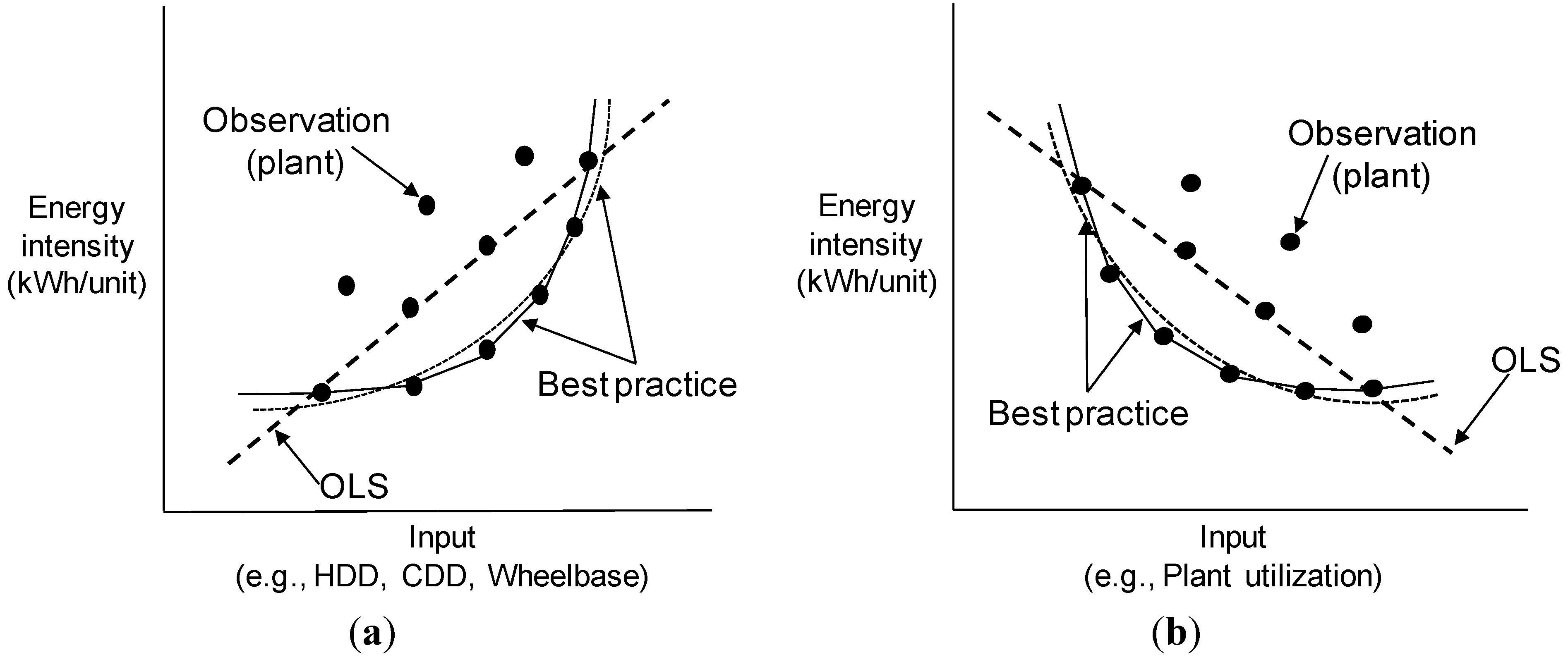
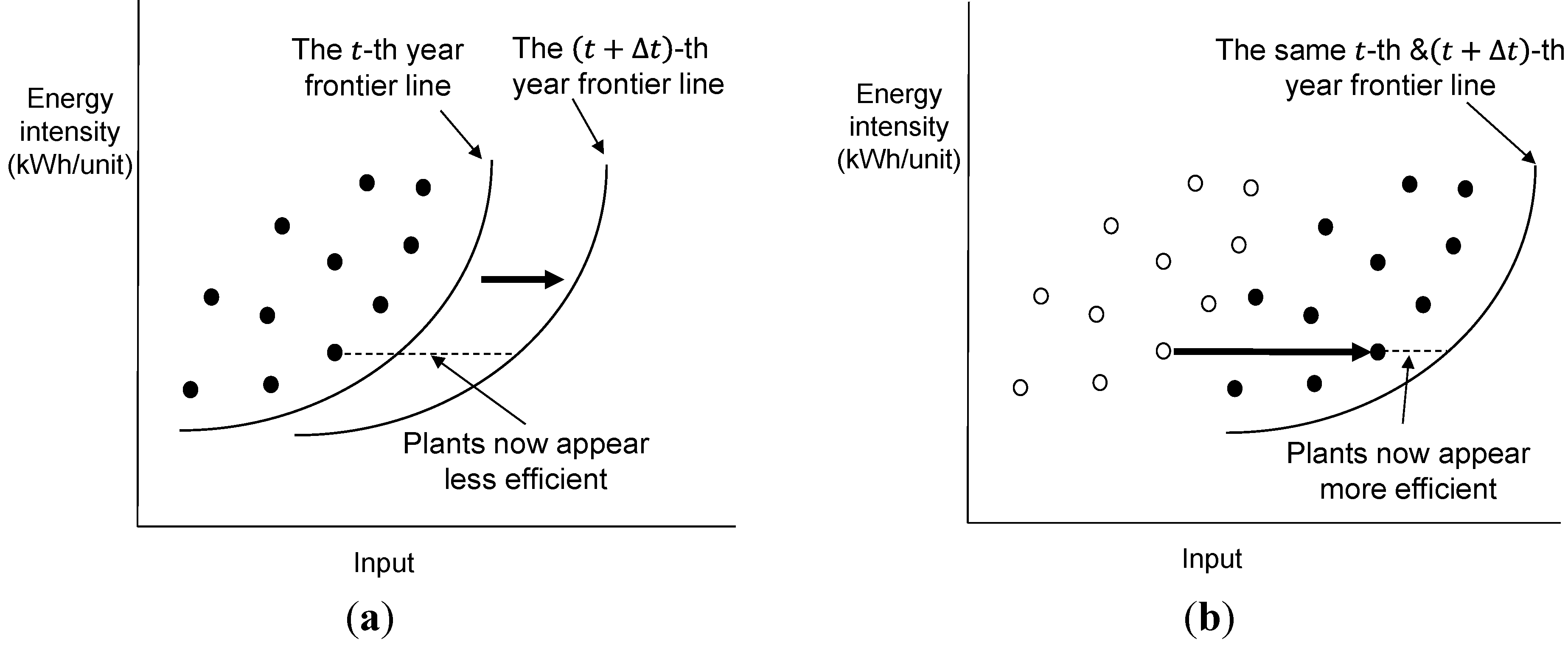
Figure 4 illustrates various relationships between energy intensity and non-energy factors (where the best practice indicates the lowest energy use achievable at the given operation conditions), with Figure 4a,b depicting a concave-up increasing energy intensity and a concave-up decreasing energy intensity, respectively. The concave-up increasing patterns may be observed when the energy intensity increases as the input variables (e.g., HDD, CDD, or wheelbase) increase, while the concave-up decreasing patterns may be observed when the input variables (e.g., plant utilization) have a negative relationship with the energy intensity.
Figure 4. Various relationships between energy intensity and non-energy factors (based on a cross-sectional data set). (a) Concave-up increasing energy intensity; (b) Concave-up decreasing energy intensity.
Energies 07 06196 g004
It is pertinent to observe that the plant energy efficiency at one point in time is subject to the impact of a structural technical improvement as follows:
  • The frontier line may shift independently of a set of observations where plants appear less efficient in the (t + ∆t)-th year than in the t-th year. This occurrence happens when a technical improvement is made in the industry (or company) during the time period between the t-th and the (t + ∆t)-th years, but the energy performances of target assessing plants remains unchanged and thus, the latter’s energy efficiency appears less efficient because the difference between the actual efficiency score and the best practice score increases. In the Malmquist literature, this occurrence is called technical change. Figure 5a depicts this case.
  • A set of observations may move independently closer to a frontier line while the frontier line remains unchanged during the period between the t-th and (t + ∆t)-th years. This occurrence happens when a technical improvement has not been made during the time period, but the target assessing plants have improved their energy performance during the same time period and, thus, their energy efficiency appears more efficient in the (t + ∆t)-th year than in the t-th year because the difference between the actual energy use and the best practice decreases. In the Malmquist literature, this occurrence is called efficiency change. Figure 5b depicts this case.
Aside from the two cases above, both a frontier line shift and a positive movement of a set of observations can happen simultaneously, in which case it may not be easy to differentiate the energy performance improvement of individual plants because the efficiency improvement of individual plants can be offset by the technical improvement of the industry. While SFA is likely to have trouble in distinguishing technical improvements from efficiency improvements, DEA can do so by implementing the Malmquist total factor productivity (TFP) index, which will be discussed in detail in Section 3.3.
This study uses Spearman’s rank-order correlation coefficient test to determine the consistency in ranks between SFA and DEA models in the illustrative study. The rationale for using this test is that though efficiency levels (or scores) differ between models, these methods may nonetheless generate similar rankings. If the two models’ rankings are completely different, then any action taken based on the assessment may be temporary and depend on which frontier model is employed.
Figure 5. Two main sources affecting changes in the plant energy efficiency over time. (a) Shifts in frontier line independent of a set of observations; (b) Movement of a set of observations closer to the frontier line.
Energies 07 06196 g005

3.1. Background of the Vehicle Assembly Process

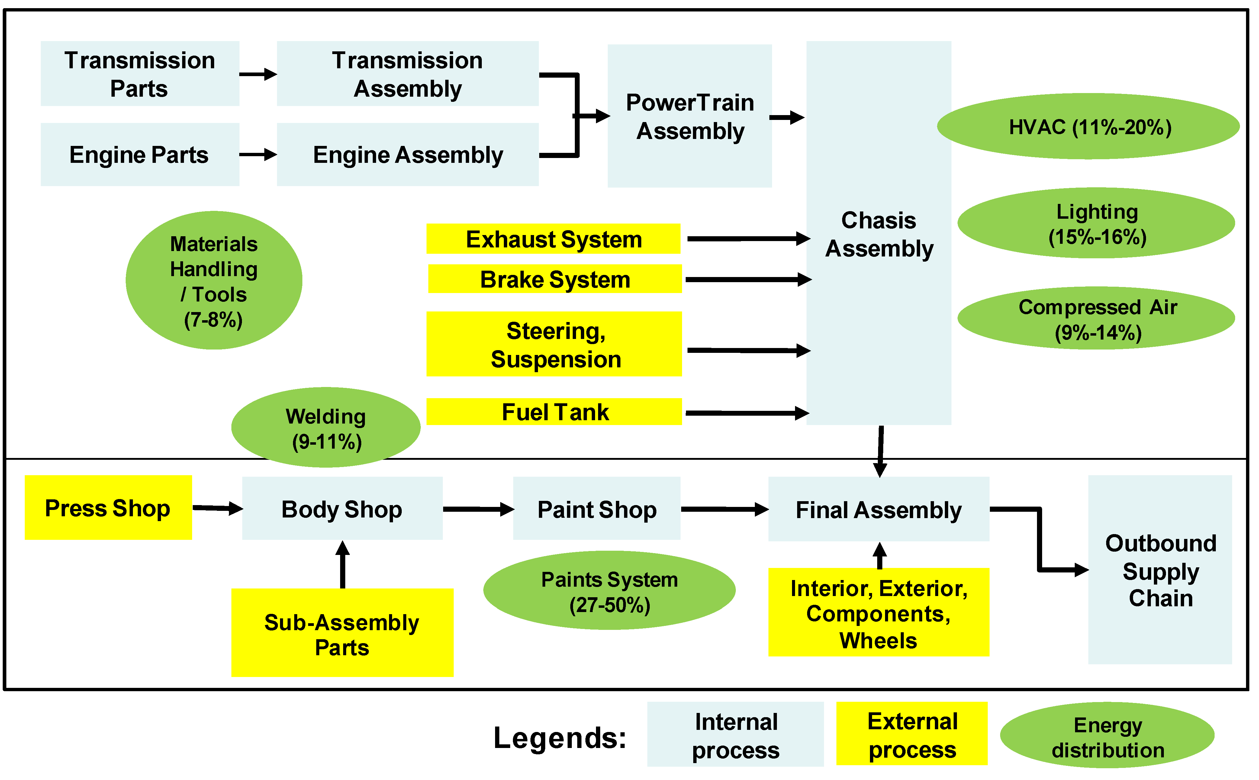
A typical automobile manufacturing process generally consists of three main processes: body shop, paint shop, and general assembly. The body shop transforms raw materials into the structure of the vehicle. Then, the paint shop applies a protective and visual coating to the product. Finally, the general assembly assembles all sub-components, such as the engine and seats, into the vehicle.
Two main types of energy utility used in a typical vehicle assembly plant are electricity and fuel (including natural gas). In general, fuel is used for direct heating or to generate steam that is considered as a secondary utility similar to compressed air in vehicle assembly plants. Steam is then used mainly in painting but is also utilized for space heating, car wash and other non-manufacturing activities. Electricity is the main energy source in vehicle assembly plants, and its main uses are painting, HVAC (heating, ventilation, and air conditioning), lighting, compressed air systems, and welding and materials handling/tools.
Figure 6 associates automotive manufacturing operations with the distribution of their energy use. Four identified largest energy-consuming operations are painting (27%–50%), HVAC and lighting (11%–20% and 15%–16%, respectively), and compressed air (9%–14%).
Figure 6. A typical vehicle assembly process and its energy distribution (modified from [21]).
Energies 07 06196 g006

3.2. Stochastic Frontier Analysis (SFA)

The SFA models in this study follow the model specification proposed by Battese and Coelli [15] and expands the cross-sectional data model specified by Boyd [10] to a panel data model by incorporating two cross-sectional data sets. The YEAR variable involved in the resultant SFA models accounts for a Hicksian neutral technological change model. Note that Hicksian models assume special parameters that may shift the frontier line due to structural change, such as the year of the observation. Although this concept does not sufficiently account for the balance between parameters, this paper uses the Hicksian neutral technical change concept because the balance between parameters is likely to remain unchanged for the time period until a technical improvement occurs. This stability occurs because the parameters used in this paper (e.g., HDD, CDD, wheelbase, utilization) are exogenous variables, thus effecting different operation conditions in different plants. This study developed two stochastic frontier models for electricity and fuel because they are the main energy utilities consumed in vehicle manufacturing plants (note: the background on the inclusion of each term in each model is discussed in Boyd [10]. For example, why are quadratic terms for HDD and CDD included in the electricity model and the quadratic term of plant utilization included in fuel model? Why is the wheelbase of a vehicle used as a control variable rather than some other variable(s) that may also reflect the vehicle size?). The proposed SFA model for electricity is:
E i Y i = A +   β 1 W B A S E i + β 2 H D D i +   β 3 H D D i 2 + β 4 C D D i +   β 5 C D D i 2 +   β 6 U t i l i +   β 7 Y e a r i +   u i v i
where:
  • E i : Total site electricity use at plant i in kWh;
  • Y i : Number of vehicles produced;
  • W B A S E i : Wheelbase (the distance between its front and rear wheels) of the largest vehicle produced in the plant in inch;
  • H D D i : Thousand heating degree days for the plant location and year;
  • H D D i 2 : H D D i squared;
  • C D D i : Thousand cooling degree days for the plant location and year;
  • C D D i 2 : C D D i squared;
  • U t i l i : Plant utilization rate, defined as output/capacity, where the denominator, capacity is a normalized capacity defined as equal to capacity line rate (or job per hour) × 235 working days × 16 working hours per day;
  • Y e a r i : t and t + t where t is the time period at which a significant technical improvement in energy efficiency is observed; and
  • β : Vector of parameters to be estimated.
Note that HDD is a metric for quantifying the amount of heating that buildings in a particular location require for a certain period (e.g., a specific month or year) such that HDD = n o . d a y s max ( 0.65   ( or   60 )   average day temperature ) . Similar to HDD, CDD is a metric for quantifying the amount of cooling that buildings in a particular location require for a certain period (e.g., a specific month or year) such that CDD = n o . d a y s max ( 0 , average day temperature 65   ( or   60 ) ) . Note that our study scales HDD and CDD by 1000. The variable v represents a measurement error to be distributed as a symmetric normal distribution, and N ( 0 , σ v 2 ) N ( 0 , σ v 2 ) and the variable u account for a technical inefficiency to be distributed as a half normal distribution, N + ( 0 , σ u 2 ) . Meanwhile, the proposed SFA model for fuel is:
F i Y i = A +   β 1 W B A S E i +   β 2 H D D i +   β 3 H D D i 2   + β 4 U t i l i +   β 5 U t i l i 2   +   β 6 Y e a r i +   u i v i
where, all the notations are specified identically to Equation (1) except that F i is the total site fuel use at plant i in 106 BTU. Note that this fuel model may not account for the real operation if the given plant uses steam-powered absorption chillers for air conditioning. Such chillers contribute more to the “fuel” load than the “electricity” load. If it is the case, CDD should be included in this model.
Equations (1) and (2) require several parameters to be solved, such as β , σ v 2 and σ u 2 . This paper uses the maximum likelihood method for parameter estimation and utilizes the parameterization of Battese and Corra [22], who replaced σ v 2 and σ u 2 with ε = u v , σ = σ u 2 + σ v 2 , λ = σ u 2 σ v 2 and γ = σ u 2 ( σ v 2 + σ u 2 ) . This parameterization is useful for calculating the maximum likelihood estimates because the parameter γ is now confined to exist between 0 and 1, a range that can be more easily searched to provide a good estimate in an iterative maximization process. The first step of the maximum likelihood method is defining the log-likelihood function of the model and the log of the density function for ε :
l o g φ ε ( ε ) = 1 2 l o g ( π 2 ) 1 2 l o g σ 2 + l o g Φ ( ελ σ 2 ) 1 2   ε 2 σ 2
with N independent observations, the log of the joint density function ε 1 , ,   ε N is:
l o g φ ( ε 1 , , ε N ) =   i = 1 N l o g φ ε ( ε i )   = 1 2 N   l o g ( π 2 ) 1 2 N   l o g   σ 2 + i = 1 N l o g Φ ( λε i σ 2 ) 1 2 σ 2 i = 1 N ε i 2
To emphasize that the error term ε depends on the parameter (vector) β , the log likelihood function can be expressed alternatively as:
l ( β , σ 2 , λ ) = 1 2 N   l o g ( π 2 ) 1 2 N   l o g σ 2 + i = 1 N l o g Φ ( λ ( y i f ( x i ; β ) ) σ 2 ) 1 2 σ 2   i = 1 N ( y i f ( x i ; β ) ) 2 .
The function l ( β , σ 2 , λ ) is the log-likelihood function, which depends on parameters to be estimated (in this cas β , σ 2 and λ ) and on the data ( x 1 , y 1 ), …, ( x N , y N ). The derivation of the log likelihood function is available in Bogetoft and Otto [23]. With σ 2 replaced with 1 N i = 1 N ( y i f ( x i ; β ) ) 2 , first-order partial derivatives for the function can be obtained.
First, the partial derivative of l ( β , λ ) with respect to β is:
β j l ( β , λ ) = λ σ i = 1 N ϕ ( λε i σ ) Φ ( λε i σ ) X j i + i = 1 N ε i X j i σ 2 ( 1 + λ N σ i = 1 N ϕ ( λε i σ ) Φ ( λε i σ ) ε i ) .
Second, the partial derivative of l ( β , λ ) with respect to λ is:
λ l ( β , λ ) = i = 1 N ϕ ( λ ϵ i σ ) Φ ( λ ϵ i σ ) ϵ i σ .
Coelli et al. [24] suggested a one-sided likelihood-ratio test to determine whether the variation in inefficiency ( u i ) is significant. The purpose of the test is to compare the parameter estimates in an ordinary least square regression model (OLS) with respect to the null-hypothesis, H 0 : γ = σ u 2 ( σ v 2 + σ u 2 ) = 0 , and the parameter estimates in SFA under the alternative hypothesis, H 1 : γ > 0 . The test value is calculated using Equation (3).
L R = 2 { l n [ L ( O L S ) L ( S F A ) ] } = 2 { l n [ L ( O L S ) ] l n [ L ( S F A ) ] }
where, L ( O L S ) and L ( O L S ) are the values of the likelihood function under OLS and SFA, respectively. In the illustrative study, this paper will calculate and compare the L R statistic with χ 1 2 α 2 ( 1 ) , then determine to accept or reject the null hypothesis. In other words, if the L R statistic exceeds α % critical value, we reject the null hypothesis of no inefficiency effects. If the null hypothesis H 0 : γ = 0 is accepted, it would indicate that σ u 2 is zero and hence that the inefficiency term u i should be removed from the model, thus, specifying parameters that can be consistently estimated using OLS.
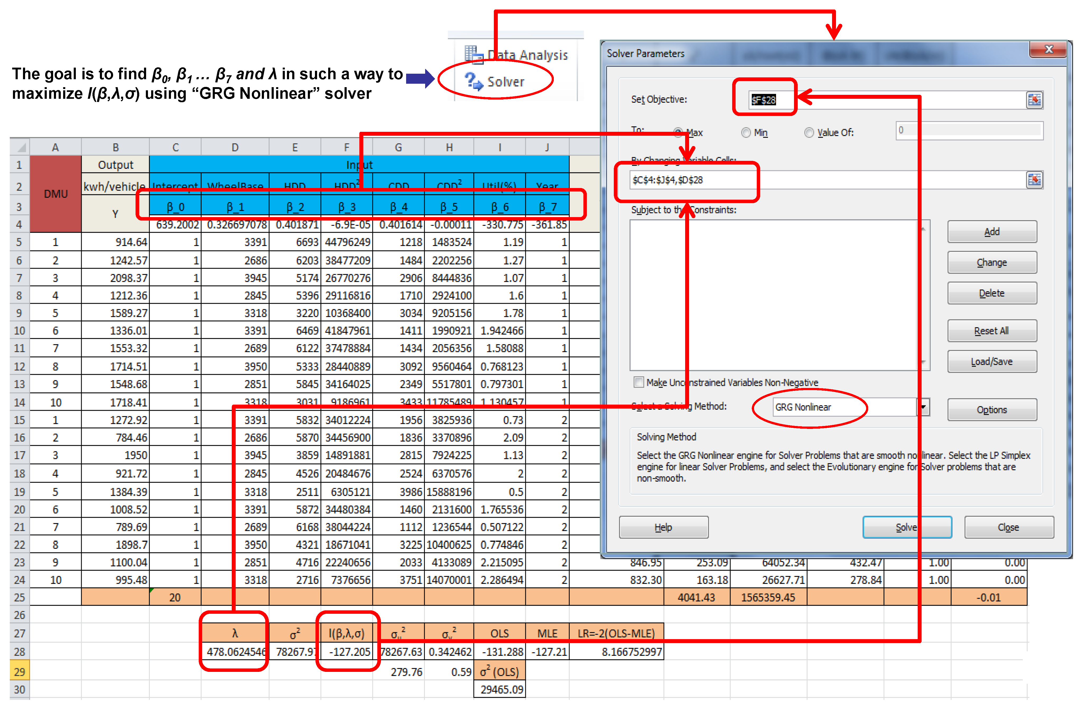
This study developed an Excel spreadsheet tool to obtain the maximum likelihood estimation of subset parameters in the aforementioned SFA models rapidly and intuitively. The tool can accommodate panel data, a half-normal inefficiency distribution and a normal measurement error distribution. Section 4 will show what the tool looks like. Regarding an energy performance indicator developed by a credential governmental organization, the U.S. Environmental Protection Agency (EPA) introduced energy performance indicators (EPIs) through its ENERGY STAR program to encourage a variety of U.S. industries to use energy more efficiently. One of the EPIs was developed for a plant-level energy performance indicator to benchmark manufacturing energy use in the automobile industry based on the SFA model [10]. Because a typical SFA model has a composite error term including symmetric (normal) measurement errors denoted by v i and one-sided (half-normal) inefficiencies denoted by u i , the frontier model takes the form of the following equation, as in Equations (1) and (2):
E i Y i = f ( X ; β ) + ε i
where, ε i = u i v i , v i ~   N ( 0 , σ v 2 ) and u i ~   N + ( 0 , σ u 2 ) . In addition, E i is the energy use of company i ; Y i is the measured production or service measured of company i ; X i is the economic decision variables (i.e., labor-hours worked, materials processed, plant capacity, or utilization rates) or external factors (i.e., heating and cooling energy loads); and β is the vector of parameters to be estimated statistically.
Given company data, Equation (4) can be expressed as Equation (5), thereby providing a way to compute the difference between the actual energy use and the predicted frontier energy use:
E i Y i f ( X ; β ) + v i = u i
Then, the EPI of company i is calculated from the probability distribution of u i as follows:
E P I = p r o b a b i l i t y ( e n e r g y   i n e f f i c i e n c y   E i Y i f ( X ; β ) + v i ) = 1 F ( E i Y i f ( X ; β ) + v i )
F ( ) is the cumulative probability density function of the appropriate one-sided density function for u i (e.g., gamma, exponential, truncated normal, and other functions). The value 1 F ( ) in Equation (6) defines the EPI score and may be interpreted as a percentile ranking of the company’s energy efficiency. However, in practice, the only measureable value is ui – vi = Ei/Yif(X;B). By implication, the EPI score 1 F ( u i v i ) is affected by the random component of v i , that is, the score will reflect the random influences that are not accounted for by the function   F ( ) . Because this ranking is based on the distribution of inefficiency for the entire industry, but normalized to the specific regression factors of the given company, this statistical model enables the user to answer the hypothetical but practical question, “How does my company compare to everyone else’s in my industry, if all other companies were similar to mine?”. This study will calculate the EPI scores of each plant based on the proposed SFA models in Section 4. Yee and Oh [25] used the EPI score as described in this section for selecting the optimal supply partner for composing semantic web services, when performance metrics for sustainable supply chain are important for automatic business composition, particularly at the service matchmaking phase.

3.3. Data Envelopment Analysis (DEA)

When a panel data set is available and one is interested in measuring the technical improvement in energy efficiency, the Malmquist total factor productivity (TFP) index can be used to reveal a positive or negative technical change across two distinct years such as t and t + t . One advantage of using the Malmquist TFP index is that it can be decomposed into a structural technical change (improvement or deterioration) and a technical efficiency change, where the structural technical change may account for the technical improvement (e.g., frontier line shifts between two distinct years), while the efficiency change indicates how well companies are improving to the frontier line. For example, when a frontier line shifts independently of the DMU set, DMUs appear less efficient, reflecting a positive technical change. By contrast, when a set of DMUs moves independently closer to the frontier line, DMUs appear more efficient, resulting in a positive technical efficiency change. If the frontier line shifts to a higher efficiency and simultaneously, a set of DMUs shifts to a higher efficiency, a positive TFP has occurred. Depending on the orientation used to measure the efficiency, (i.e., either output oriented or input oriented) the TFP indices differ. Recently, a new approach adopting a directional distance function was introduced to provide a flexibility in measurement by allowing negative input and output quantities. For more details on the underlying theory and application of directional distance function, see Nin et al. [26].
For the consistency between SFA and DEA models, a new vector variable Z i = ( HDD i , CDD i , Wheelbase i , 1 Utilization i ) is introduced to represent the systematic external factors given for i-th company or plant. Note that Z i takes the inverse of utilization because this study is based on the assumption of strong disposability where all the variables must have a non-decreasing relationship with the energy intensity. Then, our interest in defining the minimum energy intensity requirement to produce one unit of vehicle under the given external condition to i-th plant is expressed in the following function:
( E i Y i ) * = i n f { c a n   p r o c e s s   Z i   t o   p r o d u c e   o n e   u n i t   o f   v e h i c l e }
Equation (7) motivates the minimal energy density requirement in terms of micro-economic concept. It is possible to connect this motivation expressed in Equation (7) with the interpretation of input distance function that we need to calculate TFP indices. For more specific details of the theoretical development on this connection, see Boyd [27]. An input oriented distance function corresponding to Equation (7) is as follows:
D I ( Z i , E i Y i ) = s u p { : ( E i Y i ) c a n   p r o c e s s   Z i   t o   p r o d u c e   o n e   u n i t   o f   v e h i c l e }
Since a distance function is defined, it is possible to calculate the TFP index. In our context, the TFP index requires four distance function values, specifically, D I t ( Z t , E t Y   t ) , D I t + t ( Z t , E t Y   t ) , D I t ( Z t + t , E t + t Y   t + t ) , and D I t + t ( Z t + t , E t + t Y   t + t ) , where the notation D I t ( Z t + t , E t + t Y   t + t ) represents the distance from the period t + t observation to the period t technology. Vector forms, Z t and E t Y   t represent ( Z 1 t ,   Z 2 t ,   ,   Z N t ) and ( E 1 t Y   1 t , E 2 t Y   2 t ,   , E N t Y   N t ) , respectively. The subscript “I” has been introduced to remind that this is an input -orientated measures.
Note that each distance function has an equivalent DEA model. For example, D I t ( Z t , E t Y   t ) is identical to the following DEA model:
D I t ( Z t , E t Y   t ) = min ϕ , λ ϕ s . t . Z i t + Z t λ 0 , ϕ ( E i t Y i t ) + ( E t Y   t ) λ 0 λ 0
The remaining three DEA models are simple variants of this form. Table 3 summarizes all the forms.
Table 3. DEA models required to calculate Malmquist TFP indices.
Input Oriented Envelopment Forms
D I t + t ( E t + t Y t + t , Z t + t ) =   min ϕ , λ   ϕ , s . t .   Z i t + t + Z t + t λ 0 , ϕ ( E i t + t Y i t + t ) + E t + t Y t + t λ 0 , λ 0
(10)
D I t ( E t + t Y t + t , Z t + t ) =   min ϕ , λ   ϕ , s . t .   Z i t + t + Z t λ 0 , ϕ ( E i t + t Y i t + t ) + E t Y t λ 0 , λ 0
(11)
D I t + t ( Z t , E t Y t ) =   min ϕ , λ ϕ , s . t .   Z i t + Z t + t λ 0 , ϕ ( E i t Y i t ) + E t + t Y t + t λ 0 , λ 0
(12)
LP (Linear Program) (9) is used to calculate the efficiency of the t -th time period relative to t -th time period technology, while LP (10) is used to calculate the efficiency of ( t + t ) -th time period relative to ( t + t ) -th time period technology. Similarly, LP (11) is used to calculate the efficiency of the ( t + t ) -th time period relative to t -th time period technology, while LP (12) is used to calculate the efficiency of the t -th time period relative to ( t + t ) -th time period technology.
Once D I t ( Z t , E t Y   t ) , D I t + t ( Z t , E t Y   t ) , D I t ( Z t + t , E t + t Y   t + t ) , and D I t + t ( Z t + t , E t + t Y   t + t ) are obtained, the Malmquist TFP index can be calculated and then rearranged such that it is equivalent to the product of a technical efficiency change index and an index of technical change.
m I ( Z t + t , E t + t Y   t + t , Z t , E t Y   t ) = [ D I t ( Z t + t , E t + t Y   t + t ) D I t ( Z t , E t Y   t ) × D I t + t ( Z t + t , E t + t Y   t + t ) D I t + t ( Z t , E t Y   t ) ] 1 / 2 = D I t + t ( Z t + t , E t + t Y   t + t ) D I t ( Z t , E t Y   t ) [ D I t ( Z t + t , E t + t Y   t + t ) D I t + t ( Z t + t , E t + t Y   t + t )   × D I t ( Z t , E t Y   t ) D I t ( Z t , E t Y   t ) ] 1 / 2
The first and second term of Equation (13) correspond to an efficiency change and a structural technical change, respectively, as follows:
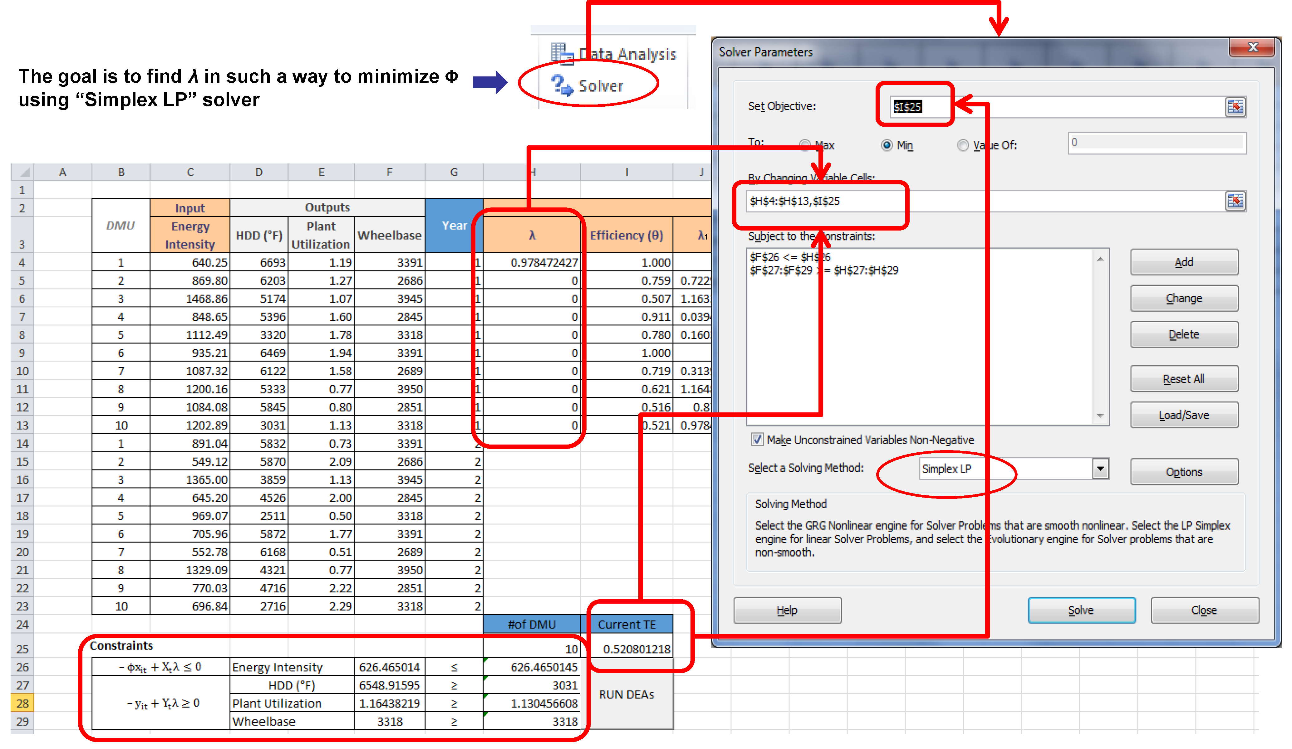
E f f i c i e n c y   c h a n g e =   D I t + t ( Z t + t , E t + t Y   t + t ) D I t ( Z t , E t Y   t )
Meanwhile,
T e c h n i c a l   c h a n g e =   [ D I t ( Z t + t , E t + t Y   t + t ) D I t + t ( Z t + t , E t + t Y   t + t )   × D I t ( Z t , E t Y   t ) D I t + t ( Z t , E t Y   t ) ] 1 / 2
Note that the ϕ and λ are likely to assume different values in the four DEA models in Table 3. Furthermore, these four models must be calculated for each plant in the sample. Thus, if there are 10 plants and two time periods, then 40 linear programing problems must be solved. To streamline this multiple calculation procedure, this study developed an Excel spreadsheet tool as does for the SFA models. The developed tool uses VBA in Excel and automates iterations for solving multiple linear programing models. Section 4 will show what the tool looks like.

4. Illustrative Study

This paper uses artificial data sets for illustrative studies because of intellectual property issues. The data sets were generated to resemble real-world data as close as possible. Although SFA and DEA are generally conducted with real industry data to suggest new insights or interesting finds, the authors believe that the use of artificial data sets will not be detrimental to the overall purpose of this study that is to demonstrate the benchmarking process from building frontier models to identifying any structural technical improvement. The generated artificial data sets are listed in Table 4 in which two different years’ data (years t and t + ∆t) for 10 vehicle assembly plants are considered. Regarding the scope of assembly plant, the authors are only considering body shop, paint shop and GA. In fact, these areas vary widely in terms of work volume, labor hours or energy usage depending on their level of in-house versus outsourced tasks. The data are generated with an in-house case assumed. In addition, the authors assumed that the major energy-consuming operations are similar among plants. For example, plants are assumed to use electricity-powered chiller, solvent-borne paint system, gas-fired direct heating system, and air conditioning in place.
Table 4. Plant data used in the illustrative studies.
Plantt-th Yeart + ∆t-th Year
Wheel Base (inch)HDD (1000)CDD (1000)UtilElectricity Intensity (kWh/Unit)Fuel Intensity (106 BTU/Unit)Wheel Base (inch)HDD (1000)CDD (1000)UtilElectricity Intensity (kWh/Unit)Fuel Intensity (106 BTU/Unit)
1133.506.691.221.19914.642.18133.505.831.960.731272.923.04
2105.756.201.481.271242.572.97105.755.871.842.09784.461.87
3155.325.172.911.072098.375.01155.323.862.821.1319504.66
4112.015.401.711.601212.362.90112.014.532.522.00921.722.20
5130.633.223.031.781589.273.80130.632.513.990.501384.393.31
6133.506.471.411.941336.013.19133.505.871.461.771008.522.41
7105.876.121.431.581553.323.71105.876.171.110.51789.691.89
8155.515.333.090.771714.514.10155.514.323.230.771898.74.54
9112.245.852.350.801548.683.70112.244.722.032.221100.042.63
10130.633.033.431.131718.414.10130.632.723.752.29995.482.38
This study uses a commercially available spreadsheet package, Excel, to build the SFA and DEA models. Excel provides an add-on tool called Solver with different solving method options such as Simplex or GRG (Generalized Reduced Gradient). Using the GRG solver method facilitates the maximum likelihood estimation of subset parameters of the proposed SFA models. The example in Figure 7 illustrates a case in which the tool accommodates plant-level input panel data on electricity and builds a model corresponding to Equation (1), thus, estimating parameters for the half-normal inefficiency distribution and the normal measurement error distribution.
Figure 7. SFA model estimation using MS-Excel Solver with “GRG Nonlinear” selected.
Energies 07 06196 g007
The estimated parameters for the electricity and fuel SFA models are shown in Table 5 where β 6 and β 7 are the coefficient representing YEAR in the fuel SFA model and in the electricity SFA model, respectively. The one-sided likelihood-ratio test values (LR) for both models reveal that the models are adequate at the 99.5% significance level and that the models have very little error attributable to random noise, with most departures attributable to inefficiency. Therefore, the null-hypothesis, H 0 : γ = σ u 2 ( σ v 2 + σ u 2 ) = 0 , is rejected, and the alternative hypothesis H 1 : γ > 0 with technical inefficiency effect is accepted for both the electricity and fuel SFA models. This statistical results show that a structural technical improvement in electricity ( β 7 of the electricity SFA model) and fuel ( β 6 of the fuel SFA model) occurred during the period. Furthermore, β 7 and β 6 are statistically significant at the 90% level (−1.91 < t0.95 (12) = −1.782) and the 85% level ( t 0.95 ( 13 ) = 1.771 < −1.6 < t0.9 (13) = −1.350) in a two-tailed test, respectively. These results indicate that, all other factors being equal, an average reduction of 330.77 (kWh) and 253.55 (kWh) in the electricity and fuel per vehicle has occurred, leading to efficiency gains of $41.73/vehicle (note: the calculation assumes $0.1/kWh for electricity and $0.03413/kWh (=0.03413 therm/kWh × $1/therm) for natural gas). This magnitude of efficiency gains may seem small in the unit cost of production but may offer considerable energy cost savings and significantly reduce the environmental impact when the total production is considered. For example, let us assume that a car manufacturing company produces nine million cars per year and must solely purchase CO2 credits from a market to emit CO2. Given these condition, if the company achieved the aforementioned magnitude of efficiency gains, then the total cost savings from energy reduction and a reduced environment impact would be $428 M (note: $428 M ≈ 9,000,000 × [$41.73 + (330.77 kWh + 253.55 kWh)/1000 × $10]; the CO2 credit price in the market is assumed to be $10 per CO2 ton). ENERGY STAR® plant energy performance indicator (EPI) values are also calculated, and the results are summarized in Table A1.
Table 5. Parameter estimates for the SFA models (Notations for significance level in a two-tailed test: *** (99%); ** (90%); * (85%)).
VariablesEstimates for the Electricity SFA Model (Standard Error; t-Ratio)Estimates for the Fuel SFA Model (Standard Error; t-Ratio)
β0650.490.67
β18.22 (6.05; 1.36)0.02 (0.00; 10.15) ***
β2394.87 (1159.16, 0.34)1.53 (1.38; 1.11)
β3−68.34 (123.01; −0.56)−0.21 (0.15; −1.40)
β4410.22 (1297.51; 0.32)−0.21 (2.83; −0.07)
β5−107.80 (268.42; −0.4)−0.16 (1.03; −0.16)
β6−331.85 (173.66; −1.91) **−0.86 (0.53; −1.60) *
β7−361.87 (191.46; −1.89) **NA
σu279.790.68
σv0.550.00
λ = σ u σ v
505.96614.92
L(OLS)−131.28−10.29
L(SFA)−127.21−6.81
LR8.17 > χ 1 2 × 0.005 2 ( 1 ) = 6.6356.97 > χ 1 2 × 0.005 2 ( 1 ) = 6.635
Using the Simplex solver, this study developed a spreadsheet tool for DEA, too. The developed tool uses VBA in Excel and automates iterations for solving multiple linear programing models. Briefly, with respect to automation logic, the tool uses “For” loop to automate iterations of solving multiple linear programing models in which the Solver with the “Simplex” optimization option calculates the efficiency for each DMU and the results are recorded in a table using the copy/paste function (note: the three major functions used in the loop statement of the VBA programing are as follows: (1) “SolverOk”—defines the objective function and the decision variables; (2) “SolverAdd”—defines model constraints; and (3) “SolverSolv”—runs Solver). Figure 8 illustrates an example in which the tool accommodates plant-level input panel data on fuel corresponding to LP (7). Table 6 and Table 7 present the Malmquist indices obtained by solving the DEA models for electricity and fuel, respectively. Three indices are presented for each firm, such as efficiency change (relative to a CRS technology), technical change, and total factor productivity change. It should be noted that the technical change of each model from t to t + t increases (greater than 100%), indicating that there has been a structural technical improvement in energy performance over the years. The DEA efficiency at each year is also calculated and summarized in Table A2 and Table A3.
Figure 8. DEA model implementation using MS-Excel Solver with “Simplex LP”.
Energies 07 06196 g008
Table 6. Malmquist index summary (Electricity).
DMUEfficiency ChangeTechnical ChangeTotal Factor Productivity Change
178%106%82%
2123%155%190%
377%138%106%
492%166%152%
576%175%133%
698%131%128%
7135%124%166%
862%147%91%
985%172%147%
10100%187%187%
Mean92%149%139%
Table 7. Malmquist index summary (Natural Gas).
DMUEfficiency ChangeTechnical ChangeTotal Factor Productivity Change
178%92%72%
2132%146%192%
3117%92%108%
499%148%146%
590%109%98%
698%129%127%
7139%122%169%
898%92%90%
9147%132%194%
10187%122%229%
Mean113%121%143%
It makes sense to compare the estimated parameters to those of existing estimated models in terms of value and sign as part of cross-validation if there have been similar estimation works. The 2000 and 2005 models elicited by Gale Boyd [28] have the identical model configuration with this study. Therefore, a comparison on the estimated parameters was conducted between those models and the results are summarized in Table B1 and Table B2 in Appendix B. One challenge against the comparison was that the datasets of two models are significantly different. The 2000 and 2005 models were based on real data composed by collecting some sample plant data from major car making companies in U.S. while this study generated an artificial dataset by simulating a population that resembles GM plants located in a specific region. Due to the large difference between datasets, the differences in magnitude between parameter values exist. However, the orders of magnitude between parameter values are in the same range and the directions of relationships between systematic external factors and energy intensity (i.e., signs of estimated parameters) turned out consistent. The authors again want to clarify that the datasets used in this study are simulated and should not be taken to be applicable to the industry, but are only illustrative of the proposed models.
In order to measure the consistency between the SFA and the DEA approaches on the efficiency ranking results for firms, a Spearman’s rank correlation coefficient test was conducted. Spearman’s rank correlation coefficient values are 0.9 and 0.25 for t and t + t , respectively, in electricity, and 0.3 and 0.38 for t and t + t , respectively, in natural gas. All of the rank correlation coefficient values are positive, indicating that the ranks of the SFA and DEA results have moderate (in t ) and small (in t + t ) positive linear relationships.
It seems that it would be more useful to compare best practices with inefficient practices to identify energy reduction opportunities after computing numerical efficiencies and locating the best and inefficient performance plants. Finding energy reduction opportunities must be preceded by understanding high energy cost drivers for inefficient plants. For this purpose, Oh and Hildreth [12], Jurek et al. [29], and Oh et al. [30] proposed activity-based decision steps including a step of comparing hourly average energy use of each activity between best practice plants and less efficient plants followed by figuring out which activity are problematic cost drivers for less efficient plants.

5. Conclusions

This paper proposes a benchmarking process using stochastic and deterministic frontier analysis models, specifically, SFA and DEA, to identify industry-wide or company-wide structural technical improvement in energy efficiency with a focus on the car manufacturing industry. The quantitative identification of technical improvement in energy efficiency is important to help car manufacturing companies evaluate the effectiveness of the various energy efficiency programs that they may have implemented, in many cases supported by government R&D or financial programs. This paper proposed SFA models that incorporate the Hicksian neutral technological change concept and DEA models implemented to calculate Malmquist Productivity Change indices. Illustrative examples of the proposed models are presented to demonstrate the overall benchmarking process to find frontier lines and to measure the shifts of the frontier line that were used to proxy the structural technical improvement in energy efficiency. A log likelihood ratio test and a Spearman rank-order correlation coefficient test were conducted to test the significance of the SFA model and its consistency with the DEA model, respectively. ENERGY STAR® plant energy performance indicator values were also calculated. The results of the analysis based on the SFA models calculated total efficiency gains of $41.73/vehicle during the tested period. The tools developed for illustrative examples are available upon request at authors.
Regarding future work, one priority is to enhance the proposed SFA and DEA models to enable them to account for structural technological change by including the time-varying behavior of the inefficiency effects, thereby identifying more extensive factors affecting the technical change. Additionally, the authors are interested to extend this research to implement a directional distance function in calculating the Malmquist TFP indices. Since the paper just covered automotive manufacturing energy consumption in the context of other industries, the authors want to further study the energy consumption in an automotive life cycle. Recently, an automotive life cycle analysis (e.g., GM’s carbon footprint) reveals that the supply chain for automotive parts is ten times more energy intensive than OEM’s operations. This demonstrates that extending energy efficiency methods into the automotive part supply chain can contribute a major reduction in car making industry carbon footprint. Therefore, there is an opportunity to extend the proposed SFA and DEA models to automotive part supply chain as a possible future work.

Author Contributions

The presented work is a product of the intellectual environment of the whole team. All members have contributed in various degrees to the analytical methods used, to the tool development, and to the illustrative example design and implementation.

Appendix A. SFA and DEA Results

Table A1. SFA results in terms of EPI.
DMUt-th Year(t + ∆t)-th Year
ElectricityNGElectricityNG
1100%100%66%42%
226%31%24%28%
316%16%26%14%
498%100%100%100%
599%86%81%100%
66%6%40%40%
71%2%99%92%
899%100%26%24%
935%30%37%31%
1093%96%56%83%
Mean57%57%56%55%
Note that DMUs 6 and 7 show the lower efficiency in Table B1 in t-th Year. These low efficiencies are caused by the large difference between their average practices and best practices. These results, however, also indicate that DMUs 6 and 7 have higher potentials to further improvement in energy savings.
Table A2. DEA results (Electricity).
DMU d 0 t ( x t , y t ) d 0 t + t ( x t , y t ) d 0 t ( x t + t , y t + t ) d 0 t + t ( x t + t , y t + t )
1100%108%94%78%
282%65%192%100%
377%55%81%59%
4100%69%173%92%
5100%62%144%76%
6100%74%125%98%
774%52%107%100%
899%68%91%61%
989%58%146%76%
10100%58%202%100%
Mean92%67%135%84%
Table A3. DEA results (Natural Gas).
DMU d 0 t ( x t , y t ) d 0 t + t ( x t , y t ) d 0 t ( x t + t , y t + t ) d 0 t + t ( x t + t , y t + t )
1100%109%72%78%
276%65%183%100%
351%55%55%59%
491%69%149%90%
578%61%65%70%
6100%75%123%98%
772%52%107%100%
862%67%56%61%
952%54%138%76%
1052%56%158%97%
Mean73%66%111%83%

Appendix B. Comparison of Estimated SFA Parameters

Table B1. Comparison of electricity SFA model parameters.
ParameterThis Study (Based on Simulated Data)2000 Model [28]2005 Model [28]Direction of the Relationship
Constant650.49369.39−91.84N/A
Wbase8.222.772.03
HDD394.87−48.41163.06
HDD2−68.344.79−15.17
Util−331.85−138.61−112.54
CDD410.22−59.32−223.89
CDD2−107.8041.9186.61
Table B2. Comparison of fuel SFA model parameters.
ParameterThis Study (Based on Simulated Data)2000 Model [28]2005 Model [28]Direction of the Relationship
Constant0.673.827−0.526N/A
Wbase0.020.003220.019
HDD1.53−0.5450.439
HDD2−0.210.11
Util−0.21−6.788−0.072
Util2−0.162.399

Conflicts of Interest

The authors declare no conflict of interest.

References

  1. Annual Energy Review 2011. Available online: http://www.eia.gov/totalenergy/data/annual/pdf/aer.pdf (accessed on 22 September 2014).
  2. 2011 Annual Survey of Manufacturers (ASM). Available online: https://www.census.gov/manufacturing/asm (accessed on 22 September 2014).
  3. 2012 GM Sustainability Report. Available online: http://www.gmsustainability.com (accessed on 22 September 2014).
  4. 2012 Volkswagen Sustainability Report. Available online: http://nachhaltigkeitsbericht2012.volkswagenag.com/en.html (accessed on 22 September 2014).
  5. 2012 Ford Sustainability Report. Available online: http://corporate.ford.com/microsites/sustainability-report-2012-13/default (accessed on 22 September 2014).
  6. 2012 BMW Sustainability Report. Available online: http://www.bmwgroup.com/e/0_0_www_bmwgroup_com/verantwortung/svr_2012/index.html (accessed on 22 September 2014).
  7. 2012 Toyota North American Environmental Report. Available online: http://www.toyota.com/about/environmentreport2012/eco-efficient.html (accessed on 22 September 2014).
  8. Lin, L.-C.; Tseng, L.-A. Application of DEA and SFA on the measurement of operating efficiencies for 27 international container ports. In Proceedings of the Eastern Asia Society for Transportation Studies, Bangkok, Thailand, 21–24 September 2005; Volume 5, pp. 592–607.
  9. Galitsky, C.; Worrell, E. Energy Efficiency Improvement and Cost Saving Opportunities for the Vehicle Assembly Industry; Lawrence Berkley National Laboratory (LBNL): Orlando, FL, USA, 2008. [Google Scholar]
  10. Boyd, G.A. Development of a Performance-Based Industrial Energy Efficiency Indicator for Automobile Assembly Plants; Technical Report ANL/DIS-05-3; Argonne National Laboratory: DuPage County, IL, USA, 2005. [Google Scholar]
  11. Sullivan, J.L.; Burnham, A.; Wang, M.Q. Energy and Carbon Emissions Analysis of Vehicle Manufacturing and Assembly; Technical Report ANL/ESD 10–6; Argonne National Laboratory: DuPage County, IL, USA, 2010. [Google Scholar]
  12. Oh, S.-C.; Hidreth, A.J. Decisions on energy demand response option contracts in smart grids based on activity-based costing and stochastic programming. Energies 2013, 6, 425–443. [Google Scholar]
  13. Aigner, D.J.; Lovell, C.A.K.; Schmidt, P. Formulation and estimation of stochastic frontier production function models. J. Econ. 1977, 6, 21–37. [Google Scholar]
  14. Meeusen, W.; van den Breoek, J. Efficiency estimation from Cobb-Douglas production functions with composed error. Int. Econ. Rev. 1977, 18, 435–444. [Google Scholar]
  15. Battese, G.E.; Coelli, T.J. A model for technical inefficiency effects in a stochastic frontier production function for panel data. Empir. Econ. 1995, 20, 325–332. [Google Scholar]
  16. Charnes, A.; Cooper, W.W.; Rhodes, E. Measuring the efficiency of decision making unit. Eur. J. Oper. Res. 1978, 2, 429–444. [Google Scholar]
  17. Banker, R.D.; Charnes, A.; Cooper, W.W. Some models for estimating technical and scale inefficiencies in data envelopment analysis. Manag. Sci. 1984, 30, 1078–1092. [Google Scholar]
  18. Färe, R.; Grosskopt, S.; Margaritis, D. Malmquist productivity indexes and DEA. In Handbook of Data Envelopment Analysis, 2nd ed.; Cooper, W.W., Seiford, L.M., Zhe, J., Eds.; Springer: Berlin, Germany, 2011; Volume 164, pp. 127–149. [Google Scholar]
  19. Productivity Commission. Electricity Network Regulatory Frameworks; Inquiry Report, 1(62); Australian Government, Productivity Commission: Melbourne, Australia, 2013. [Google Scholar]
  20. The Nonparametric Approach in Efficiency Analysis: Recent Developments and Applications. Available online: http://www.siepi.univpm.it/sites/www.siepi.univpm.it/files/siepi/SIEPI%202012/papers/Daraio.pdf (accessed on 22 September 2014).
  21. US Department of Energy. Technology Roadmap for Energy Reduction in Automotive Manufacturing; Office of Energy Efficiency & Renewable Energy, Industrial Technologies Program and U.S. Council for Automotive Research: Washington, DC, USA, 2008.
  22. Battese, G.E.; Corra, G.S. Estimation of a production frontier model: With application to the pastoral zone of eastern Australia. Aust. J. Agric. Econ. 1977, 21, 169–179. [Google Scholar]
  23. Bogetoft, P.; Otto, L. Benchmarking with DEA, SFA, and R; Springer: Berlin, Germany, 2011. [Google Scholar]
  24. Coelli, T.S.; Prasada Rao, D.S.; O’Donnell, C.J.; Battese, G.E. An Introduction to Efficiency and Productivity Analysis, 2nd ed.; Springer: Berlin, Germany, 2005. [Google Scholar]
  25. Yee, J.T.; Oh, S.-C. Technology Integration to Business; Springer: Berlin, Germany, 2012. [Google Scholar]
  26. Nin, A.; Arndt, C.; Hertel, T.W.; Preckel, P.V. Bridging the gap between partial and total factor productivity measures using directional distance functions. Am. J. Agric. Econ. 2003, 85, 928–942. [Google Scholar]
  27. Boyd, G.A. Estimating plant level energy efficiency with a stochastic frontier. Energy J. 2008, 29, 23–43. [Google Scholar]
  28. Boyd, G.A. Estimating the changes in the distribution of energy efficiency in the U.S. automobile assembly industry. Energy Econ. 2014, 42, 81–87. [Google Scholar]
  29. Jurek, P.; Bras, B.; Guldberg, T.; D’Arcy, J.B.; Oh, S.-C.; Biller, S.R. ABC applied to automotive manufacturing. In Proceedings of the IEEE Power & Energy Society General Meeting, San Diego, CA, USA, 22–26 July 2012.
  30. Oh, S.-C.; D’Arcy, J.B.; Arinez, J.F.; Biller, S.R.; Hidreth, A.J. Assessment of energy demand response options in smart grid utilizing the stochastic programming approach. In Proceedings of the IEEE Power & Energy Society General Meeting, Detroit, MI, USA, 24–28 July 2011.

