Article

Effect of Various Excitation Conditions on Vibrational Energy in a Multi-Degree-of-Freedom Torsional System with Piecewise-Type Nonlinearities

1
Division of Mechanical and Automotive Engineering, Kongju National University, Cheonan-si, Chungcheongnam-do 314-701, Korea
2
School of Mechanical Engineering, Yeungnam University, Gyeongsan-si, Gyeongsangbuk-do 712-749, Korea
*
Author to whom correspondence should be addressed.
Energies 2015, 8(10), 10861-10882; https://doi.org/10.3390/en81010861
Submission received: 31 August 2015 / Revised: 22 September 2015 / Accepted: 23 September 2015 / Published: 29 September 2015
(This article belongs to the Collection Wind Turbines)

Abstract

:
Dynamic behaviors in practical driveline systems for wind turbines or vehicles are inherently affected by multiple nonlinearities such as piecewise-type torsional springs. However, various excitation conditions with different levels of magnitudes also show strong relationships to the dynamic behaviors when system responses are examined in both frequency and time domains. This study investigated the nonlinear responses of torsional systems under various excitations by using the harmonic balance method and numerical analysis. In order to understand the effect of piecewise-type nonlinearities on vibrational energy with different excitations, the nonlinear responses were investigated with various comparisons. First, two different jumping phenomena with frequency up- and down-sweeping conditions were determined under severe excitation levels. Second, practical system analysis using the phase plane and Poincaré map was conducted in various ways. When the system responses were composed of quasi-periodic components, Poincaré map analysis clearly revealed the nonlinear dynamic characteristics and thus it is suggested to investigate complicated nonlinear dynamic responses in practical driveline systems.

1. Introduction

Practical driveline components in various mechanical systems such as wind turbines and vehicles inherently contain various nonlinearities, such as multi-staged clutch dampers, gear backlashes, and drag torques [1,2,3]. Unloaded gears of typical gearboxes, excited by the dynamic torque from the engine fluctuation with even small mean loads, induce vibro-impacts due to gear backlash and multi-staged clutch damper. This phenomenon is associated with the NVH performance (vibration and noise) of the target system and is highly nonlinear behavior, and difficult to analyze. In order to investigate nonlinear dynamic responses in a simple mechanical system, many studies have been conducted using the harmonic balance method (HBM) [4,5,6,7,8,9,10,11,12]. For example, Peng et al. [4] suggested nonlinear output frequency response functions using the Duffing oscillator to simulate strong nonlinear equations. Al-shyyab and Kahraman [5] investigated sub-harmonics and chaotic motions in a multi-mesh gear train using a nonlinear time-varying dynamic model. Chen et al. [6] used the incremental harmonic balance (IHB) method to investigate the limit cycle oscillation of a two-dimensional airfoil with parameter variability in an incompressible flow. Genesio and Tesi [7] presented two practical methods to predict the existence and the location of chaotic motions. Masiani et al. [8] examined the system responses under a hysteretic restoring force by employing two degree-of-freedom (DOF) chain systems given sinusoidal input. Raghothama and Narayanan [9] used the incremental harmonic balance method to obtain the periodic motions of a 3DOF nonlinear model of a geared rotor system subjected to parametric excitation under sinusoidal excitation. Raghothama and Narayanan [10] investigated the bifurcation of an articulated loading platform given harmonic excitation. Shen et al. [11] studied the dynamic behaviors of a spur gear pair by employing the incremental harmonic balance method. Wong et al. [12] presented the nonlinearities in the restoring force by employing the incremental harmonic balance method.
Prior research has mostly focused on the component levels or local areas as a part of integrated systems. Thus, this study investigated the nonlinear effects under various excitation conditions at the combined physical system level. The macro-system such as driveline in the wind turbine is much related to durability problems under the dynamic conditions. In order to expect the failure of the dynamic conditions, the transmission errors including various types of gear nonlinearities should be considered. Regarding this issue, theoretical background and simulation models can be directly connected to each other. In order to examine the nonlinear dynamic behaviors, a three DOF system model reduced from the original system shown in Figure 1 will be used [1,2,3]. Piecewise-type nonlinearities such as multi-staged clutch dampers will be employed to simulate the nonlinear dynamic behaviors in terms of relative motions in a simple driveline system model. The large body of literature for piecewise-type nonlinearities and other problems can be reviewed [13,14,15,16,17,18,19,20,21,22,23].
This study considers the asymmetrical piecewise-type nonlinearities based on the combined level of a driveline system [1,2,3,24]. The main objectives of this study are: (1) investigate the trends of nonlinear dynamic responses under various engine excitation conditions, which will lead to understanding of the relationship of nonlinear dynamic behaviors with different excitation levels by advancing prior studies [1,2,3,16,24]. (2) Poincaré map models for practical systems are suggested. Nonlinear responses with different excitation conditions were clearly observed with multiple comparisons. (3) quasi-periodic responses in the unstable response regimes in a practical system will be examined using HBM and numerical simulation (NS). Particularly, the nonlinear dynamic characteristics in the phase planes and Poincaré maps will be clearly determined by comparing the stable ranges with the unstable ones in the frequency domain. No efforts have been devoted to the simulation of nonlinear vibrational energy effects with practical parameter values obtained from experiments. In addition, no prior studies have systematically investigated the dynamic responses of the driveline system with respect to various types and levels of excitation conditions, and compared the results using HBM and numerical simulation. The simplest model is developed, with only necessary elements for describing the vibrational behavior remaining, while practical systems are very complicated, and it is utilized for expressing nonlinear characteristics and for performing parametric studies.

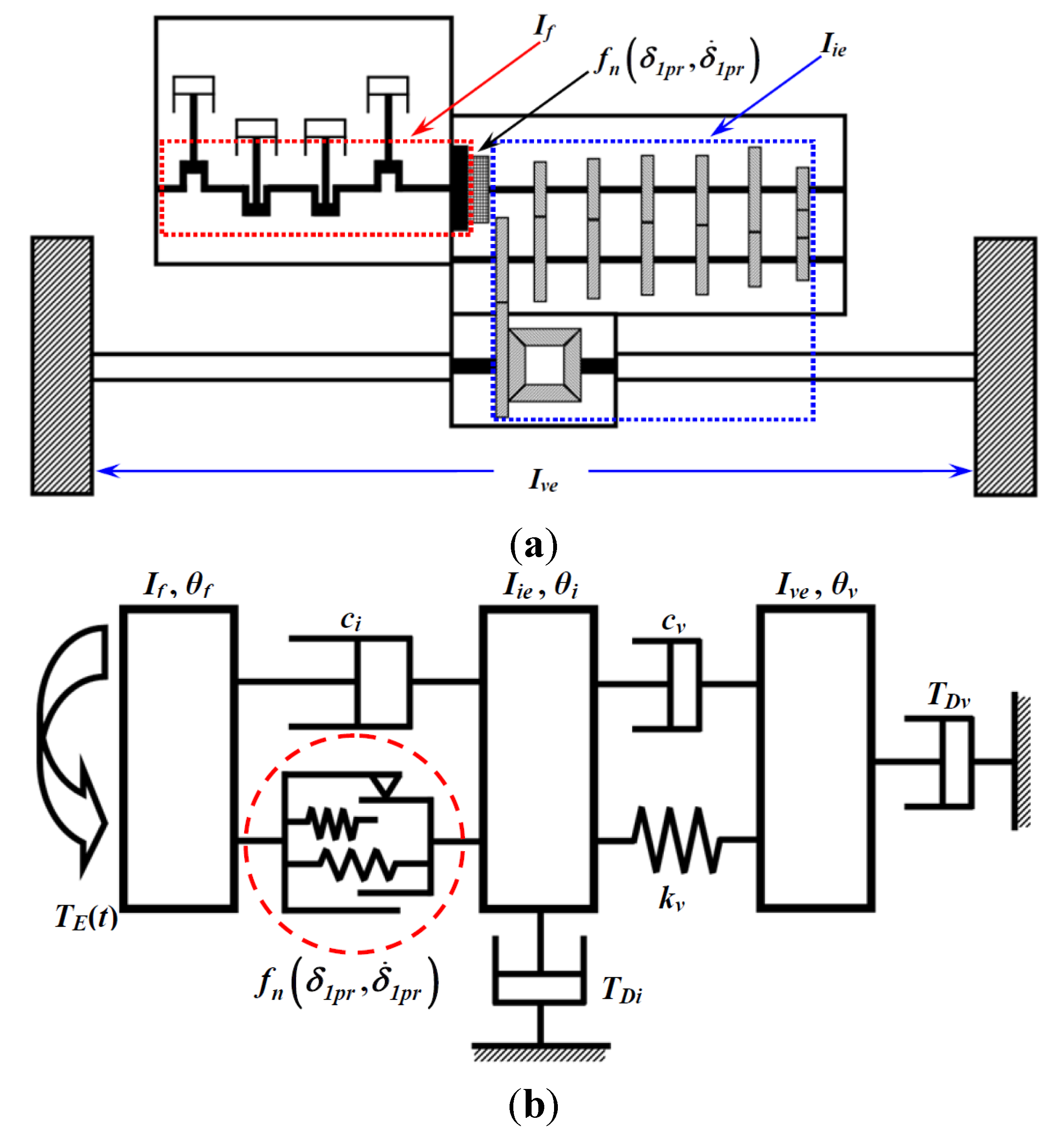
2. Problem Formulation

Figure 1 describes a practical system and its schematic diagram with 3DOF. The system is based on the front-engine and front-wheel type driveline system, which consists of an engine, clutch hub, engaged (or unloaded) gear, differential, drive shaft, and front wheel. These sub-systems can be modeled simply with a lumped nonlinear model, as shown in Figure 1b. The method of reducing the original system into a reduced-DOF system has been investigated in prior studies [1,2,3]. The symbols and their property values are as follows: If (=1.38 × 10⁻¹ kg·m2) is the inertia of the flywheel, which is lumped from the crank shaft and physical flywheel; Iie (=1.58 × 10⁻² kg·m2) is the inertia of the transmission, which is lumped from the input, output shafts, speed gears, and differential; Ive (=8.08 × 10⁻² kg·m2) is the inertia of the wheels and tires; kv (=3.95 × 10² N·m/rad) is the stiffness of the drive shaft; ci is the damping of the input shaft; cv is the damping of the wheel; TDi is the drag torque of the transmission; and TDv is the drag torque of the wheels. The employed drag torques vary with the different engine operating conditions, which will be explained later. In addition, ci and cv are assumed from the modal damping ratio of 1% [1,2,3,24].
Based on the schematic diagram shown in Figure 1b, the basic equations of motion are derived as follows:
M _ _ θ ¨ _ ( t ) + C _ _ θ ˙ _ ( t ) + K _ _ θ _ ( t ) + f n _ ( θ _ , θ ˙ _ ) = T E _ ( t )
M _ _ = d i a g [ I f , I i e , I v e ]
C _ _ = [ c i c i 0 c i c i + c v c v 0 c v c v ] , K _ _ = [ 0 0 0 0 k v k v 0 k v k v ]
f n _ ( θ _ , θ ˙ _ ) = [ f n ( δ 1 P r , δ ˙ 1 P r ) f n ( δ 1 P r , δ ˙ 1 P r ) + T D i T D v ] , T E _ ( t ) = [ T E ( t ) 0 0 ]
Here, the motion vector θ _ ( t ) = [ θ f θ i θ v ] T and θ f , θ i , and θ v are the displacements of the flywheel, transmission, and wheel, respectively. f n ( δ 1 P r , δ ˙ 1 P r ) is defined as a nonlinear function affected by multi-staged clutch dampers, which will be explained later. To investigate the nonlinear dynamic behaviors under various excitation conditions, the 3DOF torsional system in Figure 1 is assumed to be reduced under conditions with 3rd gear engaged and 5th gear unloaded [1,2,3]. The system responses will be examined under steady-state conditions using one-term harmonic torque profiles.
Figure 1. A practical driveline with a front-engine and front-wheel layout and a three degree-of-freedom (3DOF) nonlinear torsional system model with multi-staged clutch dampers: (a) physical driveline; and (b) schematic diagram with piecewise-type nonlinearities.
Energies 08 10861 g001

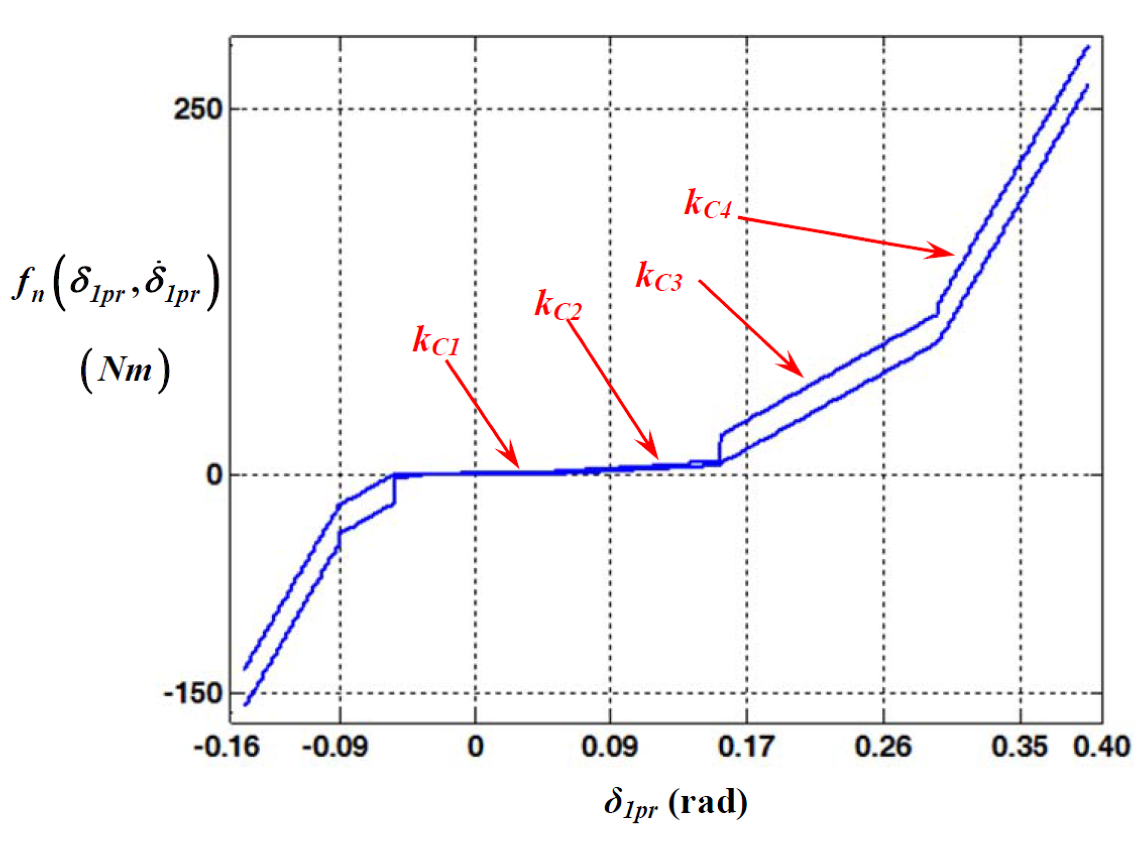
3. Nonlinear Analysis with Harmonic Balance Method and Piecewise-Type Nonlinearities

3.1. Harmonic Balance Method with Multi-Staged Clutch Dampers

In a prior study [24], the time responses for the ith sub-system θ i _ ( t ) were expanded based upon the Galerkin scheme as follows [24,25,26,27,28,29]:
θ i _ ( t ) = H _ _ θ ic _
θ i _ ( t ) = [ θ i ( t 0 ) θ i ( t 1 ) θ i ( t m 2 ) θ i ( t m 1 ) ]
θ ic _ = [ θ i m θ i a ( 1 ) θ i b ( 1 ) θ i a ( k ) θ i b ( k ) θ i a ( N max ) θ i b ( N max ) ] , H _ _ = [ 1 c o s ( k ρ ψ 0 ) s i n ( k ρ ψ 0 ) 1 c o s ( k ρ ψ 1 ) s i n ( k ρ ψ 1 ) 1 c o s ( k ρ ψ N 2 ) s i n ( k ρ ψ N 2 ) 1 c o s ( k ρ ψ N 1 ) s i n ( k ρ ψ N 1 ) ]
Here, ψ = ω t . From the relationships θ ˙ ( t ) = d θ d t = ω d θ d ψ = ω θ and θ ¨ ( t ) = ω 2 θ , the derivative of Equation (2d) is expressed as follows:
H _ _ = ω H _ _ P _ _ , H _ _ = ω 2 H _ _ P _ _
P _ _ = [ 0 [ 0 k / ρ k / ρ 0 ] ] , P _ _ = [ 0 [ ( k / ρ ) 2 0 0 ( k / ρ ) 2 ] ]
From Equations (1)–(3) with a multi-degree-of-freedom (MDOF) system model, the Galerkin scheme of the governing equations is expressed by the residual formulation as follows [14,24,25,26,27,28,29]:
ω 2 H t _ _ P t _ _ M t _ _ θ tc _ + ω H t _ _ P t _ _ C t _ _ θ tc _ + H t _ _ K t _ _ θ tc _ + f n _ ( θ _ , θ ˙ _ ) T E _ ( t ) = 0 _
θ tc _ = [ θ ic _ ] , H t _ _ = [ H _ _ ]
P t _ _ = [ P _ _ ] , P t _ _ = [ P _ _ ]
M t _ _ = [ I f I n _ _ 0 _ _ 0 _ _ 0 _ _ I i e I n _ _ 0 _ _ 0 _ _ 0 _ _ I v e I n _ _ ] , C t _ _ = [ c i I n _ _ c i I n _ _ 0 _ _ c i I n _ _ ( c i + c v ) I n _ _ c v I n _ _ 0 _ _ c v I n _ _ c v I n _ _ ]
K t _ _ = [ 0 _ _ 0 _ _ 0 _ _ 0 _ _ k v I n _ _ k v I n _ _ 0 _ _ k v I n _ _ k v I n _ _ ]
The subscript t is used for the overall matrix of the MDOF system constructed by the matrix at the ith sub-system, and I n _ _ is an identity matrix. The nonlinear function f n _ ( θ _ , θ ˙ _ ) and the input torque T E _ ( t ) at the ith sub-system can be expressed with the following equations in the same formulation as Equation (2):
f in _ ( θ i _ , θ ˙ i _ ) = H _ _ f ic _ , T iE _ ( t ) = H _ _ T ic _
f ic _ = [ f i m f i a ( 1 ) f i b ( 1 ) f i a ( k ) f i b ( k ) f i a ( ρ N max ) f i b ( ρ N max ) ] , T ic _ = [ T i m T i a ( 1 ) T i b ( 1 ) T i a ( k ) T i b ( k ) T i a ( ρ N max ) T i b ( ρ N max ) ]
From Equation (5), the overall f n _ ( θ _ , θ ˙ _ ) and T E _ ( t ) are as follows:
f n _ ( θ _ , θ ˙ _ ) = H t _ _ f tc _ , T E _ ( t ) = H t _ _ T tc _
f tc _ = [ f ic _ ] , T tc _ = [ T ic _ ]
Using Equations (5) and (6), Equation (4) can be expressed as follows:
ω 2 H t _ _ P t _ _ M t _ _ θ tc _ + ω H t _ _ P t _ _ C t _ _ θ tc _ + H t _ _ K t _ _ θ tc _ + H t _ _ f tc _ H t _ _ T tc _ = 0 _
Thus,
H t _ _ Ψ _ = 0 _ , Ψ _ = ω 2 P t _ _ M t _ _ θ tc _ + ω P t _ _ C t _ _ θ tc _ + K t _ _ θ tc _ + f tc _ F tc _ = 0 _
The Jacobian matrix J tc _ _ can be derived from Ψ _ as follows:
J tc _ _ = Ψ _ θ tc _ = ω 2 P t _ _ M t _ _ + ω P t _ _ C t _ _ + K t _ _ + f tc _ θ tc _
Since f tc _ θ tc _ for the whole system is difficult to estimate directly, f ic _ θ ic _ for the ith sub-system is obtained first by considering the derivative of both variables θ i _ ( t ) and θ ˙ i _ ( t ) [14,24]. Thus, f in _ ( θ i _ , θ ˙ i _ ) θ i _ ( t ) and f in _ ( θ i _ , θ ˙ i _ ) θ ˙ i _ ( t ) are defined with respect to the ith sub-system by diagonal matrices as follows:
f in _ ( θ i _ , θ ˙ i _ ) θ i _ ( t ) = d i a g [ f in _ ( θ i _ , θ ˙ i _ ) θ i _ ( t 0 ) f in _ ( θ i _ , θ ˙ i _ ) θ i _ ( t 1 ) f in _ ( θ i _ , θ ˙ i _ ) θ i _ ( t m - 2 ) f in _ ( θ i _ , θ ˙ i _ ) θ i _ ( t m - 1 ) ]
f in _ ( θ i _ , θ ˙ i _ ) θ ˙ i _ ( t ) = d i a g [ f in _ ( θ i _ , θ ˙ i _ ) θ ˙ i _ ( t 0 ) f in _ ( θ i _ , θ ˙ i _ ) θ ˙ i _ ( t 1 ) f in _ ( θ i _ , θ ˙ i _ ) θ ˙ i _ ( t m - 2 ) f in _ ( θ i _ , θ ˙ i _ ) θ ˙ i _ ( t m - 1 ) ]
Overall, both f n _ ( θ _ , θ ˙ _ ) θ _ ( t ) and f n _ ( θ _ , θ ˙ _ ) θ ˙ _ ( t ) are derived as follows:
f n _ ( θ _ , θ ˙ _ ) θ _ ( t ) = [ f 1n _ ( θ _ , θ ˙ _ ) θ 1 _ ( t ) f 1n _ ( θ _ , θ ˙ _ ) θ k _ ( t ) f kn _ ( θ _ , θ ˙ _ ) θ 1 _ ( t ) f kn _ ( θ _ , θ ˙ _ ) θ k _ ( t ) ] , f n _ ( θ _ , θ ˙ _ ) θ ˙ _ ( t ) = [ f 1n _ ( θ _ , θ ˙ _ ) θ ˙ 1 _ ( t ) f 1n _ ( θ _ , θ ˙ _ ) θ ˙ k _ ( t ) f kn _ ( θ _ , θ ˙ _ ) θ ˙ 1 _ ( t ) f kn _ ( θ _ , θ ˙ _ ) θ ˙ k _ ( t ) ]
From Equations (10) and (11), f tc _ θ tc _ can be expressed as follows:
f tc _ θ tc _ = H t _ _ + f n _ ( θ _ , θ ˙ _ ) θ _ ( t ) H t _ _ + ω H t _ _ + f n _ ( θ _ , θ ˙ _ ) θ ˙ _ ( t ) H t _ _ P t _ _
H t _ _ + = ( H t _ _ T H t _ _ ) 1 H t _ _ T
Here, H t _ _ + is a pseudoinverse matrix [14,24]. In addition, consider Ψ _ as a function of ω. The Jacobian matrix J ω _ is obtained by parameterizing the frequency ω on the basis of the arc-length continuation technique [14,24,25,26,27,28,29].
J ω _ = Ψ _ ω = ( 2 ω P t _ _ M t _ _ + P t _ _ C t _ _ + H t _ _ + f n _ ( θ _ , θ ˙ _ ) θ ˙ _ ( t ) H t _ _ P t _ _ ) θ tc _
Overall, the Jacobian matrix and the coefficient vector can be found as follows:
J _ _ = [ J tc _ _ J ω _ ] , θ a _ = [ θ tc _ ω ]
The Newton–Raphson method is employed by manipulating the following relationship:
θ a _ _ ( k + 1 ) = θ a _ _ ( k ) [ J _ _ + Ψ _ ( θ tc _ , ω ) ] ( k ) , J _ _ + = [ ( J _ _ T J _ _ ) 1 J _ _ T ]
Here, the nonlinear function affected by multi-staged clutch dampers is defined as follows [1,2,3,24]:
f n ( δ 1 P r , δ ˙ 1 P r ) = T S ( δ 1 P r ) + T H ( δ 1 P r , δ ˙ 1 P r ) + T P r ( δ 1 P r ) ,   δ 1 P r = δ 1 ϕ P r , δ 1 = θ f θ i
T S ( δ 1 P r ) = k C 1 δ 1 P r + 1 2 i = 2 N ( k C ( i ) k C ( i 1 ) ) ( D s p ( i 1 ) D s n ( i 1 ) )
D s p ( i ) = ( δ 1 P r ϕ p ( i ) ) [ t a n h { σ C ( δ 1 P r ϕ p ( i ) ) } + 1 ]
D s n ( i ) = ( δ 1 P r + ϕ n ( i ) ) [ t a n h { σ C ( δ 1 P r + ϕ n ( i ) ) } 1 ]
T H ( δ 1 P r , δ ˙ 1 P r ) = H ( N ) 2 t a n h ( σ H δ ˙ 1 P r ) + i = 2 N ( H ( i ) 4 H ( i 1 ) 4 ) [ D H p ( i 1 ) + D H n ( i 1 ) ]
D H p ( i ) = t a n h { σ C ( δ 1 P r ϕ p ( i ) ) } [ 1 + t a n h ( σ H δ ˙ 1 P r ) ]
D H n ( i ) = t a n h { σ C ( δ 1 P r + ϕ n ( i ) ) } [ 1 t a n h ( σ H δ ˙ 1 P r ) ]
T P r ( δ 1 P r ) = 1 2 T P r 1 [ t a n h ( σ C δ 1 P r ) + 1 ] + 1 2 T P r 2 [ t a n h ( σ C δ 1 P r ) + 1 ]
The nonlinear function f n ( δ 1 P r , δ ˙ 1 P r ) is composed of three clutch torques T S ( δ 1 P r ) , T H ( δ 1 P r , δ ˙ 1 P r ) , and T P r ( δ 1 P r ) , which are induced by the piecewise-linear stiffness with asymmetric transition angles, the hysteresis, and the preload, respectively. To overcome the convergence problems, smoothening factors σ C for the stiffness and σ H for the hysteresis are used with the values of 100 and 0.1, respectively [2]. In addition, TPr1 and TPr2 are the positive and negative torques induced by the preload, respectively, and ϕ P r is the angle where the preload is applied. In order to describe the smoothening change of δ 1 P r , hyperbolic tangent functions are used in Equations (17)–(19). KC(i) and H(i) indicate the clutch stiffness and the hysteresis at the ith clutch stage, Dsp(i) and Dsn(i) are the relative angular displacement on the positive and negative sides at the ith stage, DHp(i) and DHn(i) are the switching function at positive and negative angular displacements at the ith stage, and ϕ p ( i ) and ϕ n ( i ) are the ith transition angle on the positive and negative sides, respectively [1,2,3,24].
Table 1 describes the values employed for the multi-staged clutch dampers [1,2,3,24], and Figure 2 illustrates the dynamic characteristics of clutch torques along with the relative displacement between the flywheel and clutch transmission in terms of a nonlinear function f n ( δ 1 P r , δ ˙ 1 P r ) . The input torques are calculated by the Fourier components measured from the engine dynamometer test under the wide open throttle (WOT) condition. Thus, the input torque T E ( t ) with maximum harmonic terms Nmax is calculated using Tm and the alternating part of the engine torque Tpi as follows:
T E ( t ) = T m + i = 1 N max T p i c o s ( i ω p t + ϕ p i )
The torque profiles employed under various excitation conditions are listed in Table 2. The drag torques are estimated by assuming that the summation of drag torques TDi and TDv are equal to the mean torque value Tm. The calculation of drag torques along with the various operating conditions was presented in prior studies [1,2]. In the present study, the properties for the drag torques listed in Table 3 are used for each excitation condition.
Table 1. Properties of the practical multi-staged clutch dampers.
PropertyStageValue
Torsional stiffness, kC (linearized in a piecewise manner) (N·m/rad)110.1
261.8
3595.8
41838.0
Hysteresis, Hi (N·m)10.98
21.96
319.6
426.5
Transition angle at positive side (δi > 0), ϕ p i (rad)10.05
20.16
30.30
40.39
Transition angle at negative side (δi < 0), ϕ n i (rad)1−0.04
2−0.05
3−0.09
4−0.15
Table 2. List of the input torque profiles under various excitation conditions.
Torque ComponentCase ICase IICase III
Magnitude (N·m)TM160.8192.3195.9
Tp1357.6589.61378.6
Phase (rad) ϕ p 1 −1.86−1.71−1.64
Table 3. List of the drag torque profiles under various excitation conditions.
Torque ComponentCase ICase IICase III
TDi (N·m)14.946.550.1
TDv (N·m)145.8145.8145.8
Figure 2. Clutch torque profile of multi-staged clutch dampers with the nonlinear function f n ( δ 1 P r , δ ˙ 1 P r ) .
Energies 08 10861 g002

3.2. Examination of System Responses of Severe Excitation Condition

Figure 3, Figure 4 and Figure 5 show the simulation results obtained using the HBM compared with those of the linear analysis. In order to investigate the nonlinear dynamic characteristics in the practical system of Figure 1, the input conditions described in Table 2 are employed with Case III.
As shown in Figure 3, the root-mean-square (RMS) values of the relative displacement in the frequency domain deviate from the resonance regime of the linear analysis. δ 1 ( t ) is the relative displacement between the flywheel and transmission, and δ 2 ( t ) is that between the transmission and the wheel. In addition, the RMS values δ 1 ( r m s ) and δ 2 ( r m s ) are calculated using Equation (21a) and Equation (21b), respectively.
δ 1 ( r m s ) = 1 m { δ 1 2 ( t 0 ) + δ 1 2 ( t 1 ) + + δ 1 2 ( t m 1 ) }
δ 2 ( r m s ) = 1 m { δ 2 2 ( t 0 ) + δ 2 2 ( t 1 ) + + δ 2 2 ( t m 1 ) }
The unstable regimes are found around the normalized frequency values of 0.7, 0.9, and 1.3. The stability analysis is determined by Hill’s method [14,24,30]. When the dynamic responses are examined at these unstable zones, jumping phenomena are clearly observed, especially in Figure 3b. Thus, the practical driveline system shows two different areas of jumping phenomena while the system is excited under frequency up- or down-sweeping conditions, which will be explained in more detail later.
Figure 3. Comparison of root-mean-square (RMS) values of relative displacement between nonlinear and linear analysis: (a) RMS values of δ 1 ( t ) and (b) RMS values of δ 2 ( t ) . Key: ━━, linear analysis; Energies 08 10861 i001, harmonic balance method (HBM) (stable solution); Energies 08 10861 i002, HBM (unstable solution).
Energies 08 10861 g003
The nonlinear dynamic characteristics can also be examined by comparing the linear analysis in the Poincaré maps, as shown in Figure 4 and Figure 5. The Poincaré map is determined based on the HBM by assuming that the levels of δ 1 ( t i , ω ¯ ) and δ 2 ( t i , ω ¯ ) are perfectly the same as those of δ 1 ( t i + n T , ω ¯ ) and δ 2 ( t i + n T , ω ¯ ) , respectively. The subscript i indicates the series of discretized time data from 0 to m-1, as described in Equation (2b). n and T are the number of cycles and the period, respectively, under varying excitation frequency ω.
Figure 4. Comparison of Poincaré maps between nonlinear and linear models: (a) Poincaré map of δ 1 ( t i + n T , ω ¯ ) vs. δ ˙ 1 ( t i + n T , ω ¯ ) in the frequency domain; and (b) Poincaré map of δ 2 ( t i + n T , ω ¯ ) vs. δ ˙ 2 ( t i + n T , ω ¯ ) in the frequency domain. Key: ━━, linear analysis; , HBM (stable solution); Energies 08 10861 i002, HBM (unstable solution).
Energies 08 10861 g004
Figure 4 and Figure 5 are determined with the value i = 1 under the frequency sweeping conditions. When the nonlinear and linear analyses are compared as shown in Figure 4, the nonlinear responses show abrupt changes of the relative motions including unstable zones. However, it is difficult to observe any jumping phenomena or unstable regimes in the linear analysis. The scale of the system responses in the nonlinear analysis is smaller than that in the linear analysis. This is also clearly observed in Figure 5 with only the relationships of δ 1 ( t i + n T , ω ¯ ) or δ 2 ( t i + n T , ω ¯ ) vs. δ ˙ 1 ( t i + n T , ω ¯ ) or δ ˙ 2 ( t i + n T , ω ¯ ) . The comparison shown in Figure 5 reveals that the range of the nonlinear dynamic behaviors is reduced in all the frequency ranges. The directions of the stable and unstable conditions are also predicted for δ 1 ( t ) and δ 2 ( t ) , which makes it possible to anticipate the range of the practical system responses.
Figure 5. Comparison of Poincaré maps between nonlinear and linear models: (a) Poincaré map of δ 1 ( t i + n T , ω ¯ ) vs. δ ˙ 1 ( t i + n T , ω ¯ ) along with the excitation frequency; and (b) Poincaré map of δ 2 ( t i + n T , ω ¯ ) vs. δ ˙ 2 ( t i + n T , ω ¯ ) along with the excitation frequency. Key: ━━, linear analysis; , HBM (stable solution); Energies 08 10861 i002, HBM (unstable solution).
Energies 08 10861 g005
Regarding the nonlinear dynamic responses observed in the Poincaré map shown in Figure 5 and Figure 6, the jumping phenomena at the unstable regimes can also clearly be found in the frequency domain, as shown in Figure 6 and Figure 7. When Figure 6 is examined with respect to the relative displacement δ 1 ( t ) , the back bone curve bends into the left side first, and then it turns over to the right side. Thus, it has two jumping areas that are dependent on the frequency sweeping directions. The jumping locations marked by the dotted lines in Figure 6a are shown in more detail in Figure 6b, where the arrows marked by the solid lines indicate the frequency up-sweeping track. The dotted arrows illustrate the dynamic behaviors under down-sweeping frequency. Figure 7 shows the same dynamic behaviors for the relative displacement δ 2 ( t ) as those of δ 1 ( t ) . The comparison of both the HBM and numerical simulation (NS) results are well correlated, as shown in Figure 6 and Figure 7.
Figure 6. Comparison of HBM (Nmax = 12 and ρ = 1) with NS in the frequency domain: (a) comparison of max, mean, and min values of δ 1 ( t ) ; (b) illustration of jumping phenomena under the frequency up- and down-sweeping conditions. Key: ━━, HBM; Energies 08 10861 i001, NS by frequency up-sweeping; Energies 08 10861 i002, NS by frequency down-sweeping; , flow of numerical solution under frequency up-sweeping; ·······› , flow of numerical solution under frequency down-sweeping.
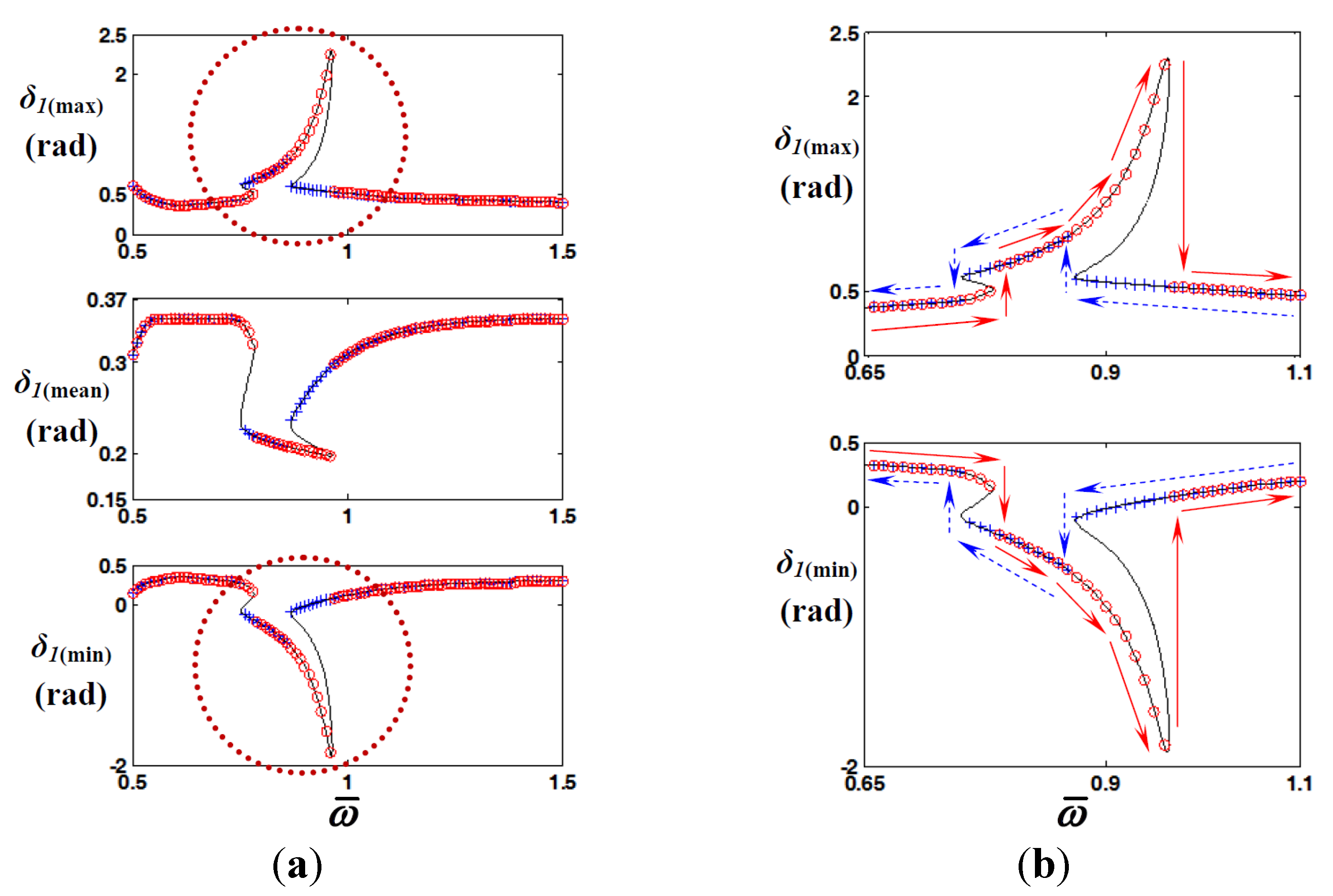
Energies 08 10861 g006
Figure 7. Comparison of HBM (Nmax = 12 and ρ = 1) with NS in the frequency domain: (a) comparison of max, mean, and min values of δ 2 ( t ) ; and (b) illustration of jumping phenomena under the frequency up- and down-sweeping conditions. Key: ━━, HBM; Energies 08 10861 i001, NS by frequency up-sweeping; Energies 08 10861 i002, NS by frequency down-sweeping.
Energies 08 10861 g007

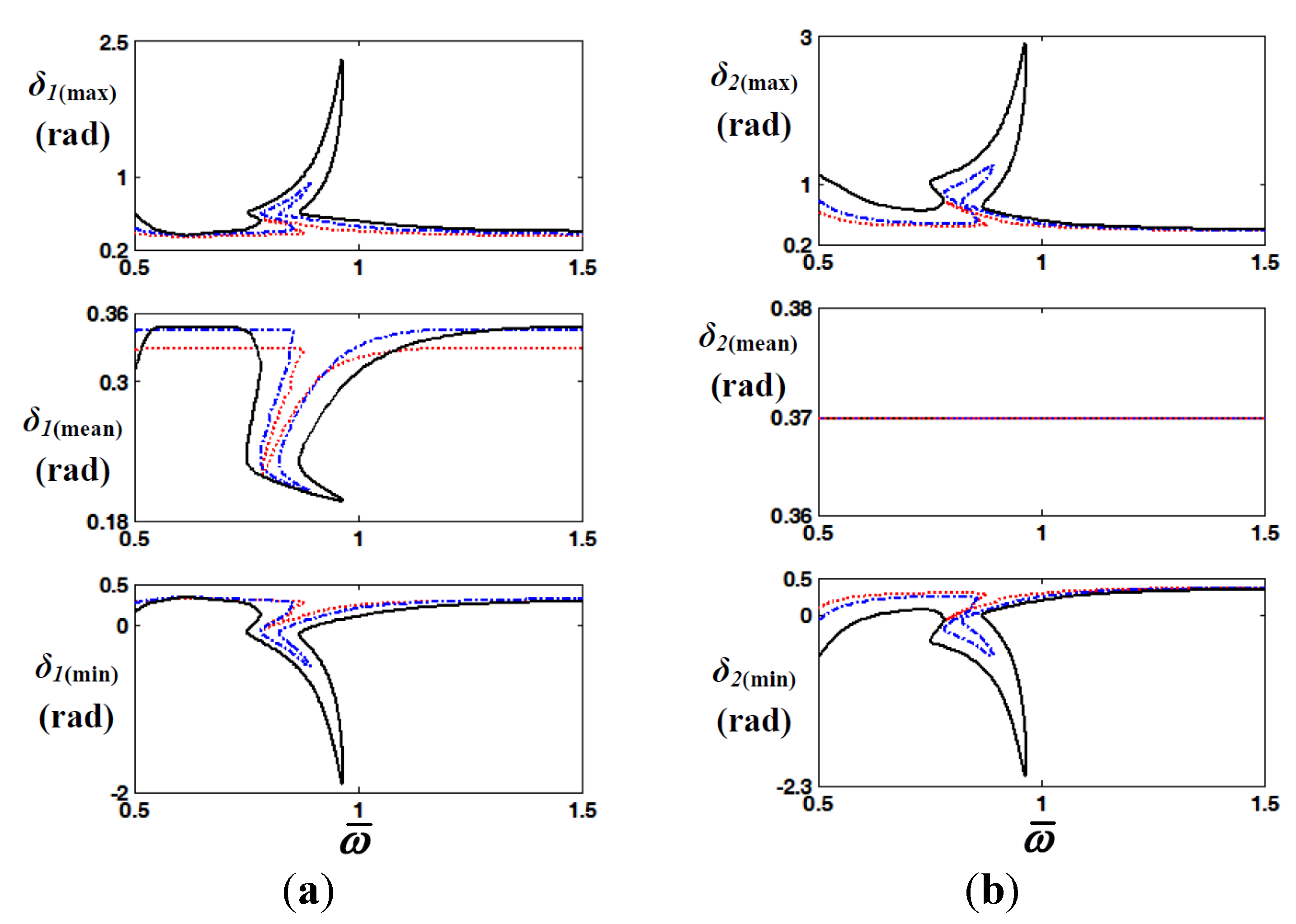
4. Nonlinear Dynamic Responses along with Various Excitation Conditions

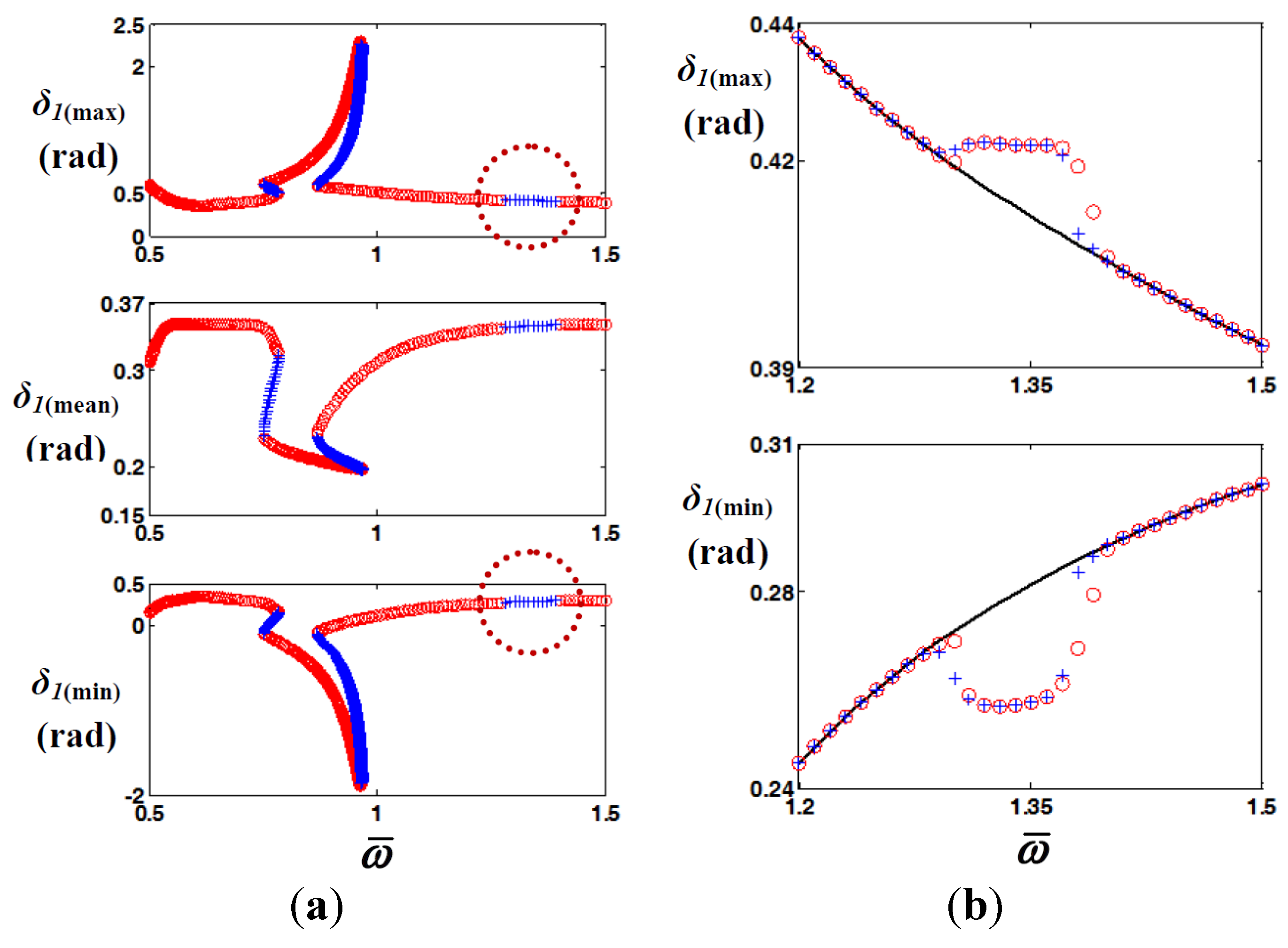
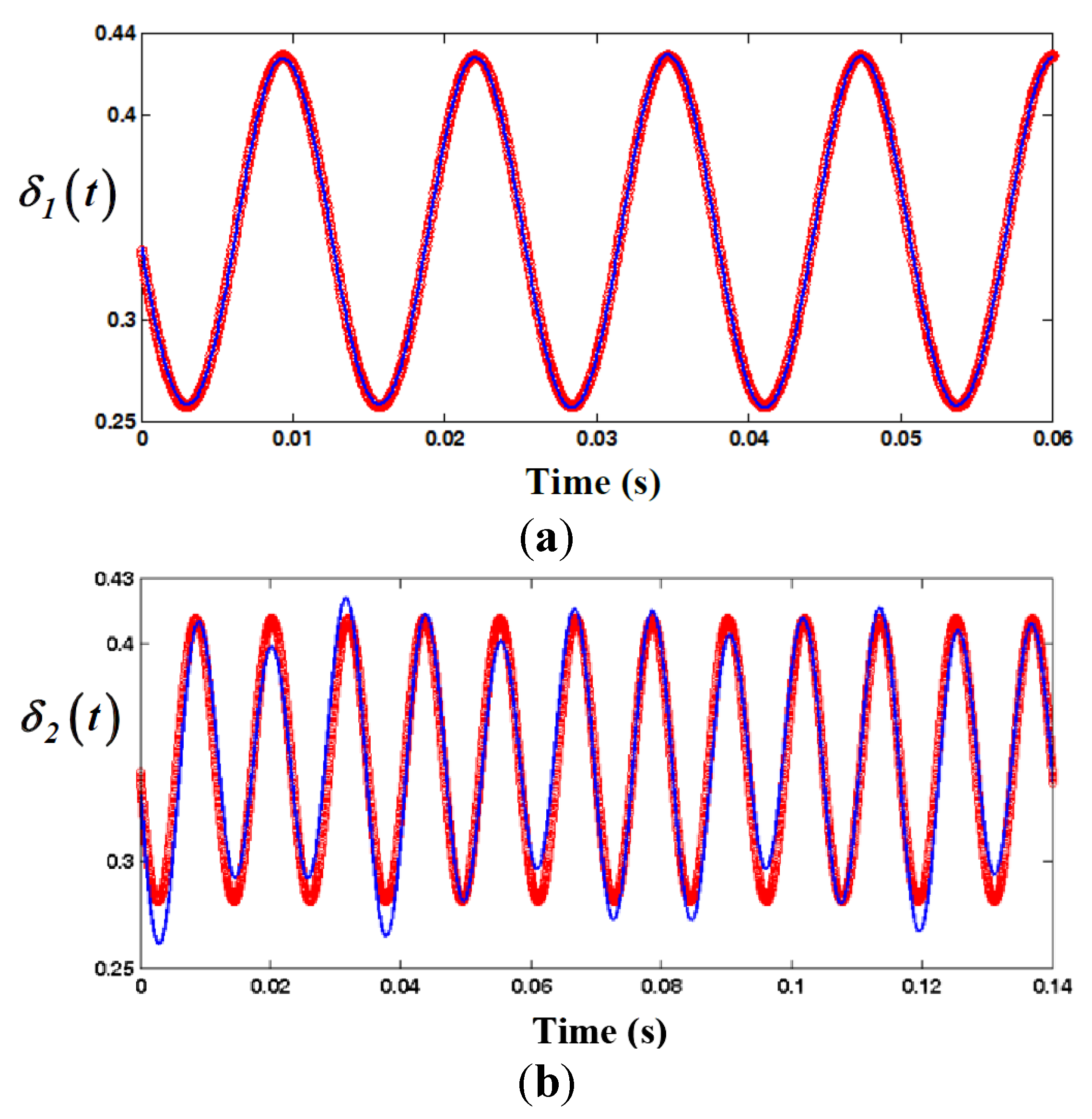
4.1. Nonlinear Dynamic Characteristics with Various Excitation Conditions

In a prior study, in general, nonlinear dynamic responses show diverse characteristics with various excitation conditions [16]. For example, it might have left or right simply bent shapes of the frequency responses with one jumping range, or it might include more than two jumping phenomena, as investigated in Section 3. Figure 8, Figure 9 and Figure 10 compare the nonlinear dynamic behaviors with various input conditions. The torque profiles employed are listed in Table 2 and Table 3. Table 2 describes three engine torque profiles under different engine operating conditions. For example, Case I is the measured engine torque data under the WOT condition at 1500 RPM. Since the Inline 4 (I4) cylinder type engine is employed, the firing frequency is 50 Hz. The engine torque data for Cases II and III are also measured at 3000 and 6000 RPM under the WOT condition. In order to measure the practical engine torque profile, an engine dynamometer test can be conducted [1,2,3]. In addition, various drag torques are employed instead of constant ones, since the drag torque for the input shaft TDi changes with the operating speed of the input shaft, as listed in Table 3. The drag torque was calculated as suggested by prior studies [1,2,3].
Figure 8 compares the maximum, mean, and minimum values of time histories along with frequency values under the various excitation conditions. Thus, as the engine excitation conditions become severe, the shape of the nonlinear frequency response becomes complicated. For example, the nonlinear responses for both δ 1 ( t ) and δ 2 ( t ) with Case I are bent to the left side, as indicated by the dotted line in Figure 8. This means that the backbone curve simply bends over to the left side, while the maxima of the resonances are increased. However, the backbone curves with Cases II and III follow similar paths to Case I first, and then they change direction to the right side, which increases the regimes of jumping phenomena twice, as described in Section 3. Thus, this simulation results reveal that the nonlinear dynamic responses have similar characteristics to the results in a prior study [16]. This leads to understanding of the dynamic characteristics of sub-systems affected by the excitation input levels and the local forces.
The dynamic behaviors of the sub-system in terms of the relative motions can be examined by using Poincaré maps as well, which are shown in Figure 9 and Figure 10. These Poincaré maps are simulated by the same method and event described in Section 3. The track of the simulation result for Case I illustrated by a dotted line in Figure 9 shows a simply bent shape. However, those for Cases II and III follow more complicated tracks, as clearly shown in Figure 9. The scale of dynamic responses with Cases II and III are also broader than the one for Case I as the excitation levels are increased. This is shown clearly in Figure 10 as well. Thus, using the Poincaré map gives useful information with respect to the dynamic characteristics of sub-systems in terms of relative motions.
Figure 8. Comparison of the HBM (Nmax = 12 and ρ = 1) results along with different excitation conditions in the frequency domain: (a) comparison of max, mean, and min values of δ 1 ( t ) ; and (b) comparison of max, mean, and min values of δ 2 ( t ) . Key: ········· , Case I; ─ · ─ , Case II; ━━, Case III.
Energies 08 10861 g008
Figure 9. Comparison of Poincaré maps along with different excitation conditions: (a) Poincaré map of δ 1 ( t i + n T , ω ¯ ) vs. δ ˙ 1 ( t i + n T , ω ¯ ) in the frequency domain; and (b) Poincaré map of δ 2 ( t i + n T , ω ¯ ) vs. δ ˙ 2 ( t i + n T , ω ¯ ) in the frequency domain. Key: ∙∙∙∙∙∙∙∙∙, Case I; ------- , Case II; ━━ , Case III.
Energies 08 10861 g009
Figure 10. Comparison of Poincaré maps under different excitation conditions: (a) Poincaré map of δ 1 ( t i + n T , ω ¯ ) vs. δ ˙ 1 ( t i + n T , ω ¯ ) in the frequency domain; amd (b) Poincaré map of δ 2 ( t i + n T , ω ¯ ) vs. δ ˙ 2 ( t i + n T , ω ¯ ) in the frequency domain. Key: ∙∙∙∙∙∙∙∙∙, Case I; ------- , Case II; ━━ , Case III.
Energies 08 10861 g010
First, the tracks of dynamic behaviors can be found clearly including the range of dynamic motions simultaneously. Second, the ranges of dynamic motions can be analyzed effectively as shown in Figure 10. In addition, the practical response areas corresponding to the stable regimes can be predicted as shown in Figure 5, since these results are based on the HBM including Hill’s method [14,24,30].

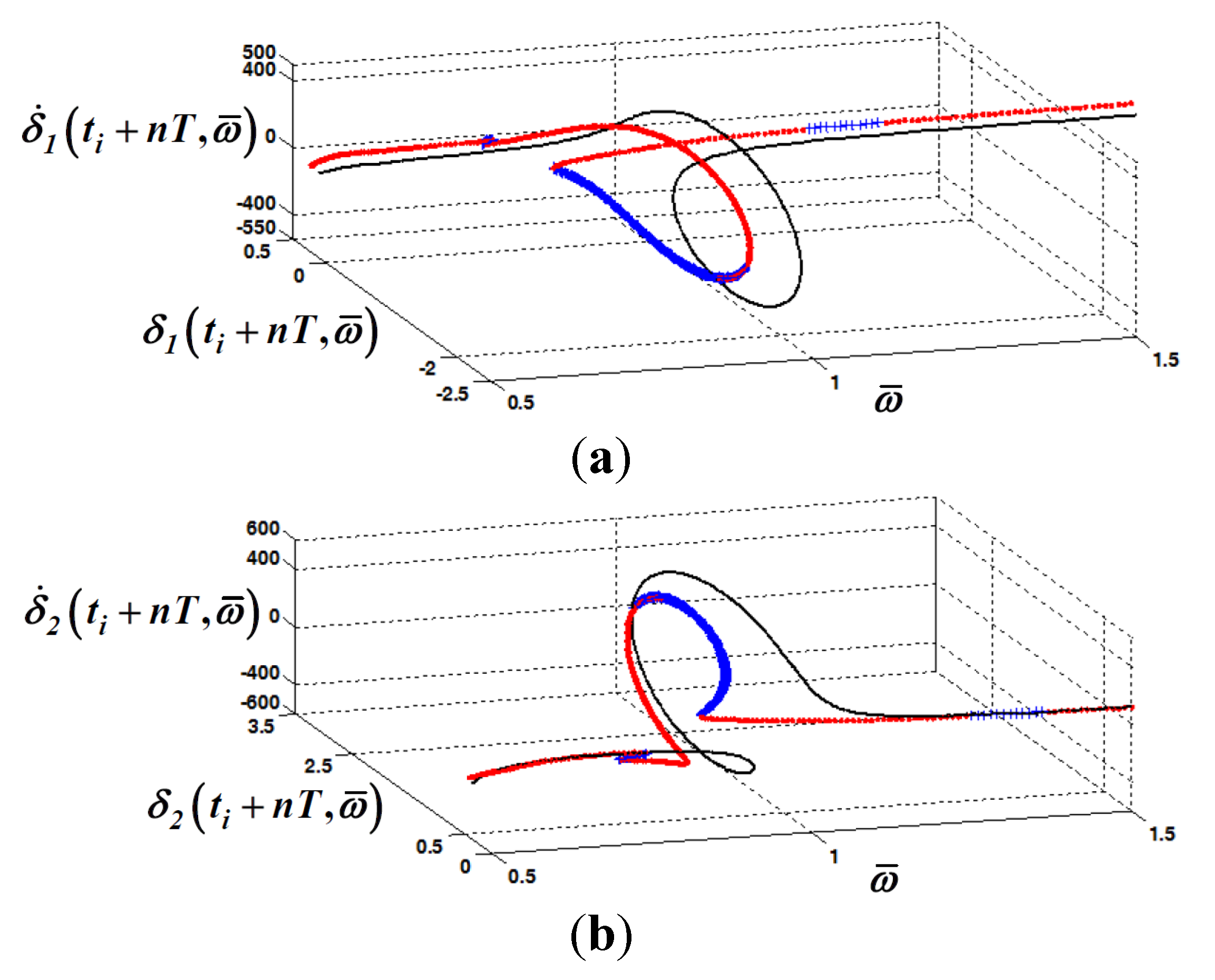
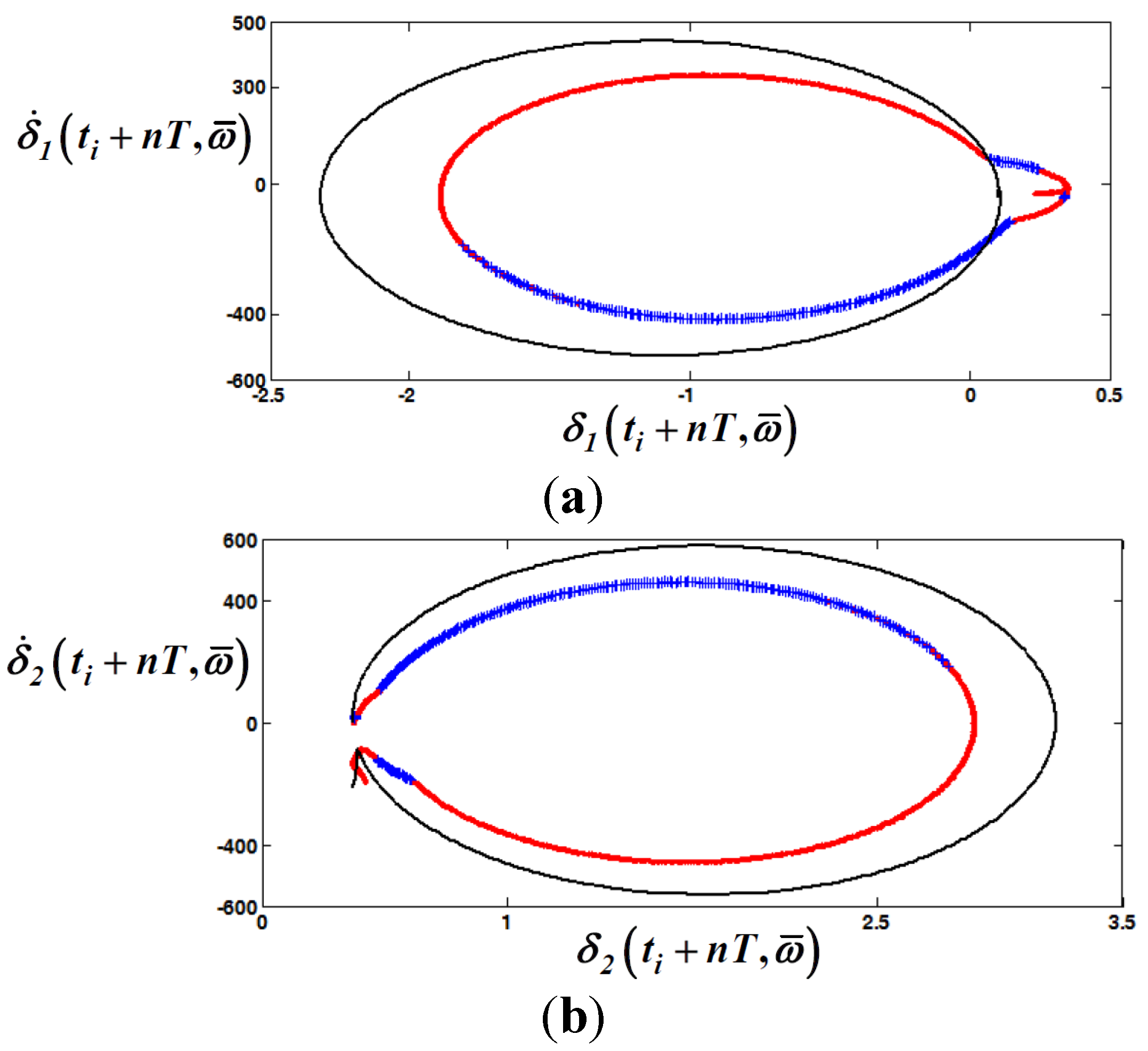
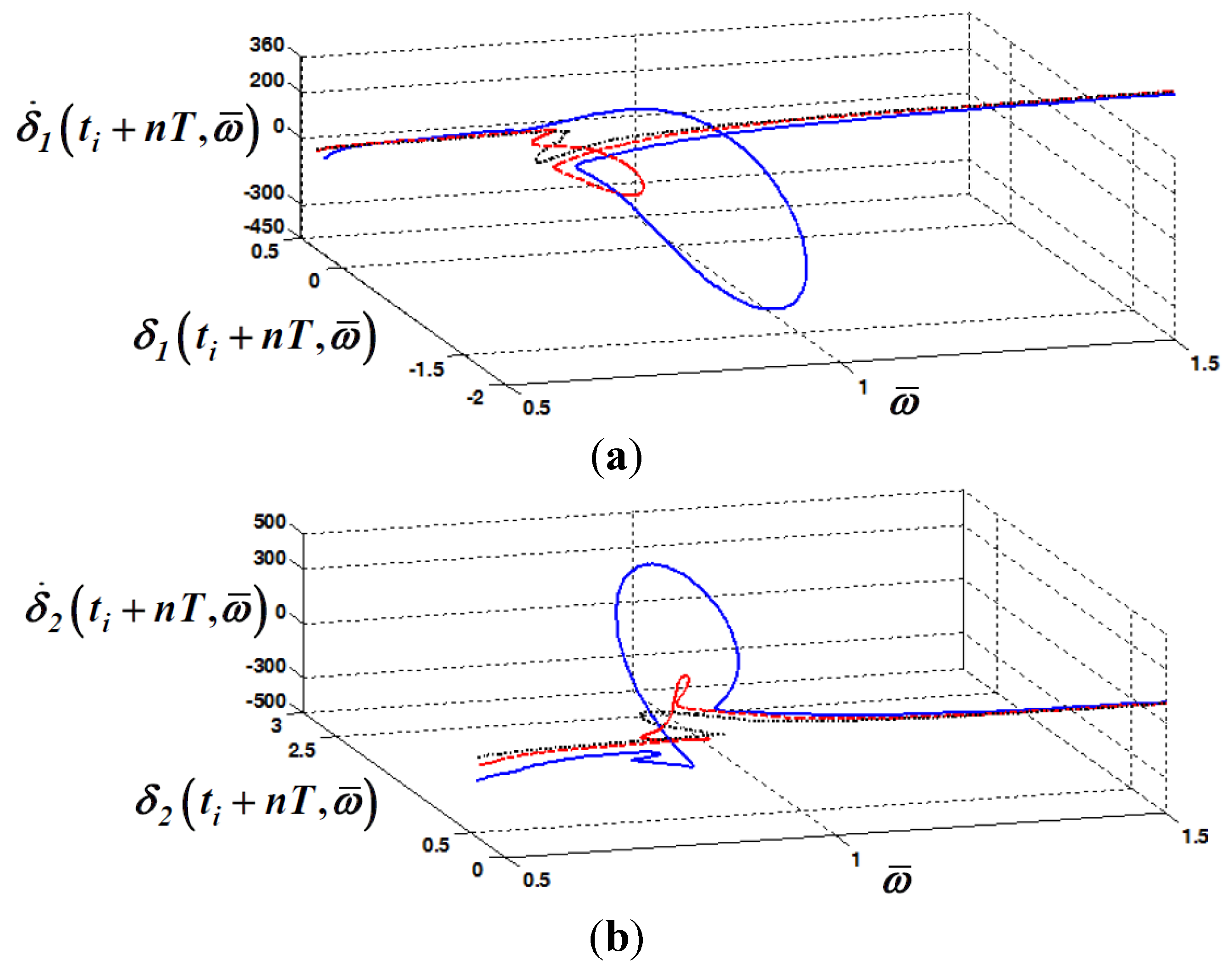
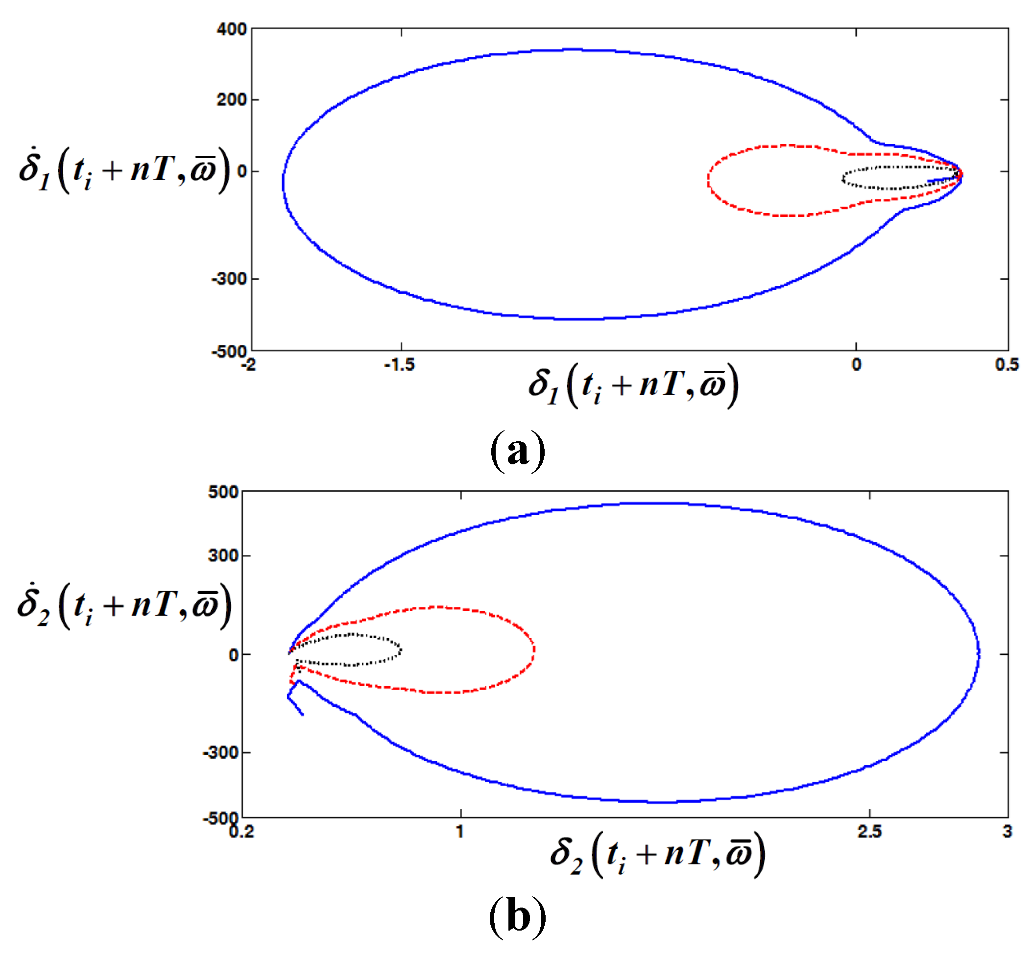
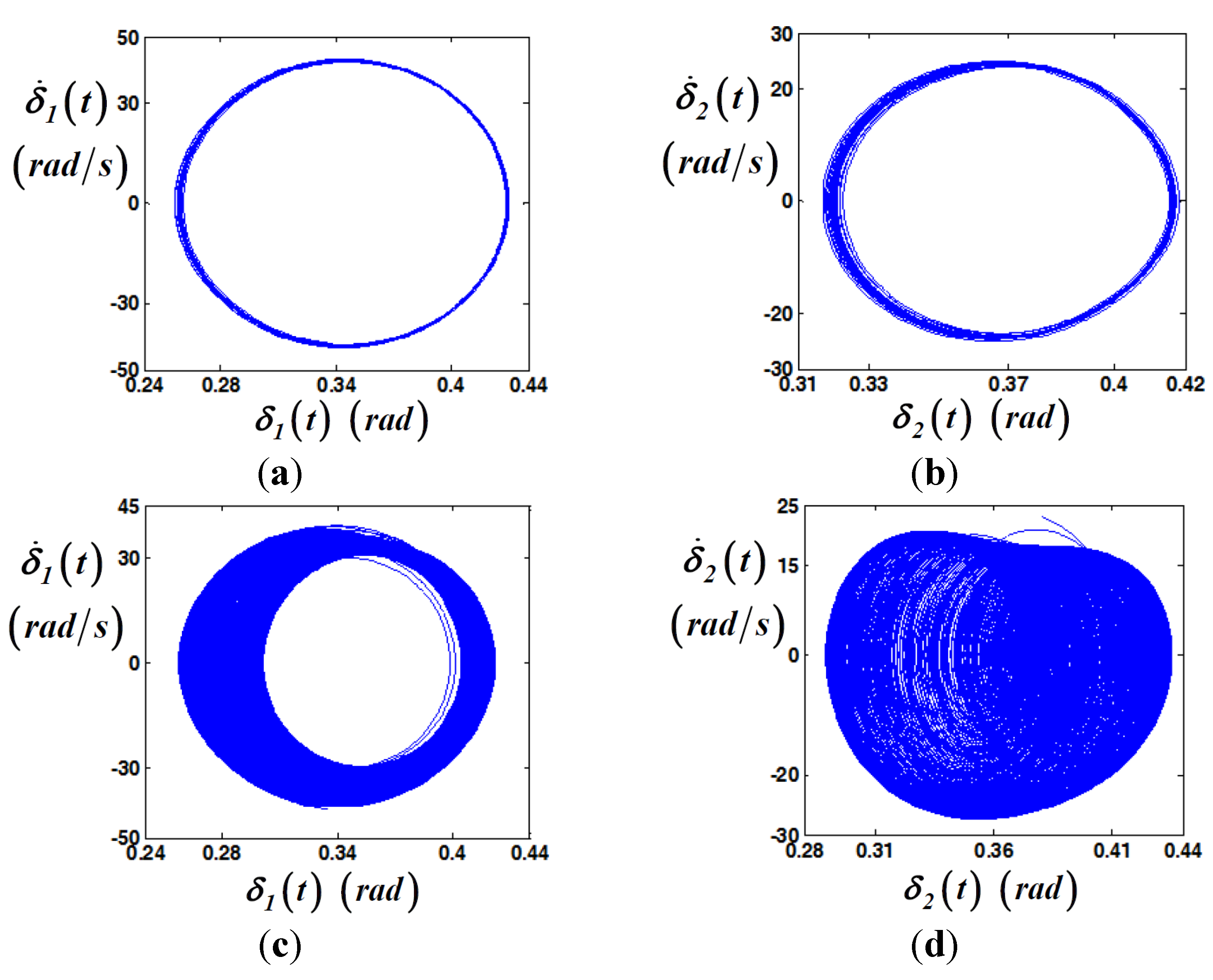
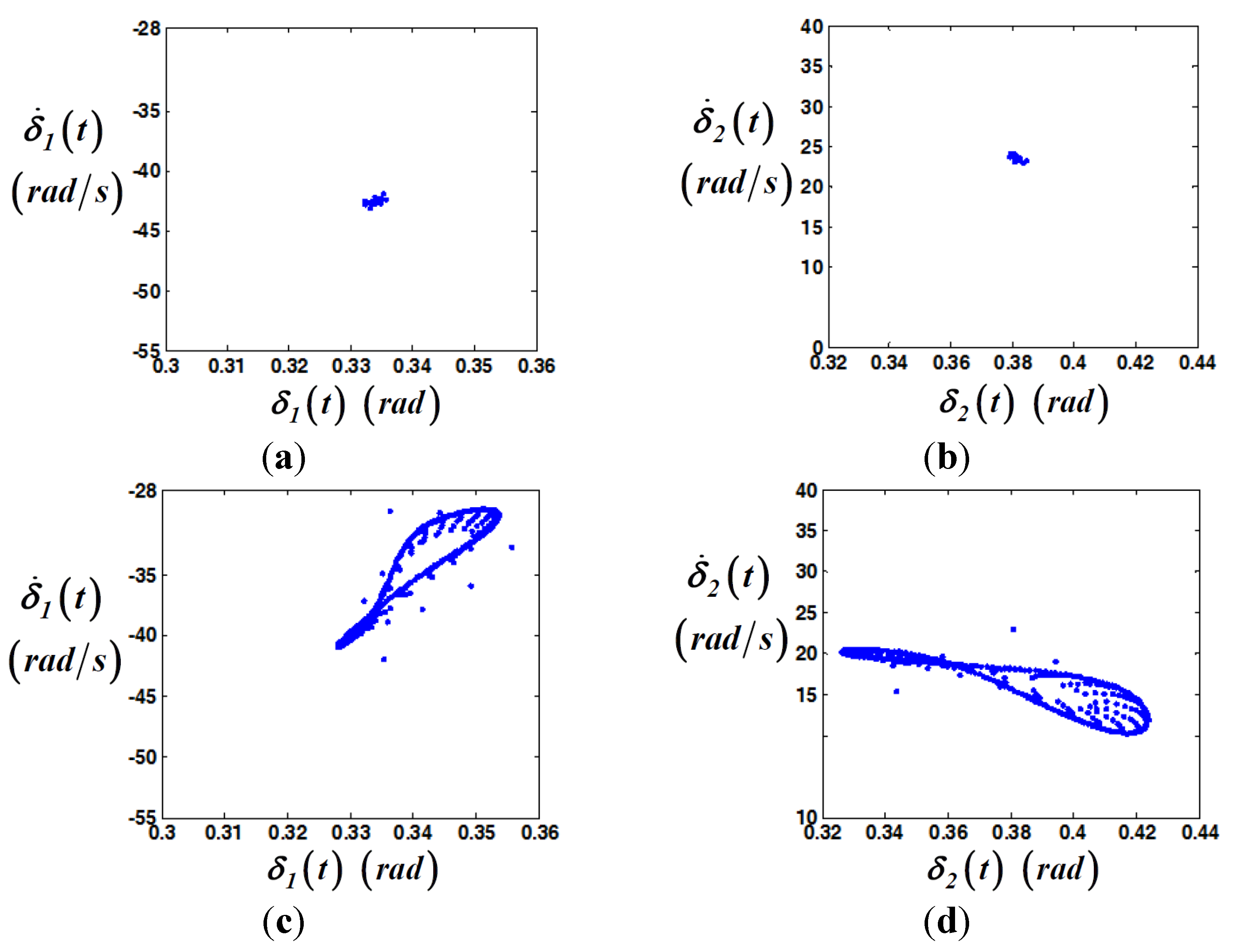
4.2. Investigation of Quasi-Periodic Responses Using Poincaré Map

Figure 11 and Figure 12 compare the HBM and NS by focusing on the unstable regime, which includes the quasi-periodic responses. When the nonlinear responses of the HBM are compared with those by NS, it is hard to expect quasi-periodic responses using only the HBM, since the matrix of harmonic terms is constructed on an integer basis [24]. However, the stability analysis using the HBM still gives information indicating that it is unstable, with the dynamic behaviors composed of random or quasi-periodic components. Thus, these unstable components or time responses need to be examined simultaneously based on the NS, as shown in Figure 11 and Figure 12. Figure 11 shows the comparison of the HBM with NS. In the unstable regime, both HBM and NS show differences, with the HBM not being able to anticipate all of the quasi-periodic components. The effect from the quasi-periodic components is clearly shown in the time histories in Figure 12. Figure 12a shows good correlations between HBM and NS. However, the time histories in the unstable regime in Figure 12b show differences between HBM and NS. In addition, quasi-periodic responses are found in the NS result.
Figure 11. Comparison of results from HBM (Nmax = 12 and ρ = 1) and NS at the unstable regime: (a) max, mean, and min values of δ 1 ( t ) from HBM results; and (b) comparison of HBM and NS under the unstable regime. Key: ━━, HBM; Energies 08 10861 i001, HBM with stable regime (or NS by frequency up-sweeping); Energies 08 10861 i002, HBM with unstable regime (or NS by frequency down-sweeping).
Energies 08 10861 g011
Figure 12. Time histories by HBM (Nmax = 12 and ρ = 1) and NS at different excitation conditions: (a) time histories at ω ¯ = 1.25; and (b) time histories at ω ¯ = 1.35. Key: Energies 08 10861 i001, HBM; ━━ , NS.
Energies 08 10861 g012
Figure 13 and Figure 14 suggest another way to investigate the nonlinear dynamic behaviors for the unstable responses. These results are based on the NS. Figure 13 compares the phase planes for the stable and unstable regimes with the relationship of δ 1 ( t ) vs. δ ˙ 1 ( t ) (or δ 2 ( t ) and δ ˙ 2 ( t ) ). As shown in Figure 13a,b, the tracks of the phase plane are within a limited boundary. Thus, the system responses are predictable as long as the excitation frequency levels are fixed. However, the tracks of the system responses in the phase plane become broader and hard to anticipate, as shown in Figure 13c,d. In general, the quasi-periodic responses contain many harmonic components and need more than two times the period in order to determine all the effective harmonic components. In addition, there are different components for each period, which makes the tracks of the phase plane for the unstable case denser and more unpredictable than those for the stable case.
Figure 13. Comparison of phase planes at different excitation conditions: (a) phase plane with δ 1 ( t ) vs. δ ˙ 1 ( t ) at ω ¯ = 1.25; (b) phase plane with δ 2 ( t ) vs. δ ˙ 2 ( t ) at ω ¯ = 1.25; (c) phase plane with δ 1 ( t ) vs. δ ˙ 1 ( t ) at ω ¯ = 1.35 ; and (d) phase plane with δ 2 ( t ) vs. δ ˙ 2 ( t ) at ω ¯ = 1.35.
Energies 08 10861 g013
When the quasi-periodic is examined using a Poincaré map, the dynamic characteristics are observed clearly, as shown in Figure 14. In order to find the Poincaré map for the fixed excitation frequency level, the NS results are mapped by assuming that δ 1 ( t i ) δ 1 ( t i + n T ) or δ 2 ( t i ) δ 2 ( t i + n T ) . Here, the subscript value i = 1 is employed with a fixed normalized frequency level of 1.35. In Figure 14a,b, the Poincaré map from the NS result is limited to a very small range of area.
Figure 14. Comparison of Poincaré maps at different excitation conditions: (a) Poincaré map with δ 1 ( t ) vs. δ ˙ 1 ( t ) at ω ¯ = 1.25; (b) Poincaré map with δ 2 ( t ) vs. δ ˙ 2 ( t ) at ω ¯ = 1.25; (c) Poincaré map with δ 1 ( t ) vs. δ ˙ 1 ( t ) at ω ¯ = 1.35; and (d) Poincaré map with δ 2 ( t ) vs. δ ˙ 2 ( t ) at ω ¯ = 1.35.
Energies 08 10861 g014
Ideally, it is limited to one point. Figure 14c,d shows different shapes of the Poincaré map, which has a wider range of tracks, even though it is drawn from each periodic time history. Thus, the differences of system responses with periodic and quasi-periodic components are revealed in very different ways in the Poincaré maps. Also, the quasi-periodic responses show random behaviors, as shown in Figure 14c,d. These results lead to similar trends of quasi-periodic responses to those in the other types of systems [5,18].

5. Conclusions

The effect of various excitation conditions on practical systems was studied using piecewise-type nonlinearities. In order to investigate the nonlinear dynamic behaviors, multi-staged clutch dampers were modeled, and the relative motions were examined with different input conditions. The contributions of this study are summarized as follows. First, the trends of nonlinear dynamic responses with various engine excitation conditions have been investigated. Two different regimes of jumping phenomena with up- and down-sweeping conditions of the frequency were investigated under an extremely large scale of excitation values. Second, Poincaré map models have been suggested for the system. The differences between the linear and nonlinear models (or nonlinear responses along with different excitation conditions) were examined, including the dynamic characteristics under stable and unstable frequency ranges. Third, quasi-periodic responses of the practical system in the unstable regime have been examined in both the frequency and time domains using HBM and NS. A comparison of dynamic behaviors in the stable and unstable frequency regimes using phase planes and Poincaré maps led to clear understanding of the nonlinear dynamic responses.
This study has investigated the nonlinear dynamic responses of sub-systems from the effect of piecewise-type nonlinearities. However, the practical system shows many nonlinear dynamics affected by clearance-type nonlinearities such as gear backlash. Further study will be done as an extension of this work. For the validation of the study, this method needs to be correlated with realistic experiments (physical driveline and a torsional exciter) based on time-domain data including the development of adapted simulation method for the wind turbine, which is a subject for future study. Overall, based on the scope of this study, it will lead to understanding the geared system and giving the basic concepts to develop the simulation method of highly nonlinear system such as wind turbine.

Acknowledgments

This work was supported by the research grant of the Kongju National University in 2015 (2015-0637-01) and the 2014 Yeungnam University Research Grant (214A054011).

Author Contributions

Jong-yun Yoon and Byeongil Kim initiated and developed the ideas related to this research work. Jong-yun Yoon and Byeongil Kim developed novel methods, derived relevant formulations, and carried out performance analyses and numerical analyses. Jong-yun Yoon wrote the paper draft under Byeongil Kim’s guidance and Byeongil Kim finalized the paper.

Conflicts of Interest

The authors declare no conflict of interest.

References

  1. Yoon, J.Y.; Singh, R. Effect of multi-staged clutch damper characteristics on transmission gear rattle under two engine conditions. J. Automob. Eng. 2013, 227, 1273–1294. [Google Scholar] [CrossRef]
  2. Yoon, J.Y.; Lee, I.J. Nonlinear analysis of vibro-impacts for unloaded gear pairs with various excitation and system parameters. J. Vib. Acoust. 2014, 136. [Google Scholar] [CrossRef]
  3. Yoon, J.Y. Effect of multi-staged clutch damper characteristics on vibro-impacts within a geared system. Master’s Thesis, Ohio State University, Columbus, OH, USA, 2003. [Google Scholar]
  4. Peng, Z.K.; Lang, Z.Q.; Billings, S.A.; Tomlinson, G.R. Comparison between harmonic balance and nonlinear output frequency response function in nonlinear system analysis. J. Sound Vib. 2008, 311, 56–73. [Google Scholar] [CrossRef]
  5. Al-shyyab, A.; Kahraman, A. Non-linear dynamic analysis of a multi-mesh gear train using multi-term harmonic balance method: Sub-harmonic motions. J. Sound Vib. 2005, 279, 417–451. [Google Scholar] [CrossRef]
  6. Chen, Y.M.; Liu, J.K.; Meng, G. Incremental harmonic balance method for nonlinear flutter of an airfoil with uncertain-but-bounded parameters. Appl. Math. Model. 2012, 36, 657–667. [Google Scholar] [CrossRef]
  7. Genesio, R.; Tesi, A. Harmonic balance methods for the analysis of chaotic dynamics in nonlinear systems. Automatica 1992, 28, 531–548. [Google Scholar] [CrossRef]
  8. Masiani, R.; Capecchi, D.; Vestroni, F. Resonant and coupled response of hysteretic two-degree-of-freedom systems using harmonic balance method. Int. J. Non-Linear Mech. 2002, 37, 1421–1434. [Google Scholar] [CrossRef]
  9. Raghothama, A.; Narayanan, S. Bifurcation and chaos in geared rotor bearing system by incremental harmonic balance method. J. Sound Vib. 1999, 226, 469–492. [Google Scholar] [CrossRef]
  10. Raghothama, A.; Narayanan, S. Bifurcation and chaos of an articulated loading platform with piecewise non-linear stiffness using the incremental harmonic balance method. Ocean Eng. 2000, 27, 1087–1107. [Google Scholar] [CrossRef]
  11. Shen, Y.; Yang, S.; Liu, X. Nonlinear dynamics of a spur gear pair with time-varying stiffness and backlash based on incremental harmonic balance method. Int. J. Mech. Sci. 2006, 48, 1256–1263. [Google Scholar] [CrossRef]
  12. Wong, C.W.; Zhang, W.S.; Lau, S.L. Periodic forced vibration of unsymmetrical piecewise-linear systems by incremental harmonic balance method. J. Sound Vib. 2006, 48, 1256–1263. [Google Scholar] [CrossRef]
  13. Padmanabhan, C.; Singh, R. Spectral coupling issues in a two-degree-of-freedom system with clearance non-linearities. J. Sound Vib. 1992, 155, 209–230. [Google Scholar] [CrossRef]
  14. Kim, T.C.; Rook, T.E.; Singh, R. Super- and sub-harmonic response calculation for a torsional system with clearance nonlinearity using the harmonic balance method. J. Sound Vib. 2005, 281, 965–993. [Google Scholar] [CrossRef]
  15. Kim, T.C.; Rook, T.E.; Singh, R. Effect of nonlinear impact damping on the frequency response of a torsional system with clearance. J. Sound Vib. 2005, 281, 995–1021. [Google Scholar] [CrossRef]
  16. Comparin, R.J.; Singh, R. Non-linear frequency response characteristics of an impact pair. J. Sound Vib. 1989, 134, 259–290. [Google Scholar] [CrossRef]
  17. Kim, T.C.; Rook, T.E.; Singh, R. Effect of smoothening functions on the frequency response of an oscillator with clearance non-linearity. J. Sound Vib. 2003, 263, 665–678. [Google Scholar] [CrossRef]
  18. Rook, T.E.; Singh, R. Dynamic analysis of a reverse-idler gear pair with concurrent clearance. J. Sound Vib. 1995, 182, 303–322. [Google Scholar] [CrossRef]
  19. Comparin, R.J.; Singh, R. Frequency response characteristics of a multi-degree-of-freedom system with clearance. J. Sound Vib. 1990, 142, 101–124. [Google Scholar] [CrossRef]
  20. Duan, C.; Singh, R. Forced vibration of a torsional oscillator with Coulomb friction under a periodically varying normal load. J. Sound Vib. 2009, 325, 499–506. [Google Scholar] [CrossRef]
  21. Duan, C.; Singh, R. Dynamic analysis of preload nonlinearity in a mechanical oscillator. J Sound Vib. 2007, 301, 963–978. [Google Scholar] [CrossRef]
  22. Ben-Gal, N.; Moore, K.S. Bifurcation and stability properties of periodic solutions to two nonlinear spring-mass systems. Nonlinear Anal. Theory Method Appl. 2005, 61, 1015–1030. [Google Scholar] [CrossRef]
  23. Wang, C.C. Application of a hybrid method to the nonlinear dynamic analysis of a flexible rotor supported by a spherical gas-lubricated bearing system. Nonlinear Anal. Theory Method Appl. 2009, 70, 2035–2053. [Google Scholar] [CrossRef]
  24. Yoon, J.Y.; Yoon, H.S. Nonlinear frequency response analysis of a multi-stage clutch damper with multiple nonlinearities. J. Comput. Nonlinear Dyn. 2014, 9. [Google Scholar] [CrossRef]
  25. Sundararajan, P.; Noah, S.T. Dynamics of forced nonlinear systems using shooting/arc-length continuation method-application to rotor systems. J. Vib. Acoust. 1997, 119, 9–20. [Google Scholar] [CrossRef]
  26. Sundararajan, P.; Noah, S.T. An algorithm for response and stability of large order non-linear systems-application to rotor systems. J. Sound Vib. 1998, 214, 695–723. [Google Scholar] [CrossRef]
  27. Royston, T.J.; Singh, R. Periodic response of mechanical systems with local non-linearities using an enhanced Galerkin technique. J. Sound Vib. 1996, 194, 243–263. [Google Scholar] [CrossRef]
  28. Lee, J.H.; Singh, R. Nonlinear frequency responses of quarter vehicle models with amplitude-sensitive engine mounts. J. Sound Vib. 2008, 313, 784–805. [Google Scholar] [CrossRef]
  29. Von Groll, G.; Ewins, D.J. The harmonic balance method with arc-length continuation in rotor/stator contact problems. J. Sound Vib. 2001, 241, 223–233. [Google Scholar] [CrossRef]
  30. Deconinck, B.; Nathan Kutz, J. Computing spectra of linear operators using the Floquet-Fourier-Hill method. J. Comp. Physics 2006, 219, 296–321. [Google Scholar] [CrossRef]

