Article

An Online Learning Control Strategy for Hybrid Electric Vehicle Based on Fuzzy Q-Learning

1
Shenzhen Institutes of Advanced Technology, Chinese Academy of Sciences, Shenzhen 518055, China
2
Shenzhen College of Advanced Technology, University of Chinese Academy of Sciences, Shenzhen 518055, China
3
Jining Institutes of Advanced Technology, Chinese Academy of Sciences, Jining 272000, China
*
Author to whom correspondence should be addressed.
Energies 2015, 8(10), 11167-11186; https://doi.org/10.3390/en81011167
Submission received: 30 June 2015 / Revised: 17 July 2015 / Accepted: 12 August 2015 / Published: 9 October 2015
(This article belongs to the Collection Electric and Hybrid Vehicles Collection)

Abstract

:
In order to realize the online learning of a hybrid electric vehicle (HEV) control strategy, a fuzzy Q-learning (FQL) method is proposed in this paper. FQL control strategies consists of two parts: The optimal action-value function Q*(x,u) estimator network (QEN) and the fuzzy parameters tuning (FPT). A back propagation (BP) neural network is applied to estimate Q*(x,u) as QEN. For the fuzzy controller, we choose a Sugeno-type fuzzy inference system (FIS) and the parameters of the FIS are tuned online based on Q*(x,u). The action exploration modifier (AEM) is introduced to guarantee all actions are tried. The main advantage of a FQL control strategy is that it does not rely on prior information related to future driving conditions and can self-tune the parameters of the fuzzy controller online. The FQL control strategy has been applied to a HEV and simulation tests have been done. Simulation results indicate that the parameters of the fuzzy controller are tuned online and that a FQL control strategy achieves good performance in fuel economy.

1. Introduction

Hybrid electric vehicles (HEV), which combine the advantages of the fuel vehicle and pure electric vehicle, is the future of the road vehicle. Control strategy is one of the key technologies for hybrid electric vehicle and plays a decisive role on the performance of the vehicle. However, designing a highly-efficient and real time control strategy is a challenging task due to the complex structure of a HEV and an uncertain driving cycle.
Many existing control strategies are rule-based [1,2,3,4], such as the thermostatic strategy, the load-following strategy and electric assist strategy. These control strategies have been developed based on the results of extensive experimental trials and human expertise. Some other control strategies employ heuristic control techniques, with the resultant strategies formalized as fuzzy rules. Though these rule-based strategies are effective and can be easily implemented, their optimality and flexibility are critically limited by working conditions. Therefore, a control strategy that performs well under certain conditions may not provide satisfactory results under other conditions.
According to the literature [5,6,7,8,9,10], to optimize the operation of the HEV drivetrain, some model-based global optimization methods have been employed in control strategy design, such as dynamic programming (DP), sequential quadratic programming (SQP), genetic algorithms (GA), and so on. Usually, these algorithms can manage to determine the optimal power split between the engine and the motor for a particular driving cycle. However, the optimal power-split solutions obtained are only optimal with respect to a specific driving cycle and, in general, it is neither optimal nor charge-sustaining for other cycles. Unless future driving conditions can be predicted during real-time operation, there is no way to imply these control laws directly. Moreover, these methods suffer from the “curse of dimensionality” problem, which prevents their wide adoption in real-time applications. In conclusion, control strategy designs built upon global optimization techniques can serve to evaluate the potential fuel economy of a given drivetrain configuration, as well as the optimality of realizable control strategies.
Several studies, which developed neural networks to optimize the parameters of fuzzy controllers, show good fuel economy and system efficiency [11,12,13]. In these studies, fuzzy controllers can be easily and directly designed by optimizing parameters, such as the shape of membership functions. The strategy result shows about 2%–4% better fuel economy than the “fuzzy controller only” optimization result, but this strategy uses fixed parameters for optimization, which makes it an offline optimization strategy; thus, the parameters of fuzzy controller cannot vary from environment to environment.
To adapt different driving cycles, researchers have proposed a model predictive control (MPC) for HEV which is a closed-loop optimal control strategy [14,15,16,17,18,19]. To obtain the current control action, the optimal control problem in the finite domain is solved at each sampling instant. A dynamic model based on a predictive future, control action based on online rolling optimization, and feedback correction of the model error are the core features of the algorithm. This control strategy has the advantages of good control effect and strong robustness. During this process the limitations, uncertainty, nonlinearity, controlled variable, and manipulated variables, are dealt with effectively. However, when the prediction or control domain is very long, the MPC algorithm needs to solve an optimal control problem at each decision step and the algorithm is hardly executed in real-time for the great amount of calculation.
In order to make a control strategy adaptive to different driving cycles and convenient for practical application, we propose an approach to tune fuzzy controllers based on fuzzy Q-learning (FQL). The FQL algorithm consists of two parts: a Q-function estimation network (QEN) and fuzzy parameters tuning (FPT). A back propagation (BP) neural network is adopted to estimate and generalize the optimal action-value function Q(x,a), then Q(x,a) and an evaluation signal are used to guide the fuzzy controller to tune parameters so that the fuzzy controller achieves better performance. Unlike traditional Q-learning algorithms, the optimal action is not obtained directly based on approximated values of Q(x,a) and candidate discrete actions; rather, a fuzzy inference system (FIS) is applied to provide continuous control output. Compared with the Q-learning algorithm, FIS is introduced to enhance the generalizability of the state space and generate continuous action, to avoid the problem which is known as the “curse of dimensionality” in continuous systems, to tune the parameters and structure of FIS online so that FIS can be more adaptive to the external changes caused by the environment. The decrease of computational load makes FQL algorithm more convenient for practical applications.

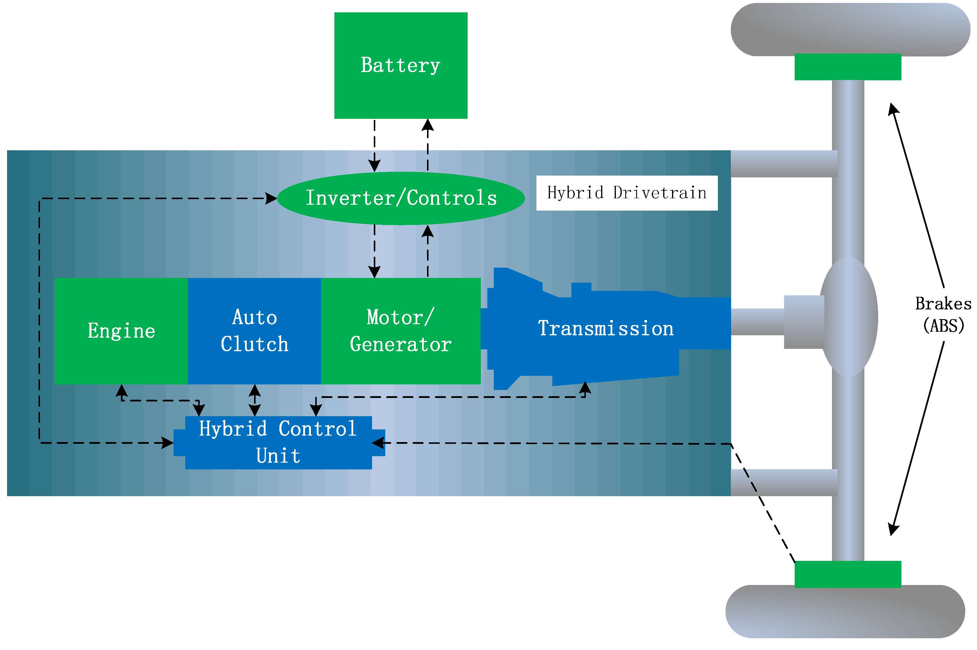
2. Problem Formulation

The prototype vehicle is a single axis parallel HEV, and the drivetrain structure of the HEV is shown in Figure 1. The drivetrain is composed of an engine, an electric traction motor/generator, Ni-MH batteries, an automatic clutch, and an automatic/manual transmission system. The motor is directly linked between the auto clutch output and transmission input. This architecture provides the regenerative braking during deceleration and allows an efficient motor assist operation. To provide pure electrical propulsion, the engine can be disconnected from the drivetrain by the automatic clutch. Important parameters of this vehicle are given in Table 1.
Figure 1. Schematic diagram of the parallel hybrid electric vehicle drivetrain.
Energies 08 11167 g001
Table 1. Summary of the hybrid electric vehicle (HEV) parameters.
ItemParameter
Spark ignition (SI) engineDisplacement: 1.0 L
Maximum power: 50 kW at 5700 r/min
Maximum power: 89.5 N·m at 5600 r/min
Permanent magnet motorMaximum power: 10 kW
Maximum torque: 46.5 N·m
Advanced Ni-MH batteryCapacity: 6.5 Ah
Nominal cell voltage: 1.2 V
Total cells: 120
Automated manual transmission5 speed
GR: 2.2791/2.7606/3.5310/5.6175/11.1066
VehicleCurb weight: 1000 kg
The state vector of the HEV system includes three state variables, i.e., X(k) = (Tdem(k), v(k), SOC(k))T, where Tdem(k) stands for required torque at time k, v(k) is the vehicle speed, and SOC(k) represents the remaining charge of the battery at time k. The control vector is U(k) = Te(k), where Te(k) represents the output torque from the engine. The motor output torque Tm(k) can be obtained by subtracting Te(k) from Tdem(k). A torque split control strategy, which defines the best torque split between the engine and the motor, is adopted.
The control strategy goal of the HEV is to find the optimal control strategy that maps the observed states X(k) to the control action U(k) so as to minimize vehicle fuel consumption and emissions along a traveling route [20]. In the meantime, the vehicle drivability and battery health should be satisfied. Mathematically, the control strategy of the HEV can be formulated as an infinite-horizon dynamic optimization problem as follows:
J ( x ) = k = 0 γ k R ( k )
where R(k) is the immediate cost function incurred by U(k) at time k and γ ∈ (0,1) is a discount factor that assures the convergence of the infinite sum of cost function. One of the key benefits of an infinite horizon problem is that the generated control strategy is time-invariant and, thus, can be easily implemented.
The cost function R(k) consists of the sum of the weighted fuel economy, emissions, and SOC, as shown in Equation (2):
R ( k ) = R fuel ( k ) + a 1 R ems ( k ) + a 2 R SOC ( k )

3. Fuzzy Q-Learning (FQL) Mechanism

The schematic diagram of a FQL control strategy is shown in Figure 2. FQL control strategies consists of two parts: i.e., Q*(x,u) estimator network (QEN) and FIS parameters tuning (FPT). A BP neural network as the QEN is used to estimate Q*(x,u). For the fuzzy controller, we choose a Sugeno-type fuzzy controller.
Figure 2. The schematic diagram of fuzzy Q-learning (FQL) control strategy. QEN: Q*(x,u) estimator network; FIS: fuzzy inference system; AEM: action exploration modifier.
Energies 08 11167 g002

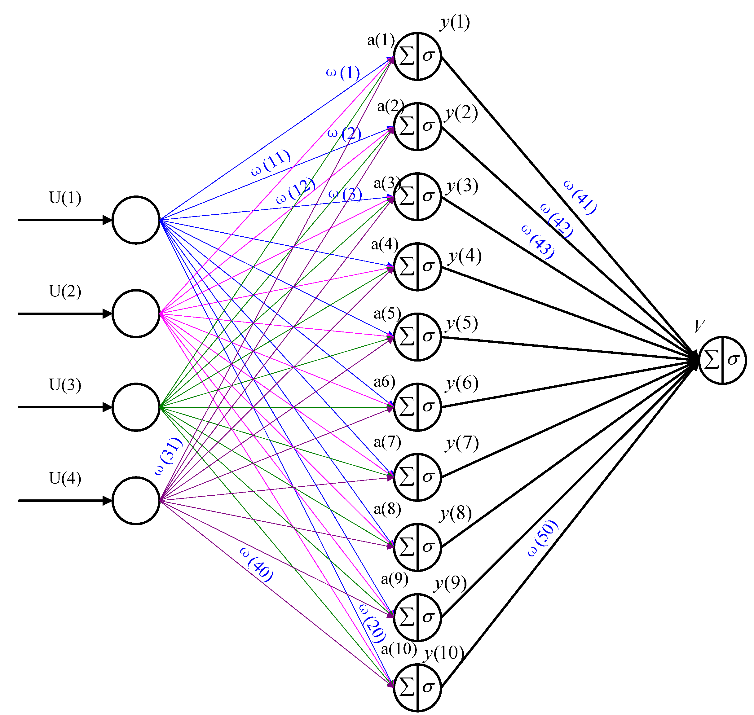
3.1. Back Propagation (BP) Neural Network for Estimating Q*(x,u) (QEN)

The application of reinforcement learning in control problems focuses on two main types of algorithms: actor-critic learning and Q-learning. The actor-critical learning system is a two-step process: i.e. to estimate the state value function J(x) and to choose the optimal action for each state. For Q-learning, the system estimates an action value function Q(x,u) for all state-action pairs and selects the optimal control algorithm based on Q(x,u) [21].
The action value function Q(x,u) is the expected discounted sum of rewards with the initial state x and initial action u which can be written as:
Q ( x , u ) = E { k = 0 γ k r t + k + 1 | x t = x , u t = u }
where u is the action that acts on the system, and E( ) is the expected value function. The optimal action-value function Q*(x,u) is represented as:
Q * ( x , u ) = E { r ( x t + 1 ) + γ max u Q * ( x t + 1 , u ) | x t = x , u t = u }
The QEN plays the role of approximating or predicting the optimal action-value function Q*(x,u) associated with different input states and control output. A BP neural network is adopted to estimate Q*(x,u) due to its good approximation property. The architecture of the QEN is shown in Figure 3. The topology of the QEN is considered to be a three-layer structure having 4-10-1 nodes. The inputs of QEN are state variables of a HEV, and are vehicle speed v(k), battery SOC, required torque Tdem(k), and control action U(k). The output of QEN is Q(x,u).
Figure 3. Architecture of the QEN.
Energies 08 11167 g003
In the QEN, Q(x,u) is represented by:
Q ( x , u ) = f ( V )
V = i = 1 10 ω ( 40 + i ) y ( i )
y ( i ) = f ( a ( i ) )
a ( i ) = j = 1 4 U ( j ) ω ( j 1 , i )
where,
  • V is the summed input of the output node;
  • ω(40 + i) is the weight between hidden node and the output node;
  • y(i) is the output of the hidden node;
  • a(i) is the summed input of ith hidden node;
  • ω(j − 1,i) is the weight between input node and hidden node;
  • U(i) is the input of QEN; and
  • f is the activation function of the node.
Here, a sigmoid function is adopted as an activation function of the node, i.e., f(x) = 1/[1 + exp(−x)].
The parameters of the QEN are tuned based on generalized policy iteration (GPI). We can approximate the optimal action-value function with the neural network by reducing the TD error δt continuously:
δ t = r t + 1 + γ max u Q ( x t + 1 , u ) Q ( x t , u t )
The objective of the neural network is to minimize the following expression:
E = 1 2 δ t 2
The weight-update rule for the neural-network-based gradient-descent method is given by:
ω ( t + 1 ) = ω ( t ) η E ω
E ω = σ t δ t ω = δ t Q ( x t , u t ) ω
Combining the above two equations, we can obtain:
ω ( t + 1 ) = ω ( t ) + ηδ t Q ( x t , u t ) ω
We can obtain Q ( x t , u t ) ω based on the chain rules for ω( 40 + i ) and ω ( j 1 , i ) :
Q ( x t , u t ) ω ( 40 + i ) = Q ( x t , u t ) V V ω ( 40 + i ) = f ( V ) y ( i ) = y ( i ) Q ( x t , u t ) [ 1 Q ( x t , u t ) ]
( for  i = 1 , , 10 )            
Q ( x t , u t ) ω ( j 1 , i ) = Q ( x t , u t ) V V y ( i ) y ( i ) a ( i ) a ( i ) ω ( j 1 , i ) = f ( V ) y ( i ) ω ( 40 + i ) f ( a ( i ) ) u ( j ) = ω ( 40 + i ) u ( j ) Q ( x t , u t ) [ 1 Q ( x t , u t ) ] y ( i ) [ 1 y ( i ) ]
( for  i = 1 , , 10 j = 1 , , 4 )            
also obtaining Q ( x t , u t ) u :
Q ( x t , u t ) u = Q ( x t , u t ) V i = 1 10 ( V y ( i ) y ( i ) ω ( i ) ω ( i ) u ) = f ( V ) i = 1 10 ( w i ( 1 ) f ( ω ( i ) ) w i , 4 ( 2 ) ) = Q ( x t , u t ) [ 1 Q ( x t , u t ) ] × i = 1 10 ( w i ( 1 ) w i , 4 ( 2 ) y ( i ) [ 1 y ( i ) ] )  ∂ Q ( x t , u t ) u = Q ( x t , u t ) V i = 1 10 ( V y ( i ) y ( i ) a ( i ) a ( i ) u )  = f ( V ) i = 1 10 [ ω ( 40 + i ) f ( a ( 5 ) ) ω ( 30 + i ) ]  = Q ( x t , u t ) [ 1 Q ( x t , u t ) ] × i = 1 10 ( ω ( 40 + i ) ω ( 30 + i ) y ( i ) [ 1 y ( i ) ] )
where the control output of FIS is the fourth input of the neural network.

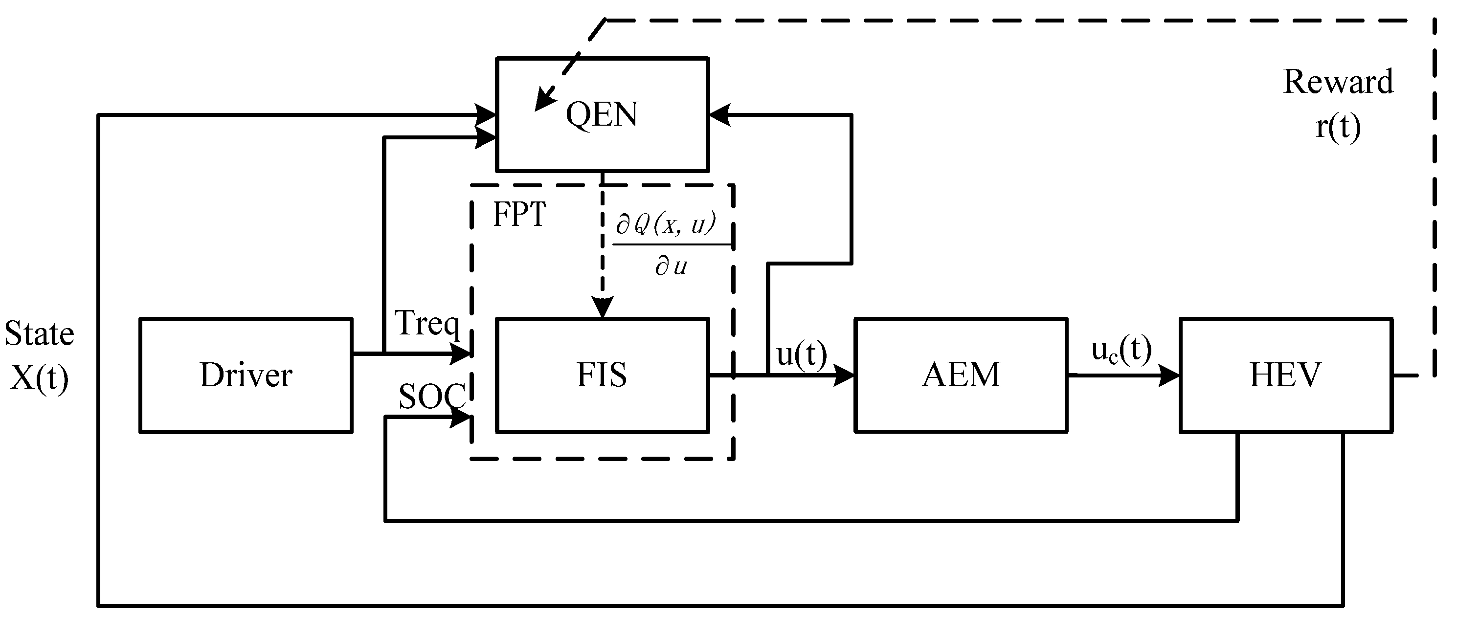
3.2. Fuzzy Interface System (FIS) Parameters Online Tuning-Based on Q*(x,u) (FPT)

This section focuses on how to tune the parameters of the fuzzy controller based on the approximated Q(x,u) obtained from the previous section. In order to optimize the output of the FIS, update the parameters of the FIS to maximize the action value function Q(x,u) with respect to the control output u for the current state. We can tune the parameters of FIS using gradient rules:
ξ ( t + 1 ) = ξ ( t ) + β Q ( x t , u t ) ξ
Q ( x t , u t ) ξ = Q ( x t , u t ) u u ξ
where, ξ is the parameter to be tuned in FIS such as Klj, cli, and δli. We have obtained [ Q ( x t , u t ) ] / u already through Equation (16), thus will only need to deduce u / ξ .
The Sugeno-type fuzzy inference system is chosen in our FQL control strategy. If the state vector is represented by x = ( x 1 , x 2 , ... , x n ) T R n and the control output u R , the IF-THEN rules of the fuzzy controller may be expressed as:
R l : I F x 1 i s F 1 l , ... , a n d x n i s F n l                             T H E N u = K 0 l + K 1 l x 1 + K 2 l x 2 + ... + K n l x n
where Fil is the label of the fuzzy set in xi, for l = 1, 2, …, M. Kl0, Kl1, Kl2,…and Knl are the constant coefficients of the consequent part of the fuzzy rule. We use product inference for the fuzzy implication, singleton fuzzifier, and center-average defuzzifier, respectively. The final output value is:
u ( x _ ) = l = 1 M ( ( i = 1 n μ F i l ( x i ) ) ( j = 0 n K j l x j ) ) l = 1 M ( i = 1 n μ F i l ( x i ) )
where μ F i l is the membership degree of the fuzzy set F i l , x 0 = 1 .
A Gaussian function is used as the membership function of the fuzzy system, i.e.:
μ F i l ( x i ) = e ( x i C i l ) 2 ( σ i l ) 2
for i = 1, 2, …, n ( n is the number of input variable) and l = 1, 2, …, M (M is number of fuzzy rule).
Now we know the parameters that need to be tuned, i.e., c and σ , in our proposed Sugeno-type FIS.
If we let:
z l = i = 1 n exp ( ( x i c i l σ i l ) 2 )
Equation (22) represents the product of different input membership functions in one fuzzy rule:
y ¯ l = K 0 l + K 1 l x 1 + K 2 l x 2 + ... + K n l x n
Equation (23) represents the output of one fuzzy rule:
a = l = 1 M ( y ¯ l z l ) , b = l = 1 M z l , u = a b
where, a, b, and u represents the weighted summation, summation of weight of M rules, and total output respectively.
Thus we can calculate u / ξ by the following equations:
u K j l = z l b x j
u c i l = u z l z l c i l = y ¯ l u b z l 2 ( x i c i l ) ( σ i l ) 2
u σ i l = u z l z l σ i l = y ¯ l u b z l 2 ( x i c i l ) 2 ( σ i l ) 2

3.3. Exploration Policy and Action Modifier

Witkins has shown that Q(x,a) converges to Q*(x,a) with a probability 1, if all actions continue to be tried from all states [22]. In order to guarantee all actions to be tried, we implemented an exploration policy for the control output u recommended by the FIS. The action exploration modifier (AEM) is introduced to generate the control command uc. The uc is the sum of u and an additive disturb action ud, which has a normal distribution with the mean equal to zero and the standard deviation σQ(t) recommended by the FIS. The AEM can solve the dilemma of “exploration” in reinforcement learning, and is added after the FIS and before the system input, i.e., uc = u + ud, and ud ~N(0,σQ(t)).
The σQ(t) calculated as follows:
σ Q ( t ) = k / [ 1 + 2 exp ( max Q ( x , a ) ) ]
where k is coefficient, which can expand or shrink the disturb action.

3.4. Overall Implementation Procedure

The detailed implementation procedure is presented as follows.
1)
Initialize Q(xt,ut), the parameters ω (1)– ω (40), ω (41)– ω (50) of the QEN, and the parameters ξ of the FIS.
2)
Obtain the new control output ut based on (20) and input of the FIS.
3)
Before it is fed to the actual system, u is processed by the action modifier according to uc = u + ud.
4)
The action modifier provides uc, which acts as the control value of the system.
5)
Based on our requirements for the system, we evaluate the performance of the controller as r and obtain the states of the system.
6)
Obtain the approximated Q(xt+1, ut+1) from the QEN based on the current control action, and current states, and some previous states.
7)
From r , Q(xt,ut), and Q(xt+1, ut+1), we can calculate the TD error δt based on Equation (11). Here, we assume Q(xt+1, ut+1) ≈ maxuQ(xt+1, u’) because ut+1 is obtained from the FIS, which continuously maximizes Q(xt,ut) with respect to the control output u .
8)
Based on δt obtained from Step 7, we can update the parameters of the QEN according to Equations (14) and (15).
9)
Tune the parameters of the FIS based on Equations (17)–(27).
10)
Substitute Q ( x t , u t ) with Q ( x t + 1 , u t + 1 ) .
11)
If the parameters of the QEN and the FIS are not changed any more or after predefined iterations, the learning procedure is terminated; otherwise, return to Step 2 after a fixed sampling time Δ .

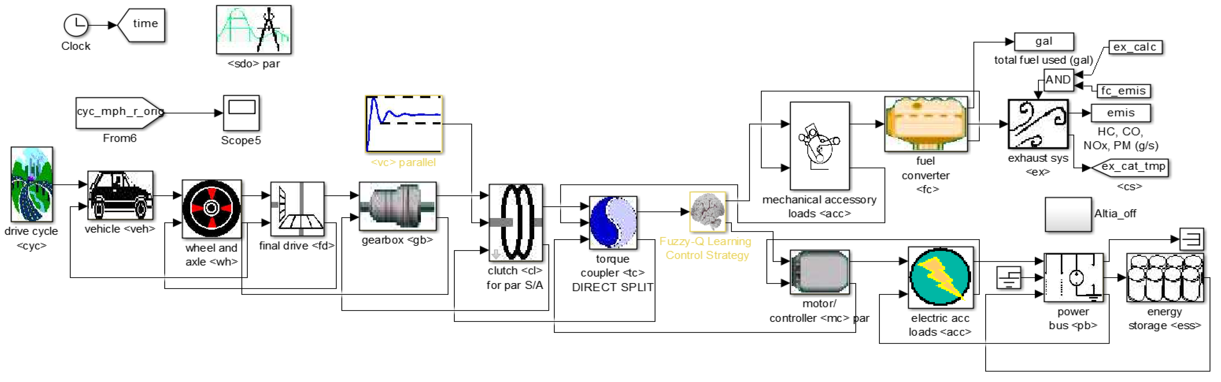
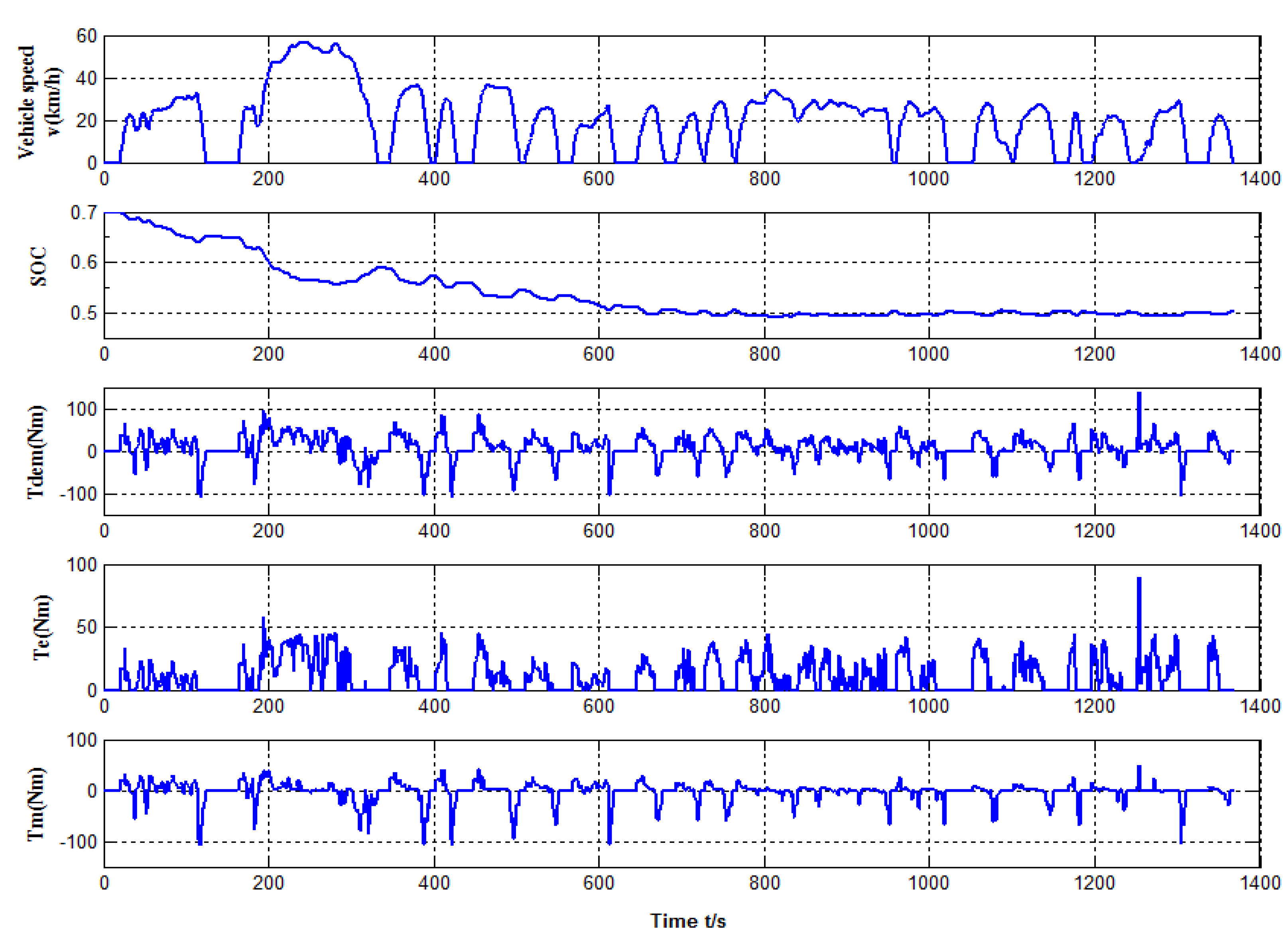
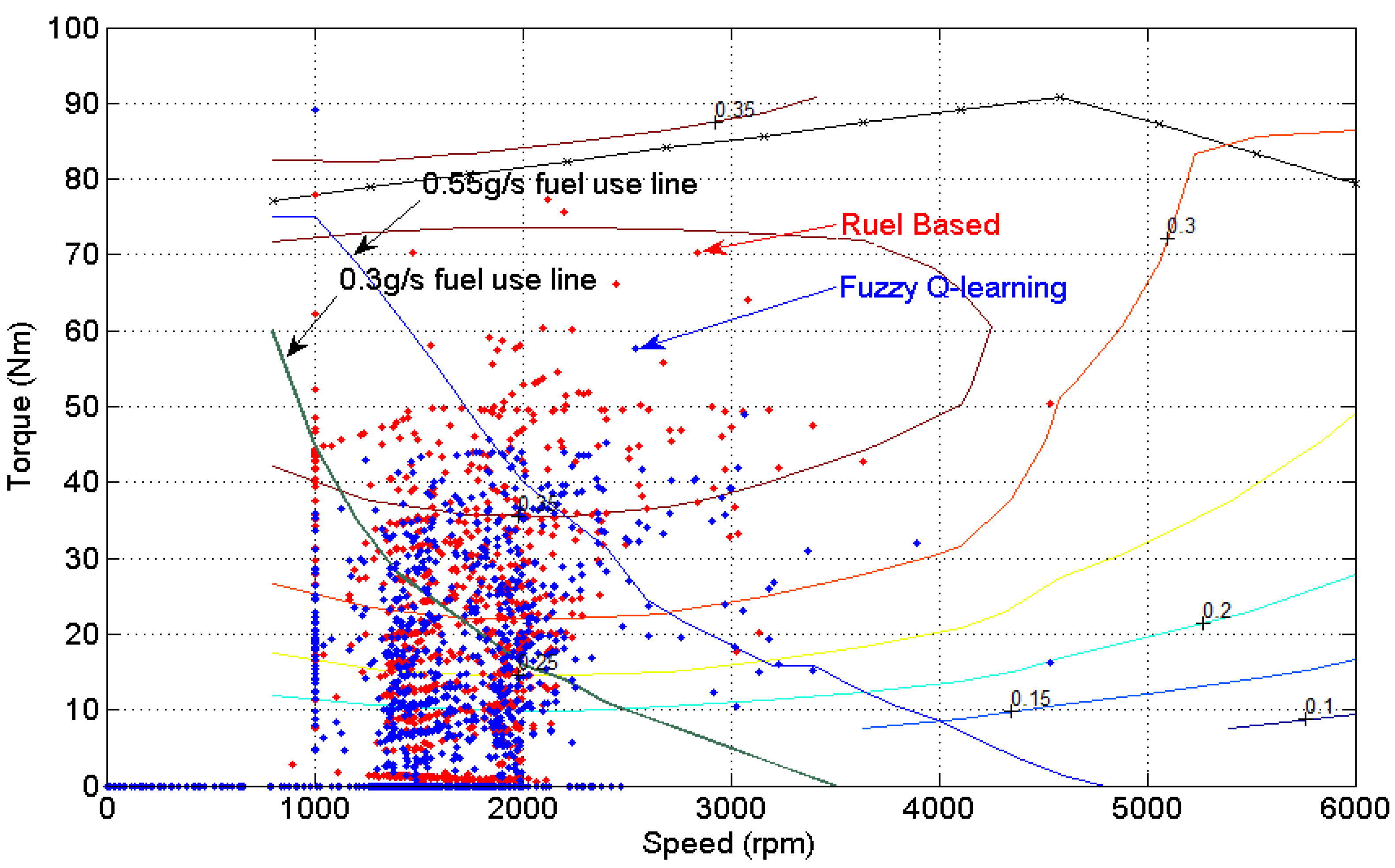
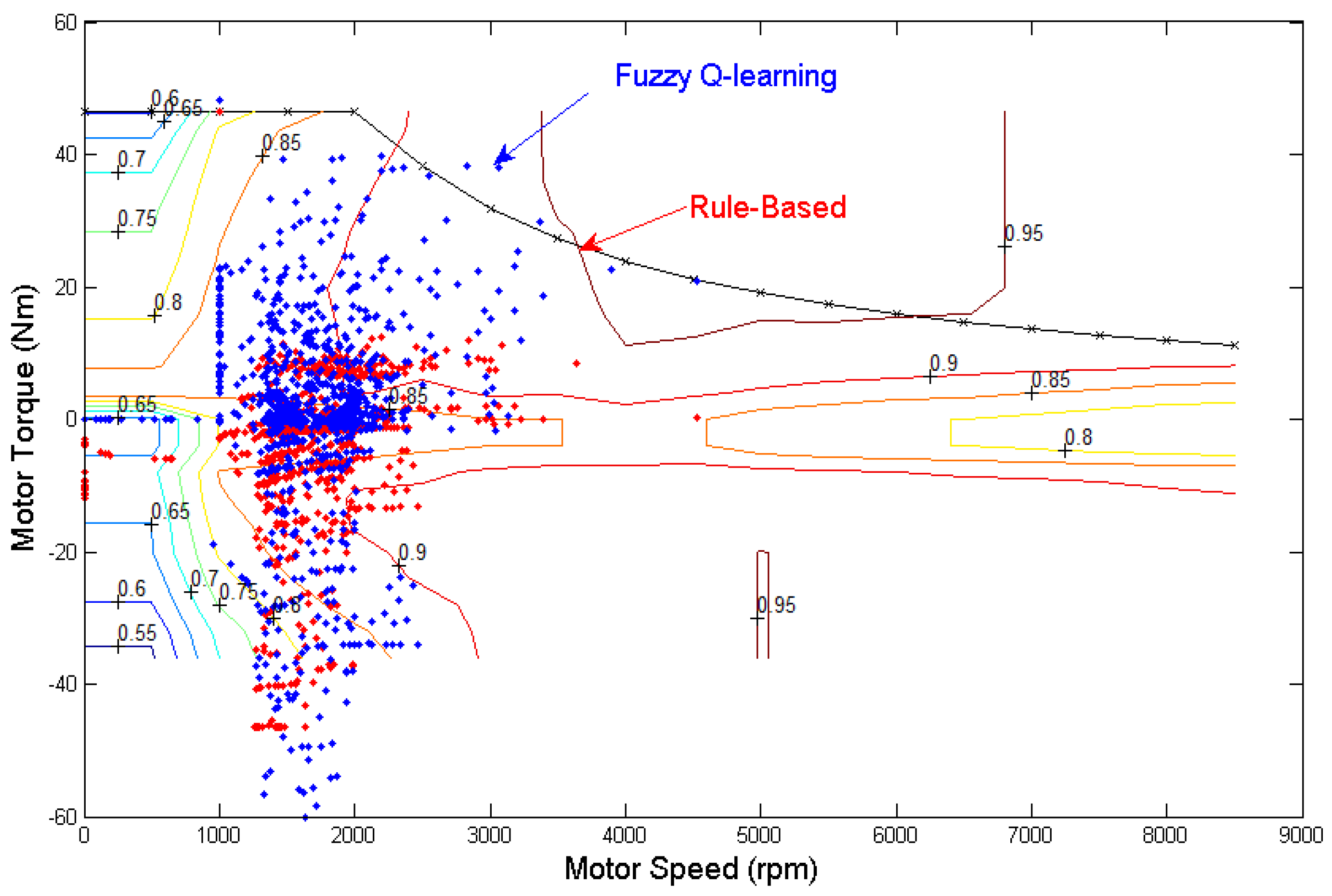
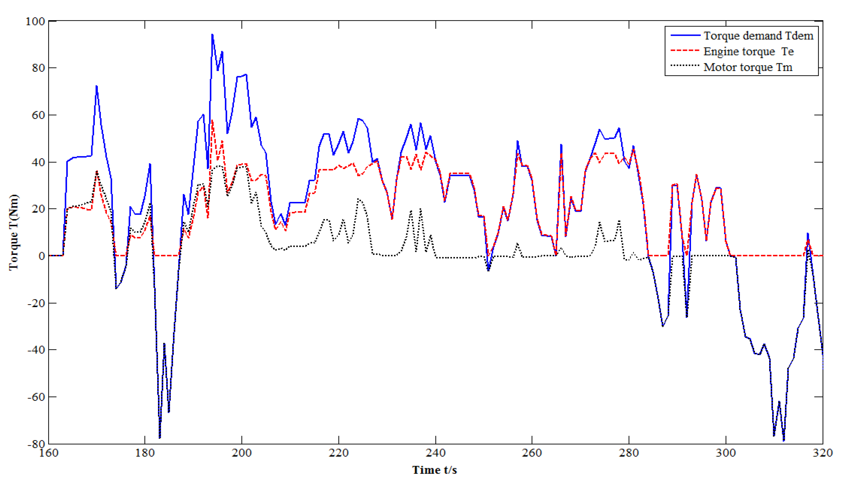
4. Simulation Results and Discussion

In order to know the effectiveness of the FQL algorithm, simulation experiments were done in ADVISOR. Using a simulation to test the algorithm in a variety of driving cycles can eliminate the huge cost and time needed for actual experimentation. The simulation model for the HEV mentioned in section 2 was built in ADVISOR and is shown in Figure 4.
Figure 4. HEV model in ADVISOR.
Energies 08 11167 g004
For this particular HEV system, the parameters of the algorithm used in the simulations are summarized in Table 2, with proper notations defined in it.
Table 2. Summary of FQL algorithm parameters.
ParameterValue
Number of input nodes in QEN4
Number of hidden nodes in QEN10
Learning rate of QEN η0.34
Rate of Gradient descent β0.32
Coefficient of AEM h 0.40
Discount factor γ0.90
Emission cost weight a10
SOC deviation cost weight a21
Coefficient of σQ(t) k 0.41
The next step is to define cost function R(k). The reason for the selection of a1 = 0 is simply because the emission maps are not provided for the engine. Thus, the resultant control strategy is a fuel-economy only strategy. In order to consider the power economy influence on fuel economy, we let a2 equals 1:
R ( k ) = R fuel ( k ) + a 1 R ems ( k ) + a 2 R SOC ( k )
R fuel ( k ) and R SOC ( k ) can be defined as follows:
R fuel ( k ) = { 1 , x > 0.88 g / s ,   0.5 , 0.53 g / s < x < 0.88 g / s , 0.5 , 0 < x < 0.53 g / s .
R SOC ( k ) = { 0.3 , y < 0 ,      0 , 0 < y < 0.001 ,      0.3 , y > 0.001.
where x is the instantaneous fuel consumption value and y the SOC change rate.
The FQL algorithm was written in MATLAB. The fuzzy rules were predesigned according to engineering experience, and complete rules details are given in Table 3, where the parameter of T e satisfies the relationship: VS < S < M < B < VB < SC < MC < BC, the parameters of Tdem and SOC satisfy the relationship: VS < S < M < B < VB.
Table 3. Summary of fuzzy rules.
TeTdem
VSSMBVB
SOCVSBCBCMCSCVB
SBCMCMCSCVB
MSCSCMMB
BSSMBB
VBVSVSSSM
Initially, the membership functions of the fuzzy controller were randomly initialized. In order to illustrate the control strategy more clearly, a convenient method is applied to represent it in an intuitive manner. A torque-split-ratio (TSR) τ = T e / T dem is defined to quantify the positive power flows in the powertrain [23]. Four positive power operation modes are defined, including motor only τ = 0 ), engine only ( τ = 1 ), power-assist ( 0 < τ < 1 ), and charging mode ( τ > 1 ). Figure 5 and Figure 6 show the initial membership functions and TSR map for initial fuzzy controller.
Figure 5. (a) Initial membership functions of T dem ; and (b) initial membership functions of SOC.
Energies 08 11167 g005
Figure 6. Torque-split-ratio (TSR) map for the initial fuzzy controller.
Energies 08 11167 g006
A. Simulation under Urban Dynamometer Driving Schedule (UDDS)
Simulation test was done under standard driving cycle UDDS. Figure 7 depicts the changing trend of the TSR map for fuzzy controller during the driving cycle. From 0 s to 1369 s, we can see that the surface of the TSR map is becoming smoother. The online learning of the fuzzy Q learning control strategy is the reason behind the TSR map smoothing. Figure 8 shows the final membership functions of the fuzzy controller.
Figure 7. Changing trend of fuzzy controller TSR map under Urban Dynamometer Driving Schedule (UDDS): (a) TSR map for fuzzy controller in 500 s; (b) TSR map for fuzzy controller in 1000 s; and (c) TSR map for fuzzy controller in 1369 s.
Energies 08 11167 g007
Figure 8. (a) Final membership functions of T dem under UDDS; and (b) initial membership functions of SOC under UDDS.
Energies 08 11167 g008
The simulation results for the UDDS driving cycles are shown in Figure 9. The FQL control strategy tends to maintain the battery SOC near 50%, finally. This leaves enough capacity to handle an extended period of battery discharge and enough capacity to absorb a long period of charging.
Figure 9. Simulation results under UDDS.
Energies 08 11167 g009
In order to evaluate the performance and effectiveness of the FQL control strategy, the experiment results are compared with a heuristic rule-based control strategy known as “Parallel Electric Assist Control Strategy” and the fuzzy logic control strategy. The comparison results are listed in Table 4. Power consumption is converted to fuel consumption; equivalent fuel consumption is obtained by adding the converted power consumption and fuel consumption. As shown by the results of Table 4, equivalent fuel consumption of fuzzy control is decreased by 3.10% compared with the rule-based control strategy. Meanwhile, the equivalent fuel consumption of the FQL is decreased by 2.67% compared with the fuzzy control strategy. The FQL control strategy achieves good performance.
Table 4. Compare results under UDDS.
Control strategyFuel consumptionEquivalent fuel consumption
Rule-based (L/100 km)3.883.87
Fuzzy control (L/100 km)3.673.75
FQL (L/100 km)3.483.65
Figure 10 and Figure 11 depict the distribution of engine and motor operating points under the rule-based control strategy and FQL control strategy. The FQL control strategy is a fuel strategy which limits the instantaneous fuel consumption. This strategy is not based on the efficiency of the engine, but it primarily limits the fuel use to a particular value. As shown in Figure 10, most of the engine operation points under the FQL control strategy are below the 0.3 g/s fuel use line, while a great amount of engine operation points under the rule-based control strategy are below the 0.55 g/s fuel use line. That means the instantaneous fuel consumption of the FQL control strategy is less than the rule-based control strategy most of the time. The motor operation point distribution of the FQL control strategy is shown in Figure 11. The efficiency of motor operating under the FQL control strategy is better than the rule-based control strategy.
Figure 10. Engine operation point distribution under UDDS.
Energies 08 11167 g010
Figure 11. Motor operation point distribution under UDDS.
Energies 08 11167 g011
Torque split trajectory by using the FQL control strategy is shown in Figure 12. In order to illustrate the torque split trajectory, we choose 160–320 s period from the driving cycle. It is illustrated that the engine provides most of the torque demand, while the motor helps when more torque is needed. The figure also depicts a relatively smooth profile of the engine torque compared with the demand torque and the motor torque. The smoother engine torque from the fuzzy Q learning control strategy indicates that it helps improve the operating conditions of the engine.
Figure 12. Torque split trajectory by using the FQL control strategy under UDDS.
Energies 08 11167 g012
B. Simulation under New European Driving Cycle (NEDC)
In order to check the effectiveness of the proposed method, it is tested on different driving conditions (NEDC driving cycles) starting from the same initial conditions (the same parameters for both neural network and fuzzy controller). Figure 13 show the final membership functions of the FQL control strategy under NEDC cycle are different from that under UDDS cycle; as a result we get two different controllers. That is, the control strategy really learns from the environment.
Figure 13. (a) Final membership functions of Tdem under New European Driving Cycle (NEDC); (b) Initial membership functions of SOC under NEDC.
Energies 08 11167 g013
Simulation results for the NEDC driving cycles are shown in Figure 14. We can see that the SOC also maintains near 50%, finally. The rules of the fuzzy controller have a significant effect on the final value of SOC to make sure that SOC is maintained near 50%, and the proposed method in this paper only changes the parameters of the membership function of the fuzzy controller during the cycle. Table 5 shows the comparison between fuel consumption and equivalent fuel consumption with different control strategies, and we can see the FQL control strategy also achieves good performance.
Figure 14. Simulation results under NEDC.
Energies 08 11167 g014
Table 5. Compare results under NEDC.
Control strategyFuel consumptionEquivalent fuel consumption
Rule-based (L/100 km)3.903.92
Fuzzy control (L/100 km)3.673.79
FQL (L/100 km)3.433.66

5. Conclusions

An online learning control strategy based on FQL has been proposed to improve the fuel economy for a hybrid electric vehicle. The FQL control strategy contains two parts: QEN and FPT. We used a BP neural network as QEN to estimate Q*(x,u). For the fuzzy controller, we chose a Sugeno-type fuzzy controller and the parameters of the fuzzy controller were tuned online based on Q*(x,u). The action exploration modifier (AEM) is introduced to guarantee all actions are tried. Simulation results indicate that the parameters of the FIS are tuned online and the FQL control strategy achieves good performance in fuel economy.

Acknowledgments

This research is supported by National Natural Science Foundation of China (61273139), Natural Science Foundation of Shandong (ZR2014FP001).

Author Contributions

Yue Hu designed the FQL control strategy in matlab and wrote the main parts of the manuscript. Weimin Li proposed the method of FQL control strategy and checked the whole manuscript. Hui Xu did simulation experiments and wrote the part of Simulation results and discussion. Guoqin Xu checked the results and the whole manuscript.

Conflicts of Interest

The authors declare no conflict of interest.

References

  1. Pisu, P.; Rizzoni, G. A comparative study of supervisory control strategies for hybrid electric vehicles. IEEE Trans. Control Syst. Technol. 2007, 15, 506–518. [Google Scholar] [CrossRef]
  2. Wirasingha, S.G.; Emadi, A. Classification and review of control strategies for plug-in hybrid electric vehicles. IEEE Trans. Veh. Technol. 2011, 60, 111–122. [Google Scholar] [CrossRef]
  3. Li, C.; Liu, G. Optimal fuzzy power control and management of fuel cell/battery hybrid vehicles. J. Power Sources 2009, 192, 525–533. [Google Scholar] [CrossRef]
  4. Odeim, F.; Roes, J.; Lars, W.; Angelika, H. Power management optimization of fuel cell/battery hybrid vehicles with experimental validation. J. Power Sources 2014, 252, 333–343. [Google Scholar] [CrossRef]
  5. Zhang, C.; Vahidi, A.; Pisu, P.; Li, X.; Tennant, K. Role of terrain preview in energy management of hybrid electric vehicles. IEEE Trans. Veh. Technol. 2010, 59, 1139–1147. [Google Scholar] [CrossRef]
  6. Lu, S.; Hillmansen, S.; Roberts, C. A power-management strategy for multiple-unit railroad vehicles. IEEE Trans. Veh. Technol. 2011, 60, 406–420. [Google Scholar] [CrossRef]
  7. Zheng, C.; Chris, C.M.; Xiong, R.; Xu, J.; You, C. Energy management of a power-split plug-in hybrid electric vehicle based on genetic algorithm and quadratic programming. J. Power Sources 2014, 248, 416–426. [Google Scholar]
  8. Zhang, C.; Vahidi, A. Route preview in energy management of plug-in hybrid vehicles. IEEE Trans. Control Systems Technol. 2012, 20, 546–553. [Google Scholar] [CrossRef]
  9. Han, J.; Park, Y.; Kum, D. Optimal adaption of equivalent factor of equivalent consumption minimization strategy for fuel cell hybrid electric vehicles under active state inequality constraints. J. Power Sources 2014, 267, 491–502. [Google Scholar] [CrossRef]
  10. Ansarey, M.; Masoud, S.P.; Hussein, Z.; Mohammad, M. Optimal energy management in a dual-storage fuel-cell hybrid vehicle using multi-dimensional dynamic programming. J. Power Sources 2014, 250, 359–371. [Google Scholar] [CrossRef]
  11. Chen, H.; Wu, G.; Luo, L.; Tan, W. Simulation of hybrid electric vehicle control strategy based on compensation fuzzy neural network. In Proceedings of the 7th Intelligent Control and Automation World Congress, Chongqing, China, 25–27 June 2008; pp. 8697–8701.
  12. Meng, X.; Langlois, N. Optimized fuzzy logic control strategy of hybrid vehicles using ADVISOR. In Proceedings of the IEEE Computer, Mechatronics, Control and Electronic Engineering (CMCE) International Conference, Changchun, China, 24–26 August 2010; pp. 444–447.
  13. Chen, R.; Li, C.; Meng, X.; Yu, Y. The application of fuzzy-neural network on control strategy of hybrid vehicles. In Proceeding of the 27th Chinese Control Conference, Kunming, China, 16–18 July 2008; pp. 281–284.
  14. Bichi, M.; Ripaccioli, G.; Di, C.S.; Bemardini, D.; Bemporad, A.; Kolmanovsky, I.V. Stochastic model predictive control with driver behavior learning for improved powertrain control. In Proceeding of the 49th IEEE Decision and Control Conference, Atlanta, GA, USA, 15–17 December 2010; pp. 6077–6082.
  15. Borhan, H.; Vahidi, A.; Phillips, A.M.; Kuang, M.L.; Kolmanovsky, I.V.; Di, C.S. MPC-based energy management of a power-split hybrid electric vehicle. IEEE Trans. Control Syst. Technol. 2012, 20, 593–603. [Google Scholar] [CrossRef]
  16. Bubna, P.; Brunner, D.; Advani, S.G.; Prasad, A.K. Prediction-based optimal power management in a fuel cell/battery plug-in hybrid vehicle. J. Power Sources 2010, 195, 6699–6708. [Google Scholar] [CrossRef]
  17. Santucci, A.; Sorniotti, A.; Constantina, L. Power split strategies for hybrid energy storage systems for vehicular applications. J. Power Sources 2014, 258, 395–407. [Google Scholar] [CrossRef]
  18. Bordons, C.; Ridao, M.A.; Pérez, A.; Marcos, D. Model predictive control for power management in hybrid fuel cell vehicles. In Proceedings of the IEEE Vehicle Power and Propulsion Conference, Lille, France, 1–3 September 2010; pp. 1–6.
  19. Yan, Y.; Xie, H. Model predictive control for series-parallel plug-in hybrid electrical vehicle using GPS system. In Proceedings of Electrical and Control Engineering International Conference, Yichang, China, 16–18 September 2011; pp. 2334–2337.
  20. Li, W.; Xu, G.; Xu, Y. Online learning control for hybrid electric vehicle. Chin. J. Mech. Eng. 2012, 25, 98–106. [Google Scholar] [CrossRef]
  21. Dai, X.; Li, C.K.; Ahmad, B.R. An approach to tune fuzzy controllers based on reinforcement learning for autonomous vehicle control. IEEE Trans. Intell. Transp. Syst. 2005, 6, 285–293. [Google Scholar] [CrossRef]
  22. Watkins, C. Learning from delayed rewards. Ph.D. Thesis, University of Cambridge, Cambridge, UK, 1989. [Google Scholar]
  23. Lin, C.C.; Peng, H.; Grizzle, J.M.; Kang, J.M. Power management strategy for a parallel hybrid electric truck. IEEE Trans. Control Syst. Technol. 2003, 11, 839–849. [Google Scholar]

