An Energy Management Service for the Smart Office

Abstract

The evolution of the electricity grid towards the smart grid paradigm is fostering the integration of distributed renewable energy sources in smart buildings: a combination of local power generation, battery storage and controllable loads can greatly increase the energetic self-sufficiency of a smart building, enabling it to maximize the self-consumption of photovoltaic electricity and to participate in the energy market, thus taking advantage of time-variable tariffs to achieve economic savings. This paper proposes an energy management infrastructure specifically tailored for a smart office building, which relies on measured data and on forecasting algorithms to predict the future patterns of both local energy generation and power loads. The performance is compared to the optimal energy usage scheduling, which would be obtained assuming the exact knowledge of the future energy production and consumption trends, showing gaps below 10% with respect to the optimum.

1. Introduction

The novel smart grid concept is not only revolutionizing the electricity grid infrastructure, but also incentivizing awareness of a more sustainable energy utilization: “green” solutions for residential and commercial buildings have been investigated with the aim of increasing the diffusion of renewable energy sources and reducing carbon footprints [1,2]. However, the inherently intermittent production patterns of renewables (such as solar and wind energy) increase the unpredictability of the overall power availability, thus raising power balancing issues in the management of the smart grid [3].

Concurrently, the “smart building” paradigm [4,5] aims at improving the energy efficiency and occupant’s quality of living by integrating intelligent control mechanisms enabled by information and communication technologies (ICT). The goal of such systems is the optimization of the building operation by integrating information about the users’ preferences and activities, ambient conditions and electricity supply availability. In particular, demand-response interactions make it possible to equalize the load experienced by the grid by lowering the consumption in the case of power production scarcity or by increasing power absorption when production exceeds demand. To do so, the smart building must include distributed generation plants, storage capabilities and controllable electrical loads in a building-integrated microgrid fashion [6,7,8]. Each smart building can be managed by a dedicated control system, which schedules the charge/discharge cycles of the storage bank and the runtime of the power loads, in case they exhibit some malleability (e.g., deferrable loads, such as the recharge of the batteries of electric vehicles or electronic devices, or tunable loads, such as cooling and heating systems): several management policies have been investigated, mostly aimed at the minimization of the operational costs in the presence of time-variable energy tariffs [9,10].

In our preliminary work [11], we propose a smart office architecture in which the energy usage of an office equipped with a photovoltaic plant, a storage bank and a set of loads (either non-deferrable or deferrable) is controlled by means of an energy manager, which makes decisions based on energy production and consumption forecasting algorithms and exploits the following peculiarities of the smart office ecosystem:

• With respect to residential buildings, in which power consumption usually exhibits peaks in the early morning and during the evenings, in a smart office the production pattern of the photovoltaic plant is better aligned with the peak consumption periods, which usually occur during the day;
• Heating, cooling and lighting consumption can be forecasted according to the utilization schedules of the rooms (e.g., the usage of conference rooms is mostly pre-planned by means of a booking mechanism; the occupation of offices depends on the traveling and time-off patterns of the employees);
• Deferrable loads, such as the battery recharge of laptops and mobile devices, can be planned according to the periods in which the devices are plugged in at the working stations, which can be declared in advance by the device owners according to their daily working schedule.

In this paper, we further expand the discussion of our proposed cloud-based energy management service (EMS), which can be provided by a specialized third party, by the utility or by the distribution system operator (DSO). The EMS defines the amount of charged/discharged energy in/from the local storage bank, the runtime of controllable loads and the amount of energy to be absorbed/injected into the grid based on the electricity tariffs. We also present a novel algorithm by which the EMS can minimize the energy expenses or maximize its ability to work in islanded mode, i.e., without injecting nor absorbing energy into/from the grid. The latter objective could be adopted in case the DSO notifies the EMS of an ongoing emergency (e.g., a high probability of outages due to temporary faults or malfunctions in the power grid), in order to privilege a grid-detached operational regime. To achieve these objectives, the EMS solves a mixed-integer linear program (MILP) at regular intervals, taking as input both the actual energy production/consumption data and forecasts about the future production/consumption patterns. The cloud-based EMS can either make locally-optimal decisions or can exploit its knowledge of other subscriber data and of grid data in order to achieve even better results.

The remainder of the paper is structured as follows: Section 2 provides a brief overview of the related work, whereas Section 3 introduces the general framework of the smart office building, the energy production/consumption forecasting algorithms and the MILP executed by the EMS. Section 4 compares the results obtained by the proposed system to the performance achieved by running the MILP under the assumption of full knowledge of the future energy production/consumption trends. Section 5 concludes the paper.

2. Related Work

Several optimization methods for the energy and comfort management of both residential and commercial smart buildings have been proposed by the scientific community, with strategies ranging from day-ahead to real-time planning (the reader is referred to [12] for a comprehensive survey). They are often based on the users’ behavior profiling with the purpose of inferring the main habits and to automatically act on them to reduce energy dissipation, e.g., by switching off stand-by devices [13,14,15]. The integration of local renewable energy production sources and of storage devices has also been widely addressed (see, e.g., [6,16]). Moreover, various optimization models integrating demand-side management mechanisms for the interaction between the smart building and the electricity grid have been comparatively discussed in the survey paper [17].

A consistent body of recent works has specifically addressed the peculiarities of smart office and smart campus environments. Guan et al. [2] designed a MILP for the minimization of gas and electricity bills of a university campus building equipped with a controllable combined heat-power system, battery storage and a photovoltaic plant. The program is applied both under the assumption of a deterministic scenario or of a “scenario tree”, where uncertainty about future power usage is taken into account by means of a weighted objective function, including various production/consumption patterns, each one occurring with different probabilities. Our approach also uses an MILP, but the deterministic scenario is compared to an optimization method in which the model is solved multiple times during the optimization horizon and scheduling decisions are dynamically updated.

A framework for the power management in a smart campus environment is proposed also by Barbato et al. [18], which enables the integration of renewable local energy sources, storage banks and controllable loads, and supports demand response with the electricity grid operators. The framework includes an energy management system running a linear program to schedule electrical loads based on the forecasted energy production/consumption, on the current energy tariff trend and on the comfort level perceived by the building occupants. Such an optimizer is integrated within an ICT infrastructure, which collects sensor data from the campus buildings and actuates the computed schedules. In our framework, we adopt a similar architectural approach.

A hierarchical multiagent control system for a microgrid-integrated smart building is discussed by Wang et al. [19]. A particle-swarm optimization method is applied by the main agent for the maximization of the user comfort, whereas additional local agents manage controllable loads, room illumination, temperature and air quality by means of fuzzy rules. The operational state of the smart building (grid-connected or islanded) is chosen based on the grid conditions (i.e., presence of disturbances) and on the energy availability from local renewable energy sources. Similarly, in our framework, the smart building preferably operates in islanded mode upon notification of grid faults/malfunctions from the DSO. However, we opted for a MILP as the optimization method with the aim of minimizing the daily electricity bill, rather than maximizing the perceived comfort.

Methods for knowledge extraction to automatically infer and adapt rule sets for the management of a smart office (or a generic smart building) are proposed by Gupta et al. [20] and Anjos et al. [21]. By analyzing data gathered from electricity meters, sensors and actuators deployed within the office environment and combining them with the users’ preferences, control rules can be dynamically generated, modified and deleted. However, this approach does not provide any guarantee of optimality.

Real testbeds deployed in office buildings aimed at the development of self-sustained distributed energy systems are described in [22,23,24]. The results presented in this paper have been obtained based on data provided by the “Smart Energy Living Lab” located at the fortiss premises [24].

3. The Smart Office Environment

The fortiss Smart Energy Living Lab is envisioned as an example of the adaptive control and responsive behavior of a smart building. Based on the current and predicted generation of renewable energy and on the available storage capacity, it is possible to control office appliances in order to achieve a better utilization of energy. Imagine a sunny day, which leads to an overproduction of the solar energy generation. Once the batteries of the storage bank are fully charged, the surplus could be used to cool down the server room more than usual. Hence, the server room has not to be cooled down for a longer period of time. Alternatively, taking the current energy prices into account, the excess energy can be fed into the network to achieve an economic profit. In the following, we will summarize the general framework of the fortiss Smart Energy Living Lab [25] before explaining the components and algorithms used to predict the future energy generation/consumption and to schedule the smart building operations.

3.1. General Framework

For the Smart Energy Living Lab, a flexible, extensible and lightweight architecture is used, which follows a layered and component-based approach to ensure scalability, flexibility and extensibility. An overview of the system is illustrated in Figure 1. Starting at the bottom, several sensors and actuators are connected to the server application, or middleware, respectively. The sensor and actuator layer of the middleware support different protocols, like IEC61850 via Modbus, ZigBee, and EnOcean, to exchange information and control signals with different sensors and actuators from both the home automation and the energy domain. This enables the system to provide monitoring and control capabilities for the photovoltaic installation, the backup batteries, air condition, blinds, lights, power plugs, window sensors, humidity, temperature, brightness and power meters. For additional details regarding the system middleware, the reader is referred to [24].

Figure 1. Overview of the Smart Energy Living Lab.

Figure 1. Overview of the Smart Energy Living Lab.

Software components within the system layer of the server application enable the management of users, their roles, associations with rooms and personal profiles, as well as the modeling of smart building environments in terms of assigning devices to rooms and these to floors or buildings, respectively. This layer includes a central registrar to enable the integration of additional sensors and actuators in a plug and play manner. Measured data and control capabilities are available via a REST or WebSocket API on different devices and clients, and all information is stored in, or retrieved from, a database. In addition, a rule system at the application layer of the middleware is used to observe the current status and under appropriate conditions to issue commands, e.g., to maintain a defined brightness level. Nevertheless, a detailed description of the rule system and of the components dedicated to the extraction of knowledge out of historical data is out of scope of this work.

The server application also manages the interface to the cloud-based EMS, which is accessible via a web service API. Every time epoch, the server application collects the state of charge of the storage devices, the set of devices that can be managed and pushes them to the EMS along with the configuration requests, such as the minimum recharge level that must be guaranteed to the users of the rechargeable devices. The server application also asks the EMS for the load schedule to be applied in the next time epoch.

The EMS performs the optimization and elaborates the load scheduling for the next epochs, which the server application fetches when ready. In our experience, a standard server can optimize the needs of a single smart office in a few seconds, so the server application can receive the answer with very limited latency. Then, the application server enforces the decisions of the EMS by translating them into hard limits on the charge/discharge rate of the battery and on the consumption of deferrable or malleable loads.

Since the EMS makes decisions by using predictions of the consumed/produced power, the server application must also ensure that the EMS decisions are feasible and do not result in unwanted outages if the prediction error happens to be large. This is especially important when the smart office operates in islanded mode: the server application is responsible of early termination of the islanded mode if the consumption exceeds the available power from the photovoltaic plant plus the storage bank.

Employing a cloud-based EMS rather than an on-premises solution is a fundamental design choice of our framework, which enables the implementation of advanced services.

Cloud-based energy monitoring systems are increasingly popular, because of their ease of deployment, faster time-to-repair and reduced costs thanks to infrastructure sharing with several customers, resulting in economies of scale. In addition to these advantages, a cloud-based decision system, such as our EMS, can also yield better decisions by exploiting information from other users in the same area or from the grid operator itself and could also coordinate the decisions of multiple entities.

In particular, we assume that the EMS autonomously collects any additional data necessary for the optimization, such as the energy purchasing and selling prices in the next epochs, the production forecast for the subscriber’s photovoltaic plant, the consumption forecast, etc. If the EMS is provided by a grid operator, it also receives any requests from the grid to cap the power bought or sold, or even to enter islanded operation.

There are a few issues that must be considered before deploying a cloud-based solution. The first issue is that network connectivity issues make the EMS unreachable and, thus, unable to manage the devices. We observe that many offices nowadays are moving towards cloud-based solutions for their mission-critical systems, such as management software or productivity suites. As a consequence, businesses generally have high availability contracts with Internet service providers and backup solutions. The second major issue is that a centrally-managed EMS leaks private information about the ongoing or scheduled activities in the office. To this end, there is a rich research area discussing how to perform privacy-preserving energy scheduling at the expense of an increase of computation effort [26] or of potential savings [27].

3.2. Energy Production and Consumption Forecast Algorithms

For the determination of optimized schedules to achieve economic savings taking into account load shifting and variable energy tariffs, forecasts of both the local energy generation and consumption are essential. In this work, the forecasts are generated at midnight for the next 24 h with a granularity of 15-min intervals.

3.2.1. Generation Forecast

The generation forecast utilizes the OpenWeatherMap API [28], which provides weather forecasts for three hour-long periods. Available information includes sunrise and sunset times, a weather condition code and the percentage of sky coverage due to clouds. The weather condition code $\gamma \left(t\right)$ (e.g., clear sky, scattered clouds or moderate rain) and the percentage of sky coverage ϕ form a weather factor $\omega \left(t\right)=\gamma \left(t\right)/2+\varphi \left(t\right)/2$ in the range $[0,\dots ,1]$ (with zero being heavy rain and one being clear sky). Before sunrise and after sunset, the generation forecast $G_{\text{fc}}$ is zero; otherwise, it is calculated as follows:

$$G_{\text{fc}}\left(t\right)=\omega \left(t\right)P_{\text{peak}}\left(m\right)·min(exp(-0.3t^2),0.5exp(-0.75t^2))$$

(1)

where the coefficient $P_{\text{peak}}\left(\delta \right)$ indicates the peak production of the installed photovoltaic plant, which varies depending on the time of the year, δ. Several models have been proposed to compute $P_{\text{peak}}\left(\delta \right)$ (see, e.g., [29,30]). In this paper, for the sake of simplicity, we assume a parabolic dependency on the month m (months are numbered $-6\le m\le 5$, with $m=0$ being July) according to the following formula:

$$P_{\text{peak}}\left(m\right)=-75m^2+P{V}_{\text{peak}}\left[W\right]$$

Figure 2 illustrates the results of the actual (solid, blue) and predicted (dashed, green) generation.

Figure 2. Comparison of actual and predicted production

Figure 2. Comparison of actual and predicted production

3.2.2. Consumption Forecast

We applied a triple exponential smoothing model provided by OpenForecast [31] to predict the power consumption, since seasonal models are supposed to be a simple but feasible approach for short-term electricity demand [32,33]. Adequate results have been obtained using a triple exponential smoothing model with parameters (0.7, 0.1, 0.2), which correspond to the weight of recent data, trend and seasonality, respectively. The basis for these models are time series, where we use the historical consumption data for the past six same days (either working or high days). If we utilized information from the last successive days, the strong differences between workdays and weekends would distort the forecast values. Figure 3 illustrates the results of the actual (solid, blue) and predicted (dashed, green) consumption, where the difference in the power demand of workdays and the weekends becomes evident.

Additional calendar information regarding the booking of the conference rooms, including the expected participants and the type of the meeting, is also integrated into the forecasting algorithm. In our approach, we subtract the consumption of the respective conference rooms, which are also monitored, from the overall consumption used for the described demand forecast. Then, predefined consumption profiles for each conference room are added to the calculated forecast for the period of the reservations of the corresponding room, e.g., when it is booked for a presentation from 15:00 until 17:00.

Figure 3. Comparison of actual and predicted consumption.

Figure 3. Comparison of actual and predicted consumption.

3.3. The Energy Manager

The energy management algorithm assumes that the optimization horizon is divided into a set of epochs $\mathcal{T}$ of fixed duration (e.g., in the order of minutes) and works under the following assumptions:

• The battery of the local storage bank can be charged (possibly with interruptions) with the energy generated by the photovoltaic plant and/or by direct feeding from the electricity grid;
• No more energy than the daily production of the photovoltaic plant can be injected into the grid (this prevents the smart office from getting state incentives for reselling energy bought from the grid);
• The duration of plug-in periods of rechargeable electronic devices is specified by the owners at the moment of plugging in the device. Alternatively, these periods could be enforced by using switchable sockets controlled by the system. The recharge process can possibly experience intermediate interruptions. Recharge is mandatory if the current state of charge of the device battery is below a given threshold specified by the user.

Whenever a new epoch t starts, the energy manager receives the energy production/consumption forecasts computed by the algorithms presented in Section 3.2, the actual amounts of energy generated and consumed in the previous epochs $1,\cdots ,t-1$, the current state of charge of the storage bank and of the batteries of the electronic devices actually plugged in for recharge. The expected plug-in periods of the electronic devices can be either computed according to the historical data or to the office usage schedule. The energy manager then runs an MILP to schedule the energy usage for the current epoch, which is defined as follows.

3.3.1. Sets

• $\mathcal{T}=\{t,\cdots ,T\}$: Set of time epochs within the optimization temporal horizon
• $\mathcal{J}$: Set of rechargeable devices

3.3.2. Parameters

• $p_i$: Forecasted energy production of the photovoltaic plant for epochs $i\in \mathcal{T}$;
• $c_i$: Forecasted energy consumption of non-deferrable loads for epochs $i\in \mathcal{T}$;
• $e{p}_i/e{s}_i$: Energy purchasing/selling price for epochs $i\in \mathcal{T}$ (note that the energy tariff can be either known in advance or dynamically adjusted: in the latter case, energy prices are forecasted according to historical knowledge and then updated epoch by epoch according to the actual values);
• B: Actual state of charge of the storage bank at the end of epoch $t-1$;
• L: Storage bank capacity;
• R: Maximum charge/discharge rate of the storage bank;
• Forecasted/actual plug-in periods ($w_i^j$), initial state of charge ($B{w}^j$), battery recharge rate ($R{w}^j$), minimum recharge level ($M{w}^j$) and capacity ($L{w}^j$) of each rechargeable device j, for epochs $i\in \mathcal{T}$. It must hold that $M{w}^j\ge B{w}^j$;
• $r_i^j$: Reward for recharge of device j at epochs $i\in \mathcal{T}$;
• ${\Pi }^p/{\Pi }^s$: Contractual upper limit to the power amount absorbed/injected into the grid during one epoch;
• $I_i$: Binary parameter, set to one if the islanded operational mode during epoch $i\in \mathcal{T}$ is preferable (e.g., due to critical grid conditions), zero otherwise;

3.3.3. Variables

• $x_i^c,x_i^d$: Binary variables, set to one if the storage bank is charged/discharged during epochs $i\in \mathcal{T}$, to zero otherwise;
• $y_i^p,y_i^s$: Non-negative variables indicating the amount of purchased/sold energy during epochs $i\in \mathcal{T}$;
• $z_i^j$: Binary variables indicating the schedule of the recharge periods of each electronic device j during epochs $i\in \mathcal{T}$ (not in charge = 0, in charge = 1);
• $b_i^c,b_i^d$: Non-negative variables defining the amount of energy charged/discharged into/from the battery during epochs $i\in \mathcal{T}$;
• ${\alpha }_i$: Binary variables set to one if the smart office operates in islanded mode during epochs $i\in \mathcal{T}$, to zero otherwise;
• $h_i$: Binary variables set to one if the smart office switches from islanded to grid-connected mode during epochs $i\in \mathcal{T}$, to zero otherwise;
• $s_i$: Non-negative variables indicating the energy surpluses generated by the photovoltaic plant during epochs $i\in \mathcal{T}$ when operating in islanded mode.

3.3.4. Objective Functions

The first objective function (Equation (2)) minimizes a weighted sum of two contributions, i.e., operational costs (in terms of daily energy expenses) and rewards for the recharge of the batteries of the electronic devices above the minimal threshold. Rewards are design parameters that can be adjusted to privilege one or the other objective. Alternatively, the second objective function (Equation (3)) maximizes the number of epochs in which the smart office operates in islanded mode while minimizing the amount of energy wastage due to production surpluses. Equation (2) is used by default and can be substituted by Equation (3) in case the DSO notifies that there is an emergency period (due to an overload, a fault or a malfunction of the grid), in order to privilege the islanded operational regime. In such a case, the energy manager is responsible for replacing Equation (2) with Equation (3) upon emergency notification from the DSO.

$$min\sum _{i\in \mathcal{T}}(y_i^{p}e{p}_i-y_i^{s}e{s}_i)-\sum _{j\in J}(B{w}^j+\sum _{i\in \mathcal{T}}{z}_i^{j}R{w}^j-M{w}^j)r_i^j$$

(2)

$$max\sum _{i\in \mathcal{T}}({\alpha }_i-s_i)$$

(3)

3.3.5. Constraints

Constraint Equations (4) and (5) impose that the amount of absorbed/injected energy does not exceed the contractual limits, when the smart office operates in grid-connected mode, whereas they are forced to be zero when operating in the islanded regime. Equation (6) ensures the balancing of the energy flows (both from/to the grid and from/to the storage bank). The storage bank capacity limits are imposed by constraint Equations (7) and (8), whereas Equation (9) imposes that the battery charge level at the end of the scheduling horizon equals the initial charge level (i.e., B). Similar constraint Equations (10) and (11) are imposed to control the level of the batteries of rechargeable devices. Moreover, constraint Equation (12) restricts the set of epochs during which the electronic devices may be recharged to plug-in periods. Constraint Equation (13) ensures that no more energy is injected into the grid than the amount produced by the photovoltaic plant, whereas constraint Equations (14) to (16) impose that during each epoch, the storage bank is either charged or discharged and prevents the amount of energy charged/discharged into/from the storage bank during each epoch from exceeding the limit imposed by the maximum charge/discharge rate. Constraint Equation (17) limits the periods of the islanded regime to the emergency periods defined by the DSO. Note that the value of the parameter $I_i$ is set to zero when the objective function Equation (2) is used, whereas in the case of emergency notification (i.e., when the objective function Equation (3) is used), its value is provided as input to the energy manager by the DSO itself and is set to one for all of the epochs falling within the time duration of the emergency state. Finally, constraint Equations (18) and (19) prevent multiple transitions from grid-connected to islanded mode. The latter constraints avoid degenerate solutions in which the operational state switches repeatedly from islanded to grid-connected mode within a short time period in order to partially recharge the battery, which in turn makes it possible to operate again in islanded mode in successive epochs.

$$\begin{array}{cc}\hfill y_i^s& \le {\Pi }^s(1-I_i)\forall i\in \mathcal{T}\hfill \end{array}$$

(4)

$$\begin{array}{cc}\hfill y_i^p& \le {\Pi }^p(1-I_i)\forall i\in \mathcal{T}\hfill \end{array}$$

(5)

$$p_i+y_i^p+b_i^d=s_i+c_i+y_i^s+b_i^c+\sum _{j\in \mathcal{J}}R{w}^j{z}_i^j\forall i\in \mathcal{T}$$

(6)

$$\begin{array}{cc}\hfill B+\sum _{k=t}^i(b_k^c-b_k^d)& \le L\forall i\in \mathcal{T}\hfill \end{array}$$

(7)

$$\begin{array}{cc}\hfill B+\sum _{k=t}^i(b_k^c-b_k^d)& \ge 0\forall i\in \mathcal{T}\hfill \end{array}$$

(8)

$$\begin{array}{cc}\hfill B+\sum _{i\in T}(b_i^c-b_i^d)& =B\hfill \end{array}$$

(9)

$$\begin{array}{cc}\hfill B{w}_j+\sum _{i\in \mathcal{T}}R{w}^j{z}_i^j& \le L{w}^j\forall i\in \mathcal{T},j\in \mathcal{J}\hfill \end{array}$$

(10)

$$\begin{array}{cc}\hfill B{w}_j+\sum _{k=t}^{i}R{w}^j{z}_i^j& \ge M{w}^j\forall i\in \mathcal{T},j\in \mathcal{J}\hfill \end{array}$$

(11)

$$z_i^j\le w_i^j\forall i\in \mathcal{T},j\in \mathcal{J}$$

(12)

$$\sum _{i\in \mathcal{T}}{y}_i^s\le \sum _{i\in \mathcal{T}}{p}_i$$

(13)

$$b_i^c/R\le x_i^c\forall i\in \mathcal{T}$$

(14)

$$b_i^d/R\le x_i^d\forall i\in \mathcal{T}$$

(15)

$$x_i^c+x_i^d\le 1\forall i\in \mathcal{T}$$

(16)

$${\alpha }_i\le I_i\forall i\in \mathcal{T}$$

(17)

$${\alpha }_{i-1}-{\alpha }_i\le h_i\forall i\in \mathcal{T}\backslash \left\{t\right\}$$

(18)

$$\sum _{i\in \mathcal{T}}{h}_i\le 1$$

(19)

After running the MILP optimization, the smart office operational mode, the charge/discharge of the storage bank and the recharge of the batteries of the electronic devices for epoch t are then settled according to the MILP output as follows. If ${\alpha }_t=0$, the island mode switch is set to make the smart office operate in grid-connected mode. Then:

• The switchable socket in which electronic device j is plugged is turned on or off according to the value of $z_t^j$;
• The storage bank is configured to charge or discharge according to the values of the binary variables $x_t^c$ and $x_t^d$. In addition, the battery management system is configured to stop charging or discharging when the energy amount, $b_t^c$ or $b_t^d$, respectively, is reached;

The smart office power balance is maintained by means of the connection to the grid.

Conversely, if ${\alpha }_t=1$, the island mode switch is set to make the smart office operate in islanded mode. Then, the switchable socket in which electronic device j is plugged is turned on or off according on the value of $z_t^j$. In islanded mode, the power balance is ensured by the battery management system. When operating in islanded mode, power production surpluses or deficits may occur at any time, e.g., in the case of significant under-/over-estimations of the power usage/generation by the forecasting algorithms with respect to the actual values. When the battery is full or is charging at the maximum rate R, photovoltaic production must be limited. Various algorithms are proposed in the literature to switch from the usual maximum power point tracking (MPPT) to a limited-power regime (e.g., [34]). Conversely, to counteract the effects of unpredicted energy deficits, we assume the presence of an emergency recovery mechanism that automatically switches the operational mode to grid-connected if either the storage bank charge level drops below a safety threshold or it is discharging at a rate above a safety threshold. Such thresholds can be tuned according to the response time of the switching mechanism, in order to ensure a smooth transition of the operational regime.

At the end of epoch t, the state of charge of the storage bank is updated according to the real energy absorption/injection. The same holds for the battery state of charge of the rechargeable devices. The forecasted plug-in periods are also updated according to the users’ behavior during the current epoch (e.g., in case a device j expected to be plugged in by the beginning of epoch $t+1$ has not actually been plugged, then $w_{t+1}^j$ must be set to zero). Moreover, operational costs are updated according to the exact amount of energy absorbed/injected from/into the grid. The whole process is then repeated at the beginning of each successive time epoch, up to epoch T, similarly to a receding horizon mechanism.

4. Performance Evaluation

To assess the performance of our proposed EMS, we tested it in the fortiss Smart Energy Living Lab. The testbed includes a photovoltaic plant with peak production of 10 kWp, a storage bank with capacity of 10 kWh and recharge rate of 1.2 kW, a set of non-deferrable appliances (lights, heating/cooling systems, servers and desktop computers) and 60 controllable plugs to which 30 laptops (device battery capacity of 55 Wh, recharge rate of 45 W) and 30 mobile phones (device battery capacity of 6 Wh, recharge rate of 3 W) can be connected. Recharge is mandatory until device batteries reach 65% of charge.

The scheduling horizon is a 24-h period divided into 96 epochs of a 15-min duration (though from the theoretical point of view, the duration of an epoch can be arbitrarily defined, most of the state-of-the-art commercialized smart meters use measuring intervals of 15 min). We start considering the minimization of the overall operational costs. The rewards for the recharge of the electronic devices above the mandatory threshold are price incentives corresponding to the daily average electricity price. Note that such incentives do not impact the actual bill, since they appear exclusively in the objective function of the MILP model. The electricity prices vary according to three different tariff types currently applied by an Italian energy provider [35] and reported in Figure 4: The flat tariff imposes a constant price during the whole day; the two-tier tariff applies two different prices according to the time of the day (low price from 00:00 to 07:59 and from 19:00 to 23:59, high price from 08:00 to 18:59); the time-of-use tariff exhibits hourly variations according to the fluctuations of the energy market. Prices for selling energy surpluses by injection into the grid are obtained by multiplying the actual purchase prices by a scaling factor $\beta =0.5$ (i.e., $e{s}_i=\beta e{p}_i$). The initial state of charge of the storage bank is assumed to be $B=L/2$. In our implementation, the MILP model is solved by means of the AMPL/CPLEX [36] solver.

To assess the performance of our proposed framework, we compare the daily bill obtained by running the EMS as described in Section 3.3 to the optimal bill, which would be obtained “a posteriori” by running the EMS at the end of the day (i.e., with full knowledge of the real energy production/consumption patterns), and to the performance of a benchmark scenario, which assumes that the smart office always operates with a fully-charged storage bank, that no power is drained from the storage battery and that the recharge of the electrical appliances starts as soon as they are plugged in, until full recharge (i.e., the EMS does not perform any optimization of the power usage). Note that the running times of the AMPL/CPLEX solver on a standard desktop computer was in the order of tens of seconds in all of the considered instances. Results averaged over several days are reported in Table 1 and show that the bill obtained by the EMS is at most 0.05 € higher than the optimal bill, which would be obtained if the future energy production/consumption patterns were known in advance. Conversely, running the smart office in grid-connected mode without relying on the storage bank capacity nor optimizing the recharge periods of the electronic appliances results on average in a 1.3 € higher bill with respect to the optimum. Therefore, intelligently shaping the consumption curve of deferrable appliances and scheduling the usage of the storage capabilities of the smart office leads to consistent economical savings. Moreover, the limited bill increase with respect to to the optimal scheduling shows that the errors introduced by the forecasting algorithms have a very moderate impact on the daily expenses.

Figure 4. Flat, time of use and two-tier tariff prices.

Figure 4. Flat, time of use and two-tier tariff prices.

Table 1. Performance assessment of the Energy Manager with respect to optimal and benchmark scenarios.

Tariff	Average Daily Bill [€]			Average Gap with Respect to Optimum [€]
	Benchmark	Energy Manager	Optimum	Benchmark	Energy Manager
time-of-use	7.76	6.57	6.52	1.24	0.05
flat	8.26	7.03	6.99	1.17	0.04
two-tier	8.45	7.04	7.00	1.45	0.04

Table 1. Performance assessment of the Energy Manager with respect to optimal and benchmark scenarios.

Tariff	Average Daily Bill [€]			Average Gap with Respect to Optimum [€]
	Benchmark	Energy Manager	Optimum	Benchmark	Energy Manager
time-of-use	7.76	6.57	6.52	1.24	0.05
flat	8.26	7.03	6.99	1.17	0.04
two-tier	8.45	7.04	7.00	1.45	0.04

It is worth noting that the time-of-use tariff leads to the lowest bills when compared to the other tariff options: in this scenario, due to the high variability of the energy prices, which exhibit hourly changes, the benefits of charging the battery during low-price periods and to discharge it when prices are higher become more evident. However, in the case of the time-of-use tariff, the schedules defined by the EMS lead to the highest bill gap with respect to to the optimal ones, since with such a tariff, even small deviations with respect to the optimal schedules, due to inexact forecasts, could result in non-negligible additional expenses.

We now detail the analysis of the numerical results obtained for two reference days (a sunny weekend day and a partially-cloudy working day, respectively), assuming the usage of time-of-use tariffs. The corresponding energy exchanges with the grid obtained by means of the EMS are reported in Figure 5, Figure 6 and Figure 7. The trends depicted in Figure 5 show that during a sunny weekend, the photovoltaic plant generation is sufficient to avoid energy purchases, to recharge the battery storage bank and even to sell production surpluses for most of the daylight time. In order to leave a sufficient capacity to store the power generated by the solar panels, the storage bank is mostly discharged during the early morning. The battery is also discharged during the evening period, in order to reduce the amount of purchased energy when prices are high (see Figure 4).

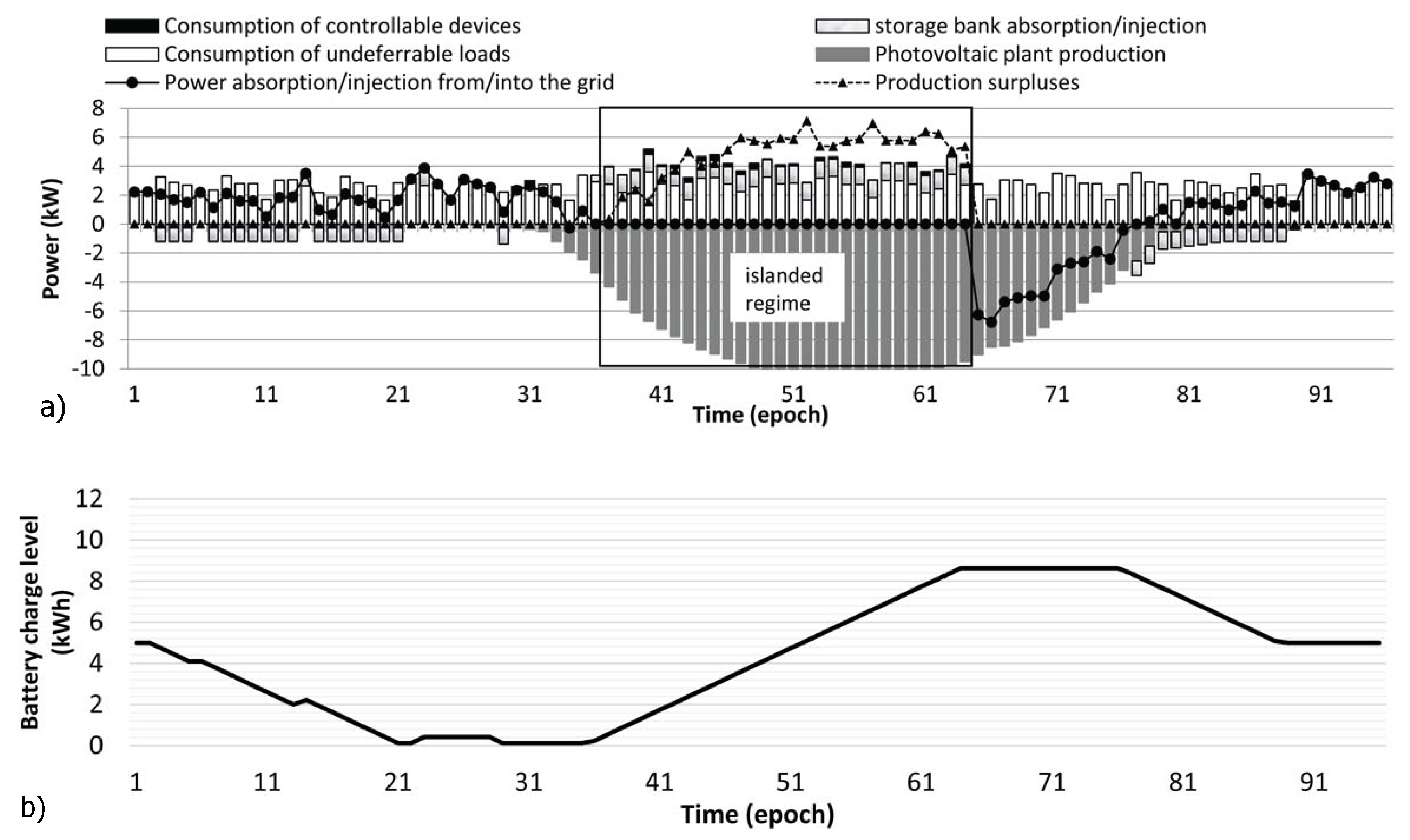
Figure 6 shows the schedules obtained for the same day, assuming that the DSO notifies about an emergency period from Epoch 33 to 64 (i.e., from 8:00 to 16:00). Due to the consistent photovoltaic generation, the EMS manages to avoid energy exchanges with the power grid by operating in islanded mode for most of the emergency time. Note that, when running the smart office in islanded mode, it may happen that the expected PV power production cannot be fully reached due to the power-limited strategy necessary to maintain the power balance and described in Section 3.3. The triangular markers in Figure 6 show the gap between the expected power production of the photovoltaic array operating an MPPT strategy and the actual power production of the photovoltaic panel operating a power-limited strategy.

Conversely, during the cloudy weekday, the photovoltaic production is never sufficient to completely fulfill the energy demand of the smart office. As depicted in Figure 7, in this scenario, there is no convenience in selling energy back to the grid: all of the photovoltaic production is either immediately self-consumed or stored in the battery. However, in this case, the battery charge/discharge cycles are mainly driven by the energy price fluctuations, rather than on the amount of photovoltaic generation. In such a scenario, no request issued by the DSO about islanded operation could be fulfilled.

Figure 5. Energy management system (EMS) schedule of daily energy exchanges with the electricity grid and storage bank charge/discharge periods (a) and storage bank charge level (b). Positive (negative) values indicate energy purchases (sells), energy consumption (production) and battery charges (discharges).

Figure 5. Energy management system (EMS) schedule of daily energy exchanges with the electricity grid and storage bank charge/discharge periods (a) and storage bank charge level (b). Positive (negative) values indicate energy purchases (sells), energy consumption (production) and battery charges (discharges).

Figure 6. EMS schedule of daily energy exchanges with the electricity grid and storage bank charge/discharge periods (a) and storage bank charge level (b) during a sunny weekend day, when maximizing the period of islanded operational mode. Positive (negative) values indicate energy purchases (sells), energy consumption (production) and battery charges (discharges).

Figure 6. EMS schedule of daily energy exchanges with the electricity grid and storage bank charge/discharge periods (a) and storage bank charge level (b) during a sunny weekend day, when maximizing the period of islanded operational mode. Positive (negative) values indicate energy purchases (sells), energy consumption (production) and battery charges (discharges).

Figure 7. EMS schedule of daily energy exchanges with the electricity grid and storage bank charge/discharge periods (a) and storage bank charge level (b) during a partially-cloudy working day. Positive (negative) values indicate energy purchases (sells), energy consumption (production) and battery charges (discharges).

Figure 7. EMS schedule of daily energy exchanges with the electricity grid and storage bank charge/discharge periods (a) and storage bank charge level (b) during a partially-cloudy working day. Positive (negative) values indicate energy purchases (sells), energy consumption (production) and battery charges (discharges).

5. Conclusions

This paper describes an energy management system for a smart office environment, which combines forecasting algorithms for the predictions of energy production/consumption trends with an optimizer that schedules the smart building operations according to the forecasted and actual energy utilization patterns, as well as to the current energy prices. Based on the presented results, we believe that the integration of our proposed system is a valid support to achieve nearly-optimal schedules of the smart building operational mode and to ensure significant cost savings.