1. Introduction
State-of-charge (SoC) estimation is an important issue in the lithium-ion battery area. Without such an estimation system, it is very difficult to avoid the unpredicted-system-interruptions for EVs, and the cells in a pack are easily over-charged and over-discharged [
1,
2,
3]. This will result in permanent damage to the internal structure of the cells. Several methods have been used to estimate the SoC in electrical chemistry laboratories and their accuracy has been verified [
4,
5,
6]. However, estimating the SoC of commercial batteries on-line without destroying them or interrupting the battery power supply is still quite a challenging task for electric vehicle (EV) designers.
The discharge test method is a reliable method to determine the SoC of batteries and the remaining charge can be precisely calculated with it [
7,
8,
9]. However, the time consumed for the testing is very long and after the test, no power is left in the battery, so, it is not appropriate for on-line estimation. The open circuit voltage (OCV) method is another frequently-used method for SoC calibration. Its fundamental principle is that SoC has a special relationship with the embedded quantity of lithium-ion in the active material and there is a one-to-one correspondence between SoC and OCV [
10,
11]. Thus, after adequate resting, the SoC of a battery can be estimated by the open circuit voltage. However, the state-switching (from an operating state to a balanced state) will take up a very long time and its duration is tied to the state of SoC, temperature, and so on, so the OCV method cannot be used for EVs in driving status. To deal with this problem, researchers have developed several model-based SoC estimation methods, in which precise and complex battery models (the combing model, the Rint model, the ESC mode,
etc.) were used for estimating the battery capacity [
12,
13,
14]. With the proposed models, the SoC of batteries can be dynamic estimated on-line. The estimation precisions are largely decided by the models and the collected signals. Many research results demonstrate that the first-order RC model with one-state hysteresis is suitable for LiFePO
4 batteries [
15], but the expensive computational cost makes them unsuitable for EVs with limited calculation resources. In addition, the neural network model method is a nonlinear estimation method, which does not take into account the details of the batteries [
16,
17]. Thus, it is suitable to be used for estimating different kinds of batteries. The drawback of this method is that it needs a great number of training samples and lengthy training procedures.
In practice, many SoC estimation methods have been proposed and most of them estimate the battery state with indirect parameters [
18]. For example, terminal voltage and internal resistance are frequently-used parameters for SoC estimation. However, these parameters always change irregularly when an EV is running in real-life conditiona. Furthermore, the state-of-health (SoH) of a battery has a huge impact on these parameters [
19,
20]. Thus, the SoC estimation methods, relying on these indirect parameters, can hardly obtain precise estimation results.
On the contrary, the Coulomb counting method calculates the remaining capacity by accumulating the amount of the direct parameter—current [
21,
22]. This is a simple and general method, and its precision is defined mainly by the sampling precision and the frequency of the current sensor. Nowadays, many portable devices and electric vehicles, equipped with computable hardware and large memory size, can estimate the remaining battery capacities using this method [
23]. As an open loop SoC estimation method, the errors of the Coulomb counting method are accumulated in the current integral process. As the detection time increases, the cumulative error increases accordingly [
24,
25]. The estimation result is greatly influenced by the precision of the current sensor and the measurement drift, which will result in cumulative effects [
26,
27]. Additionally, the Coulomb counter does not take into account the age and capacity-changes of the battery. Thus, the disadvantages of this method hinder its further application [
28]. For example, the Coulombic efficiency is greatly influenced by the operating status of the battery (SoC, temperature and current) and this is difficult to measure [
29,
30,
31,
32].
To deal with this problem, we propose a lossy counting-based relative Coulomb counting method for estimating the available capacity or SoC of lithium-ion batteries. The initial capacity of the tested battery is obtained with the OCV-SoC curve. The charging/discharging efficiencies, used for compensating the Coulombic losses, are dynamically corrected by a lossy counting method. The measurement drift, coming from the current sensor, is amended with a relative accumulating manner of charge.
The rest of this paper is organized as follows: we first reviewed the related work on the lossy counting method (LC). Secondly, we present the LC-based SoC or available capacity estimation method for lithium-ion batteries. Then we describe several experiments, in which different parameters of the algorithm are examined. With these experiments, we demonstrated how to accumulate the summary information and to calculate the SoC or available capacity for the proposed algorithm. Finally, we concluded this paper by highlighting the key contributions of this work.
3. LC-Based SoC Estimating Method
In fact, under actual driving conditions, it is very hard to accurately calculate the SoC or available capacity with the estimated Coulombic efficiency needed by Equation (1) during the whole charge or discharge process. Many factors have effects on the Coulombic efficiency and the calculation result. Thus, accumulating the measured current and correcting it with an accurate Coulombic efficiency at each measurement point perhaps is the only feasible way. Under such a condition, Equation (1) can be substituted by Equation (3), where
I(
t),
T(
t), SoC(
t), SoH(
t) are the current, temperature, SoC and SoH of the battery at time
t:
In practice, the sensors can only send data at every discrete time point,
tk (tk = Δ
t × k). Δ
t is the sampling interval and
k is the number of sampling. Thus, we can get:
Generally speaking, the definition domain of Coulombic efficiency, η, is continuous. It is impossible to obtain an accurate η for each point in the definition domain. Thus, we have to discretize the definition domain into lattices with the same size. In the same lattice, the Coulombic efficiencies of these points are set to the same values. Thus:
Having discretized the whole definition domain into lattices and calculated the whole capacity for points in the same lattice, we can number these lattices with “
L1,
L2,
…,
Ln” and calculate the SoC of battery with Equation (3),
In fact, accurately determining these Coulombic efficiencies,
, is a hard thing. The relationship between the discharge capacity and the operating current/battery temperature/SoH is complicated and nonlinear. In the
kth cycle, the released capacity
can be expressed like this:
where
= η
× Qk + where η = {
,
,
…,
} be the vector of Coulombic efficiency,
Qk = {
, ,
…,
} be the accumulated capacities for lattices,
be the error.
Having implemented
K cycles, we can obtain the matrix:
There are many methods that can be used to estimate the unknown parameter η as long as
Ln ≤ K. In this paper, we estimate η with the least square method. The minimized sum of squares is:
To solve the extreme-value problem, we can get:
In this way, the Coulombic efficiency, η, can be calculated after
K(Ln =
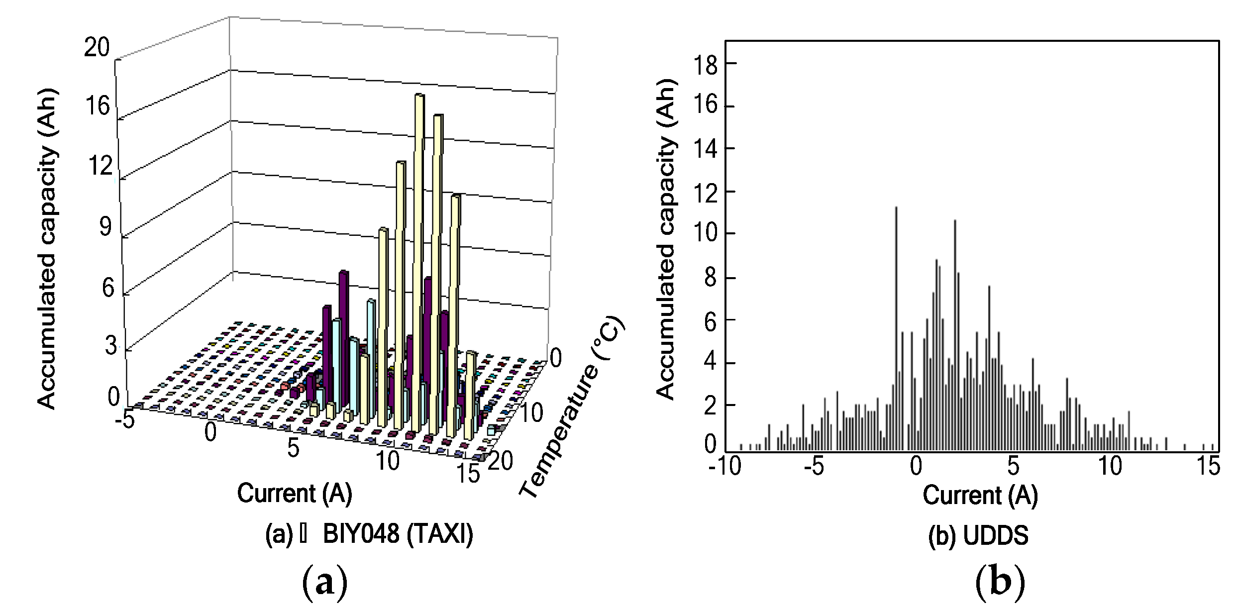
K) time running and it can be refreshed every time a charge/discharge process has been completed. In fact, the accumulated capacities of lattices are quite different. This can be observed in
Figure 3, in which
Figure 3a is the statistical capacity distribution of an EV-taxi in two-dimensional space, and
Figure 3b is the statistical capacity distribution in the Urban Dynamometer Driving Schedule (UDDS) in one-dimensional space.
From both of them, we can see that most of these capacities converged in several special lattices, so discretizing the definition domain into lattices and calculating the SoC with the revised η for each accumulated capacity is a suitable way to estimate the SoC or available capacities for batteries.
Figure 3.
The capacity distributions in different driving cycles. (a) Jing BIY048 (TAXI); (b) UDDS.
Figure 3.
The capacity distributions in different driving cycles. (a) Jing BIY048 (TAXI); (b) UDDS.
3.1. The LC-Based Relative Coulomb Counting Method
Definition 5. (Bucket, bj). Let the measured values of current, temperature, SoC and SoH, I(tk), T(tk), SoC(tk), and SoH(tk), be a data stream, the incoming stream is conceptually divided into buckets. Each bucket has ΔQ × (1/ϵ) Ah capacity and is labeled by bj = Qk/(ΔQ × (1/ϵ)). (Qk is the total accumulated capacity from time t0 to tk and ΔQ is unit capacity)
Definition 6. (Data structure, DS). DS is a set of entries, in the form (I*(tk), T* (tk), SoC* (tk), SoH* (tk), Q, Δ), where I* (tk), T* (tk), SoC* (tk), SoH* (tk) are the discretized values for I(tk), T(tk), SoC(tk), SoH(tk). Q is the accumulated capacity for entry (I*(tk), T* (tk), SoC* (tk), SoH* (tk)). Parameter tk is the measurement time at the kth time-step. Δ is the maximum possible error in Q.
| Algorithm |
(1): Initializing DS. Clear the records in it. Initialize the error ϵ, support s and unit capacity ΔQ. (2): Recording data. For every time interval tk, read in the measured values for I(tk), T(tk), SoC(tk), SoH(tk) and discretize these measured values, I*(tk) = INT(I(tk)), T* (tk) = INT(T(tk)), SoC* (tk), = INT(10 × SoC(tk))/10, SoH* (tk), = INT(10 × SoH(tk))/10. Having done this, calculate the discharge/charge capacity for the discretized lattice, Q (tk) = I(tk) × (tk − tk–1). (3): Look up DS to see whether or not an entry, (I*(tk), T*(tk), SoC* (tk), SoH* (tk), Q, Δ), has existed. If there is any, update the entry by increasing the capacity for it (Q = Q + Q(tk)). Otherwise, establish a new entry (I*(tk), T* (tk), SoC* (tk), SoH* (tk), Q = Q(tk), Δ = ΔQ × (bj –1)) for it. (4): Does a bucket boundary arrive? Yes, go (5); No, go (2). (5): Prune DS by deleting the entries in it and go (2). The rule for deletion is “for an entry (I*(tk), T* (tk), SoC* (tk), SoH* (tk), Q,Δ), if Q + Δ ≤ ΔQ × bj, then delete it”.
|
Whenever a user asks for the capacity list of items with threshold
s, the entries (
Q ≥ (
s − ϵ) × Δ
Q ×
k) will be outputted. Thus, with the obtained list (the entries (
Q <
(s − ϵ
) × Δ
Q ×
k) were seen as zero), the SoC can be calculated by:
3.2. Algorithm Analysis
Theorem 1: Let ((I*(tk), T* (tk), SoC* (tk), SoH* (tk)), Q,Δ) be an entry in the data structure DS, I* (tk), T* (tk), SoC* (tk), SoH* (tk) are the discretized values for I(tk), T(tk), SoC(tk), SoH(tk) at time tk, Q be the accumulated capacities of (I*(tk), T* (tk), SoC* (tk), SoH* (tk)), Δ be the maximum possible capacity error in Q, bj be the label of a bucket, k be the discrete time-step, ϵ be the given error, s be the given support degree, ΔQ be the given unit capacity. Let QI*(tk), T* (tk), SoC* (tk), SoH* (tk) be the true capacity for (I*(tk), T* (tk), SoC* (tk), SoH* (tk)).
Then,- (A)
If ((I*(tk), T* (tk), SoC* (tk), SoH* (tk)), Q, Δ) does not appear in DS, then QI*(tk), T* (tk), SoC* (tk), SoH* (tk) ≤ Qk × ϵ;
- (B)
If ((I*(tk), T* (tk), SoC* (tk), SoH* (tk)), Q, Δ) appears in DS, then Q ≤ QI*(tk), T* (tk), SoC* (tk), SoH* (tk) ≤ Q + Qk × ϵ;
- (C)
If (for every time interval tk, Q(tk) > ΔQ) is true, then, with the given error ϵ, the algorithm computes the distribution synopsis using at most entries.
Proof: According to definition 5, we can get bj = Qk/(ΔQ × (1/ϵ)).
For the first bucket (bj = 1), an entry ((I*(tk), T* (tk), SoC* (tk), SoH* (tk)), Q, Δ) is deleted only when the capacity of it, Q ≤ ΔQ × bj. Q is also the true capacity of (I*(tk), T* (tk), SoC* (tk), SoH* (tk)). Thus, QI*(tk), T* (tk), SoC* (tk), SoH* (tk) ≤ ΔQ × bj = Qk × ϵ.
For an entry ((I*(tk), T* (tk), SoC* (tk), SoH* (tk)), Q, Δ) that gets deleted in the other buckets (bj > 1), which was inserted into the DS when bucket bj = Δ/ΔQ + 1 was being processed, the capacity Q of it is the additional capacity after the insertion. Thus, the true capacity of (I*(tk), T* (tk), SoC* (tk), SoH* (tk) in bucket bj was no more than Q + Δ. According to the deletion rule appeared in step (5), we can get Q + Δ ≤ ΔQ × bcurrent = Qk × ϵ. Thus, conclusion (A) is true.
In the first bucket (bj = 1), if the capacity of an entry Δ = 0, then Q = Q I*(tk), T* (tk), SoC* (tk), SoH* (tk). In other buckets, entry ((I*(tk), T* (tk), SoC* (tk), SoH* (tk)), Q, Δ) is deleted at most Δ/ΔQ times. If an entry appeared in the current bucket bcurrent, the true capacity of it QI*(tk), T* (tk), SoC* (tk), SoH* (tk) will no more than Q + Δ. Since Δ ≤ ΔQ × (bcurrent − 1) ≤ Qk × ϵ, we can get Q ≤ QI*(tk), T* (tk), SoC* (tk), SoH* (tk) ≤ Q + Qk × ϵ. Thus, conclusion (B) is true.
Let
bcurrent be the current bucket id,
j ϵ [1,
bcurrent],
ej be the number of entries in data structure DS, whose bucket id is (
bcurrent –
bj + 1). Then, the accumulated capacities of these entries appeared in such a bucket (
bcurrent − bj + 1) must be greater than Δ
Q ×
bj. Otherwise, it would have been removed. Let the size of the buckets is Δ
Q × (1/ϵ), thus, we can get:
When
h = 1, the inequality Equation (11) can be changed into
. After transformation, we can get:
In this way, when
h = 1, 2, …,
bcurrent, we can get:
Since |
bcurrent| =
, we can get:
Thus, conclusion (C) is true.
From conclusions (A)–(C), we can find that when the entries tend to uniformly distribute at random, the proposed algorithm can obtain the summary information of the accumulated current with very low space. At the same time, the statistical accuracy is guaranteed.
4. Experiments
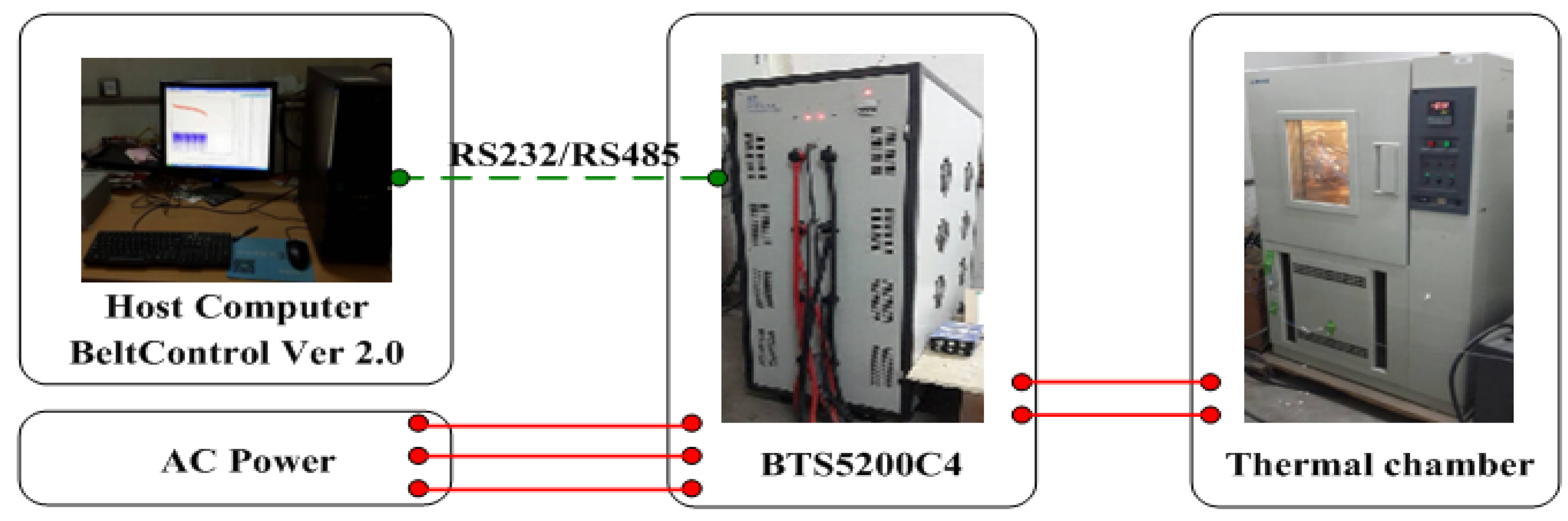
The test bench, which consists of a thermal chamber for environment control, a host computer, a BaTe battery test system NBT BTS5200C4 and BeltControl 2.0 interface for programming the NBT BTS5200C4 is shown in
Figure 4. The maximum voltage, maximum charge/discharge current, current control accuracy and voltage control accuracy of the NBT BTS5200C4 were 5.0 V, 200A, ± (0.1%FD + 0.1%RD) and ± (0.1%FD + 0.1%RD). In fact, the device can record the experimental data including temperature, current, voltage, accumulative amp-hours (Ah) and watt-hours (Wh). The host computer can collect the data through RS232/RS485 protocol. Four LFP cells (Battery-1, Battery-2, Battery-3 and Battery-4) were utilized to examine the accuracy of the proposed algorithm.
Figure 4.
The battery test bench.
Figure 4.
The battery test bench.
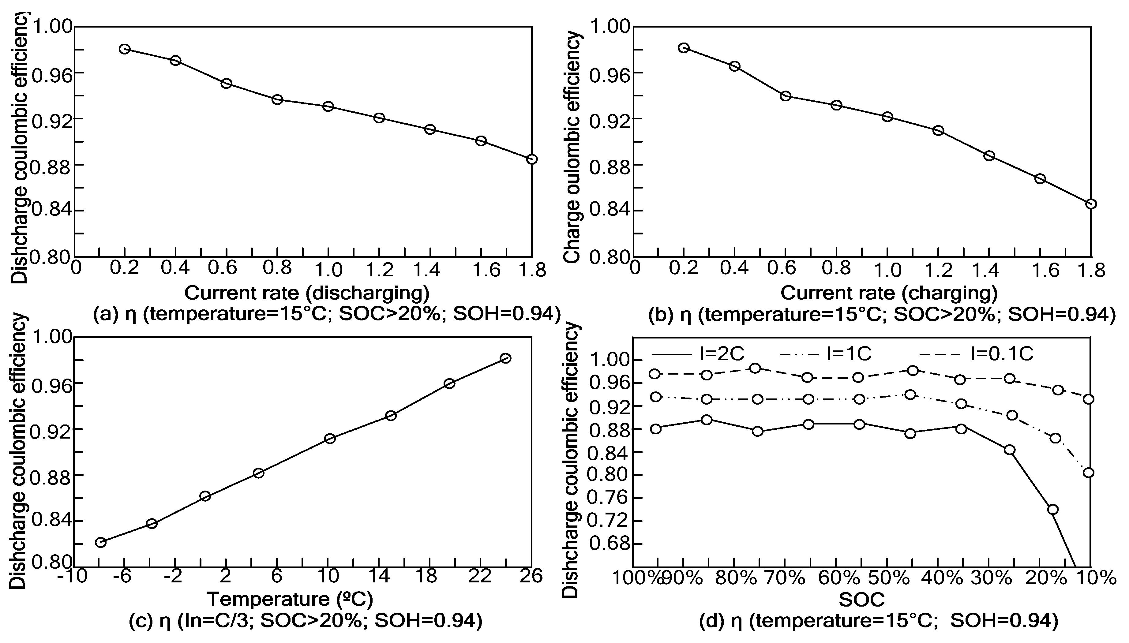
4.1. How to Reduce the Dimension of Coulombic Efficiency, η
Generally speaking, the Coulombic efficiency η is a function of current, temperature, SoC and SoH. From Equations (3) and (4) we can see that, to obtain an accurate value of SoC or available capacity, we have to discretize the definition domain of η into more lattices. This will lead to more expense. In fact, for an EV or HEV, the Coulombic efficiencies of the batteries are greatly affected by the fluctuations of discharge current and environmental temperature, slightly or slowly affected by SoC and SoH. In a short-term running, the change of SoH is very little. In the SoC range of 20%–100%, the Coulombic efficiency at the same temperature, SoH and charge/discharge current remains almost unchanged. This can be observed in
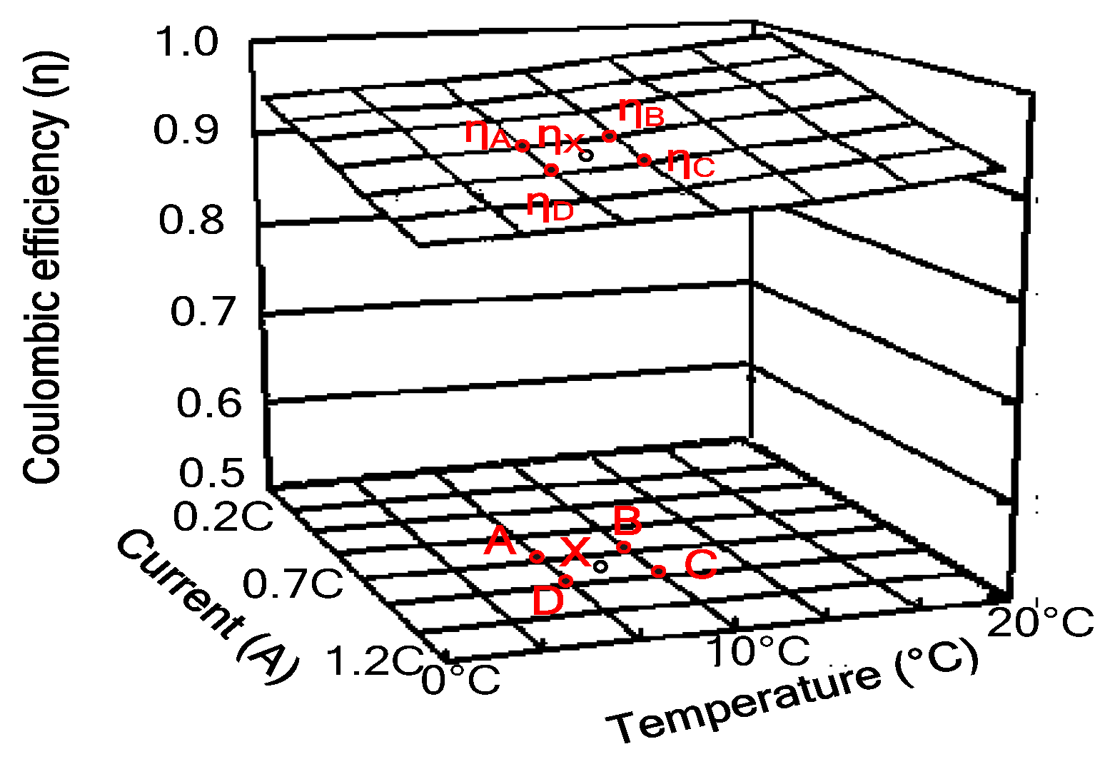
Figure 2d. Thus, we can discretize the definition domain of η only in two-dimension space and initialize only several key Coulombic efficiencies in this space. The Coulombic efficiencies of other points can be calculated by the four key points nearby. This can be seen from
Figure 5, in which the Coulombic efficiency of point X is calculated by comparing with the Coulombic efficiencies of four other key nearby points. With the given function,
zp =
a0 +
a1xp +
a2yp +
a3xpyp and four nearest key points, A, B, C and D, the Coulombic efficiency of point
X, η
X, can be easily calculated by solving the equation.
Figure 5.
The Coulombic efficiencies of critical and non-critical points.
Figure 5.
The Coulombic efficiencies of critical and non-critical points.
4.2. The Influences of Discharge Order and Frequency
From Equation (7) we can see that the proposed LC-based available capacity estimation method can calculate the accumulated capacities for lattices. However, the discharging order and frequency of these lattices cannot be recorded in the accumulation process. The discharging order and frequency are some other parameters which possibly influence the calculated available capacity. To make this point clear, several experiments were conducted and the results are shown below.
4.2.1. The Influences of Discharge Order
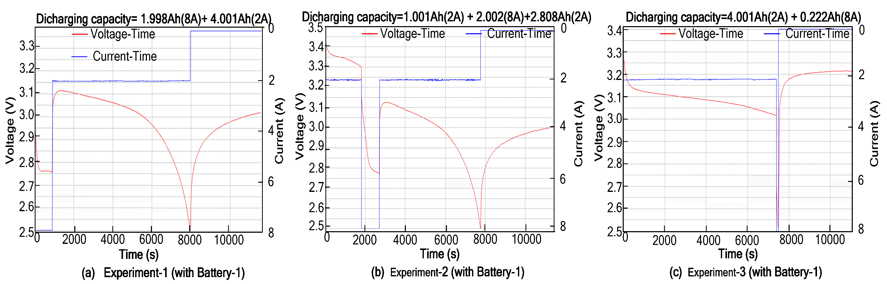
To examine the influence of discharge order on the obtained available capacity, three experiments were conducted on Battery-1. In Experiment-1, a total of two discharge procedures were carried out. The battery was firstly required to discharge at 8 A for 2 Ah and then discharged at 2 A until the voltage reaches the discharge threshold. This can be observed in
Figure 6a, where the discharged capacity of battery-1 at 2 A is 4.001 Ah. In Experiment-2, the battery was firstly required to discharge at 2 A for 1 Ah, and then, discharge at 8 A for 2 Ah. Finally, it is discharged at 2 A until the voltage reaches the discharge threshold (2.5 V). This can be observed in
Figure 6b. In Experiment-3, the battery was firstly required to discharge at 2 A for 4.001 Ah and then, discharged at 8 A for 0.222 Ah. After each of these experiments, the battery was required to rest for 1 h.
By comparing the three discharge experiments, we can find that without calculating the Coulombic efficiency, the total discharge capacities of the three experiments are not equal. The capacity difference between Experiment-1 and Experiment-2 is very small (1.998 + 4.001 − 1.001 − 2.002 − 2.808 = 0.188 Ah). The capacity difference between Experiment-1 and Experiment-3 is “1.998 + 4.001 − 4.001 − 0.222 = 1.776 Ah”. This is very large for a low-capacity battery.
In fact, discharge order has no noticeable influence on the discharge capacity. The reason (why the discharged capacities, in Experiment-1 and Experiment-3, were so different?) lies in the insufficient power of the battery in Experiment-3. In
Figure 6c, having discharged most of its capacity (4.001 Ah + 0.222 Ah), Battery-1 does not have sufficient power to maintain the discharging process. Thus, with the large discharge impedance, the voltage quickly falls to the cut off voltage (2.5 V). It is a fake fully-discharged-state and the SoC in Experiment-3 didn’t reach zero. We can verify this by adding a resting stage (1 h) after each discharging experiment. Having done so, we found that the difference between the two open circuit voltages in Experiment-1 and Experiment-2, was very unimportant (3.10 − 3.06 = 0.04 V). In Experiment-1 and Experiment-3, the difference was very considerable (3.10 − 3.23 = −0.13 V). For a lithium-ion battery, the OCV-SoC charging or discharging curve is a flat one. A little difference in terminal voltage will lead to a huge gap in SoC. Thus, we can say that Battery-1 reaches similar states in Experiment-1 and Experiment-2. In Experiment-3, the its terminal status was distinct from the other cases, so it cannot be used to examine the influence of discharge order for the scheduled discharging procedure (8 A/2 Ah) was not completed.
From the experiments above, we can get the conclusion that, as long as the discharging power and cut off voltage were rightly controlled, discharge order has no obvious influence on discharge capacity.
Figure 6.
The influences of discharge order. (a) Experiment-1 (with Battery-1); (b) Experiment-2 (with Battery-1); (c) Experiment-3 (with Battery-1).
Figure 6.
The influences of discharge order. (a) Experiment-1 (with Battery-1); (b) Experiment-2 (with Battery-1); (c) Experiment-3 (with Battery-1).
4.2.2. The Influences of Discharge Frequency
From Equations (3)–(7) and
Figure 3, we can see that the accumulated capacities of the lattices can be achieved by the proposed LC-based SoC estimation method, but the frequencies of different charge/discharge operations cannot be recorded by the proposed algorithm.
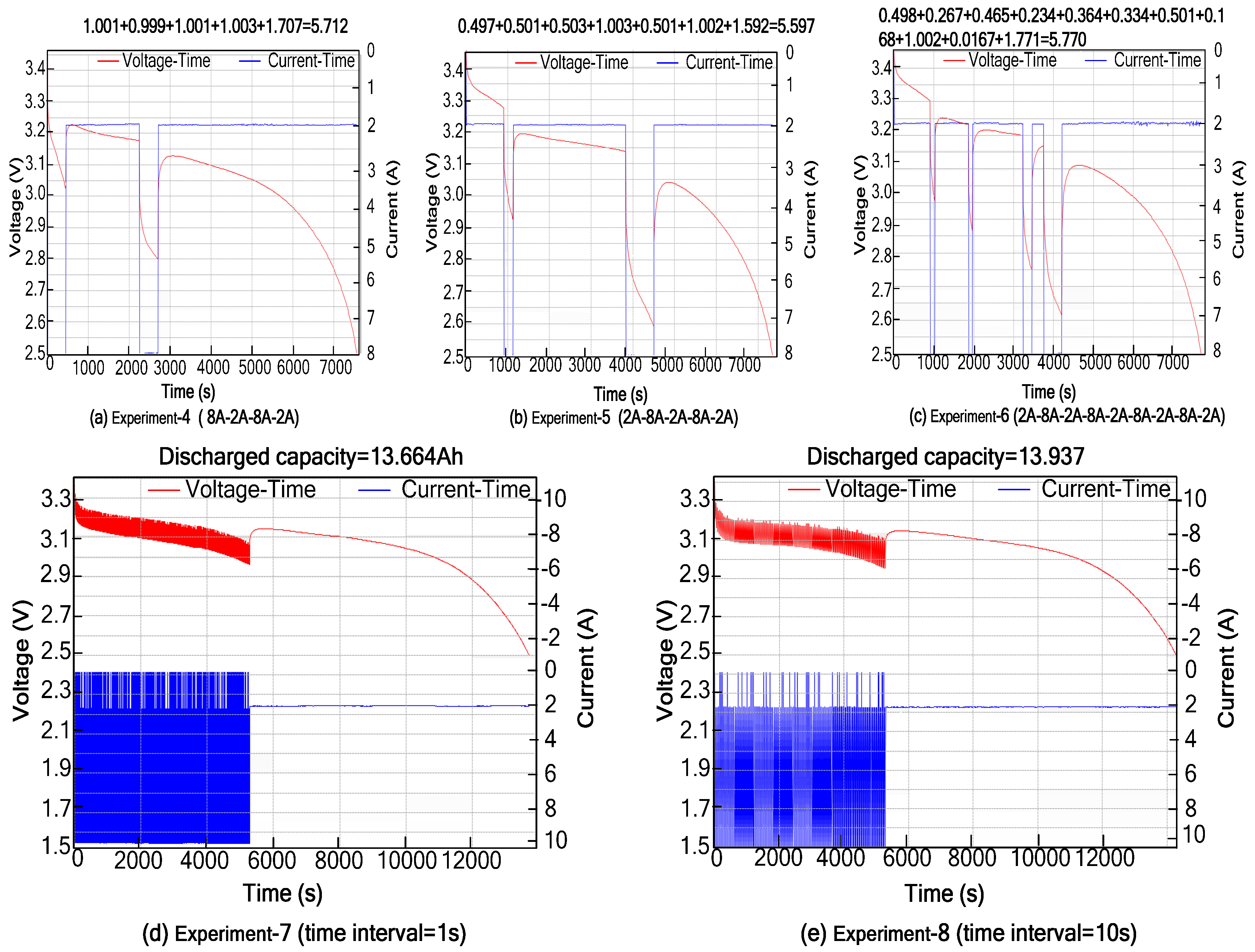
To examine the low-frequency feature of the proposed algorithm, three discharge experiments were performed on Battery-2. All of these experiments include two kinds of discharge steps. In step-1, the discharge current is 8 A. In step-2, the discharge current is 2 A. In all of these experiments, both the discharge capacities in step-1/step-2 are 2 Ah. Having consumed the scheduled capacity for step-1 (2 Ah) and step-2 (2 Ah), discharge procedures keep discharging at a 2 A rate until the voltage threshold is reached. From
Figure 7a–c, we can see that the total discharge capacities of the three experiments are 5.712 Ah, 5.597 Ah and 5.770 Ah. The differences between them are very small.
Figure 7.
The discharge procedures with different discharging frequencies. (a) Experiment-4 (8A-2A-8A-2A); (b) Experiment-5 (2A-8A-2A-8A-2A); (c) Experiment-6 (2A-8A-2A-8A-2A-8A-2A-8A-2A); (d) Experiment-7 (time intervals = 1 s); (e) Experiment-8 (time intervals = 10 s).
Figure 7.
The discharge procedures with different discharging frequencies. (a) Experiment-4 (8A-2A-8A-2A); (b) Experiment-5 (2A-8A-2A-8A-2A); (c) Experiment-6 (2A-8A-2A-8A-2A-8A-2A-8A-2A); (d) Experiment-7 (time intervals = 1 s); (e) Experiment-8 (time intervals = 10 s).
To examine the high-frequency features of the proposed algorithm, we further implemented two high-frequency discharge experiments on Battery-3. Their discharge intervals are 1 s and 10 s. The scheduled capacities
(C1 and
C2
) for discharge current-1 (10 A) and current-2 (2 A) in the two experiments are the same. Having consumed the accumulated capacities,
C1 and
C2, discharge procedures keep discharging at a 2 A rate until the discharge voltage threshold is reached. From
Figure 7d–e, we can also find that the total discharge capacities of the two experiments are very similar. One is 13.664 Ah, the other is 13.937 Ah. Thus, we can say that the discharge capacity has no relation to discharge frequency.
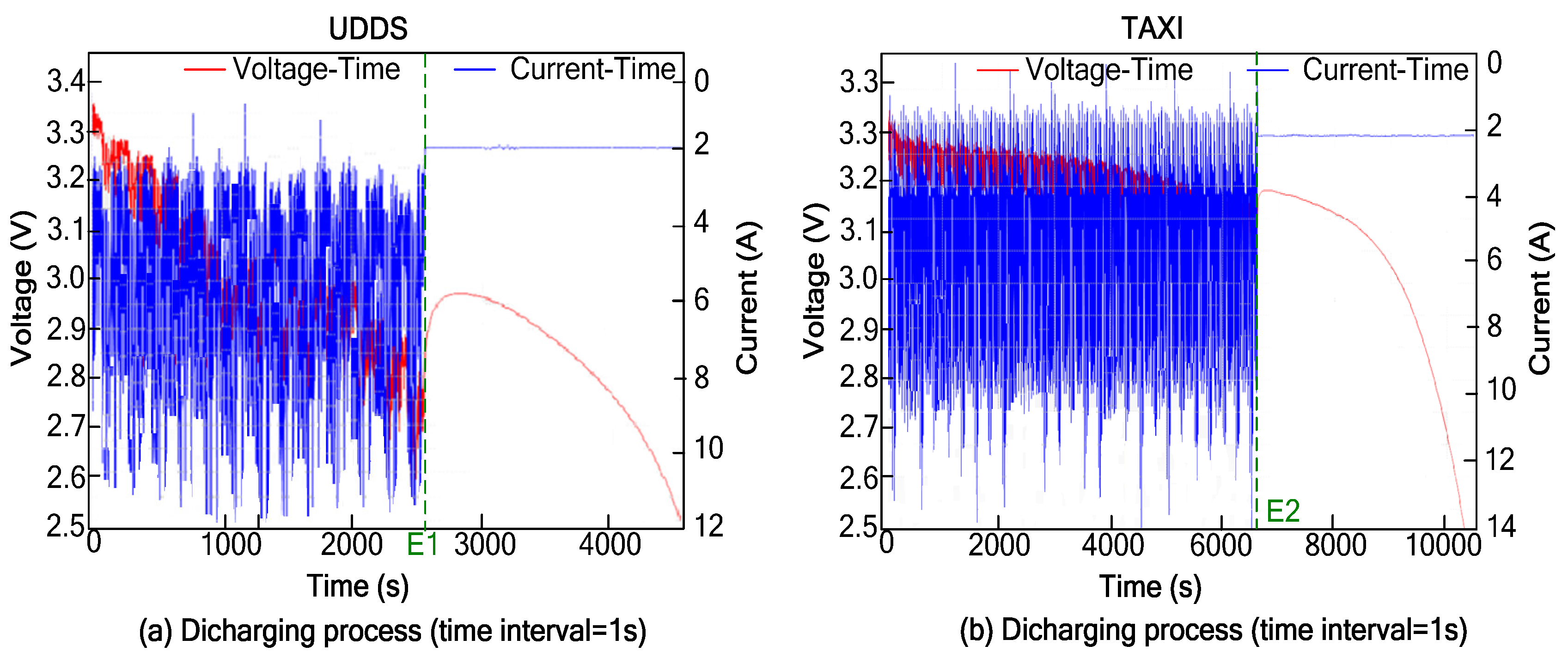
4.3. Verification of the Proposed Estimation Method
Figure 8 illustrates the process of the verification experiment for the proposed LC-based estimation method. Two kinds of discharging cycles (UDDS and TAXI) were used for testing the proposed algorithm. Both experiments were performed at 10 °C. The current, voltage and operating time were examined every 0.1 s, 1 s, 2 s, 5 s, 10 s and 20 s. Before the examination point (
E1
/E2), the discharging process was conducted with the given driving cycles. After them, the battery was discharged with 2 A to the cut-off voltage. The discharge current is discretized into 10 lattices, and 10 Coulombic efficiency coefficients were initialized to 1. In fact, the charge/discharge capacity, obtained at different currents, can be transformed into an equivalent capacity at a constant current. In this section, the constant current is set to 2 A and the discharge Coulombic efficiency of 2 A, η
2A, is artificially set to 1. Thus, the equivalent discharged capacity (
Q`j) for variable current
j can be expressed by
Q`j = η
j·
Qj/η
2A, where
Qj is the accumulated capacity for current
j, η
j is the Coulombic efficiency for current
j. Thus, the estimated equivalent discharged capacity at the examined point
E1,
Qi,(0~E1), can be calculated by:
After 10 discharging cycles, we obtained the equation set below:
In both experiments, the available capacity
CN was defined as the discharged capacity of the battery at the discharging current 2 A. Thus, for each of the discharge cycle
i, the true equivalent discharged capacity of it at the examination point
E1,
Qi,(0~E1)*, can be expressed by
Qi,(0~E1)* =
CN −
Qi,(E1~END). Qi,(E1~END) is the discharge capacity of the battery at 2 A, from time
E1 to the end. In this way, equation set Equation (14) can be modified into Equation (15):
Thus, if we initialize the Coulombic efficiency, η = {, , …, }, with 1 in the first 10 equations, and accumulate the capacities for lattices in each discharge cycle. After running ten times, the accurate Coulombic efficiencies will be obtained with Equations (9) and (10), gradually.
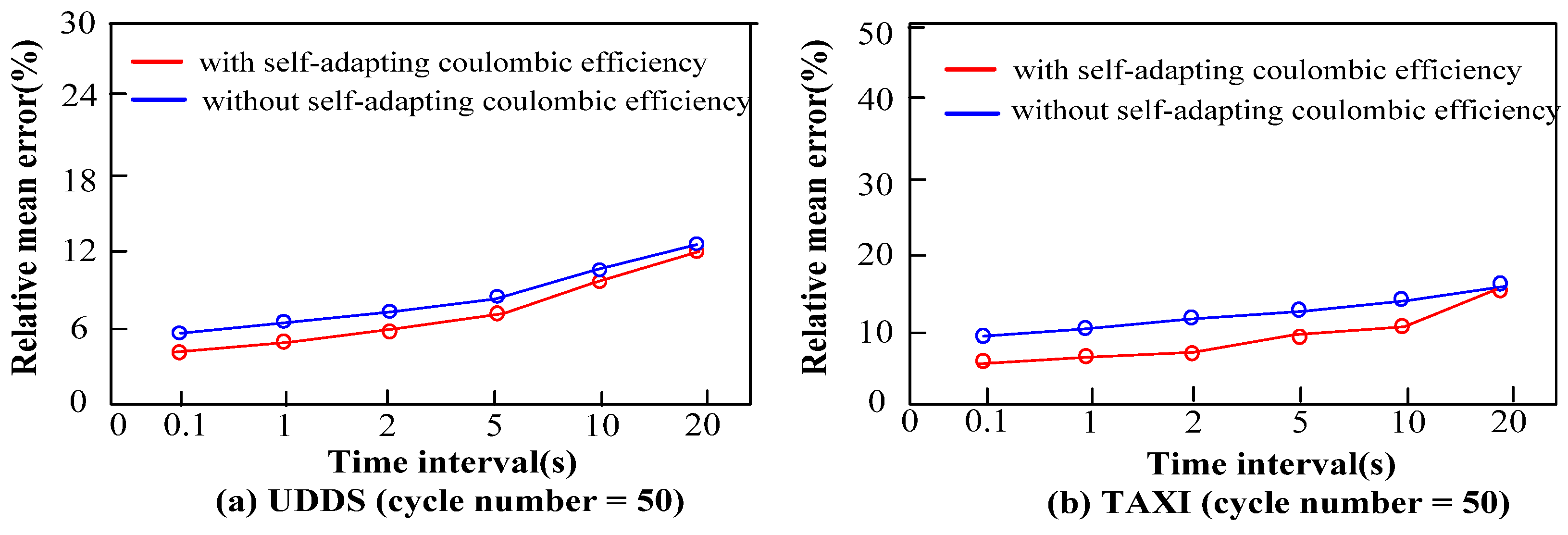
In
Figure 9, two kinds of Coulomb counting methods are shown. Charge/discharge cycles were carried out fifty times. We analyzed the performance of the two algorithms by comparing their relative mean errors. The red line indicates the relative mean errors between the real residual capacity and the estimated residual capacity. Real residual capacity is obtained by discharging the battery with 2 A, from the examination point to the cut-off voltage. The estimated residual capacity is achieved with the proposed algorithm. The blue line is the relative mean error obtained with the traditional Coulomb counting method. It can be observed in
Figure 10a,b that, on the one hand, with the increase of the time interval, the relative mean error gets larger and larger. On the other hand, the changing rates of the errors in the two algorithms are different. With the increasing time interval, the relative mean errors of the two algorithms get more and more similar.
Figure 8.
Two different discharging procedures (a) UDDS; (b) TAXI.
Figure 8.
Two different discharging procedures (a) UDDS; (b) TAXI.
Figure 9.
Relative mean errors of two different Coulomb counting methods. (a) UDDS; (b) TAXI.
Figure 9.
Relative mean errors of two different Coulomb counting methods. (a) UDDS; (b) TAXI.
4.4. The Influences of Measurement Interval
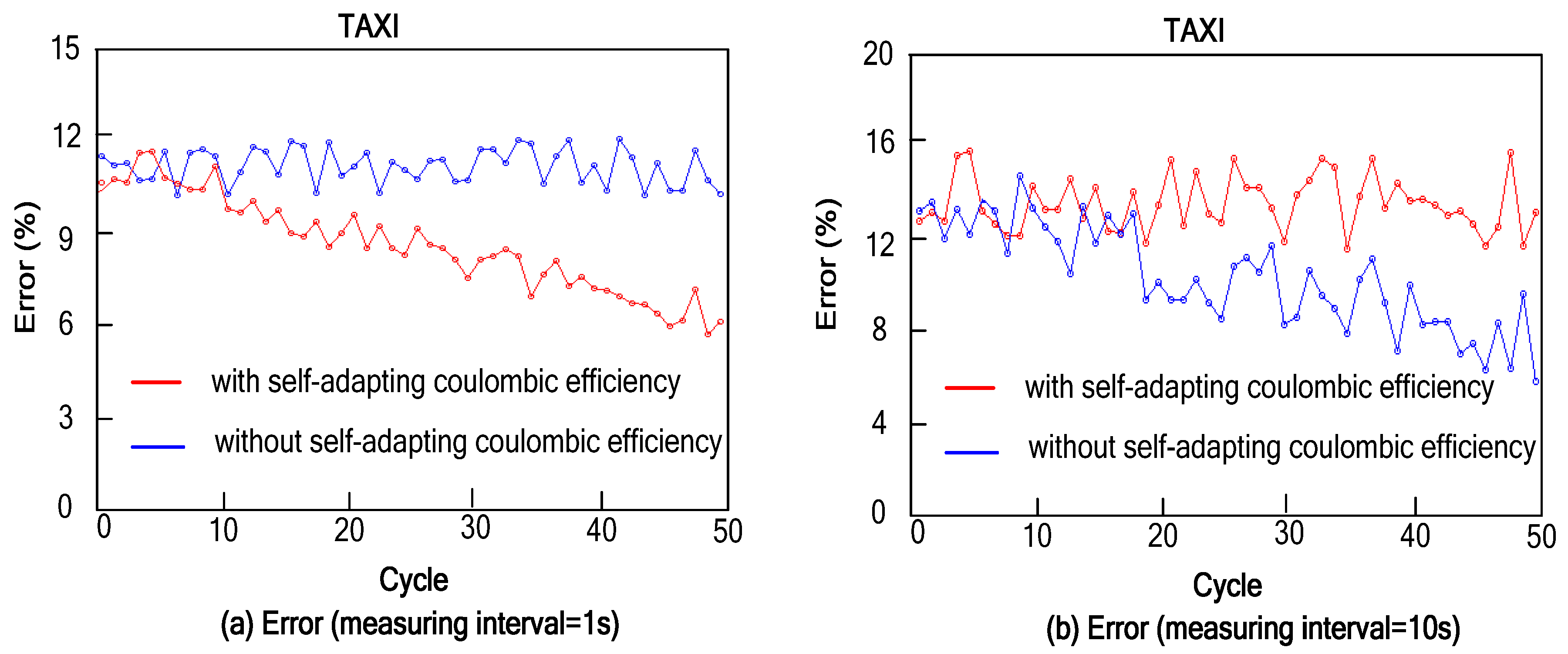
To further illustrate the impact of measurement time interval, we compared the estimation errors when the interval was set to 0.1 s, 1 s and 10 s. An actual discharging cycle, TAXI, was used to measure the errors. The experiment was carried out at 10 °C and the discharge current was discretized into 10 lattices. With the proposed method and the traditional method, we obtained the errors when the measurement interval was set to different values.
It can be observed in
Figure 10a,b that, in the former ten driving cycles, the errors obtained with the two algorithms remain similar. However, after 10 implementations, the obtained results with the two algorithms are quite different. For the traditional Coulomb counting method, since no correction is carried out on the Coulombic efficiency, its estimation errors remain almost unchanged. For the proposed algorithm, by introducing the self-adapting Coulombic efficiency coefficient, η, the estimation error is reduced to nearly 5% and 6%, step by step. In the two methods, both the average error and the variation range of errors were enlarged when the measurement time interval was changed from 1 s to 10 s. It is quite conceivable that a larger measurement interval leads to a larger accumulated error, but accurate measurement means high computational cost and expensive devices.
In
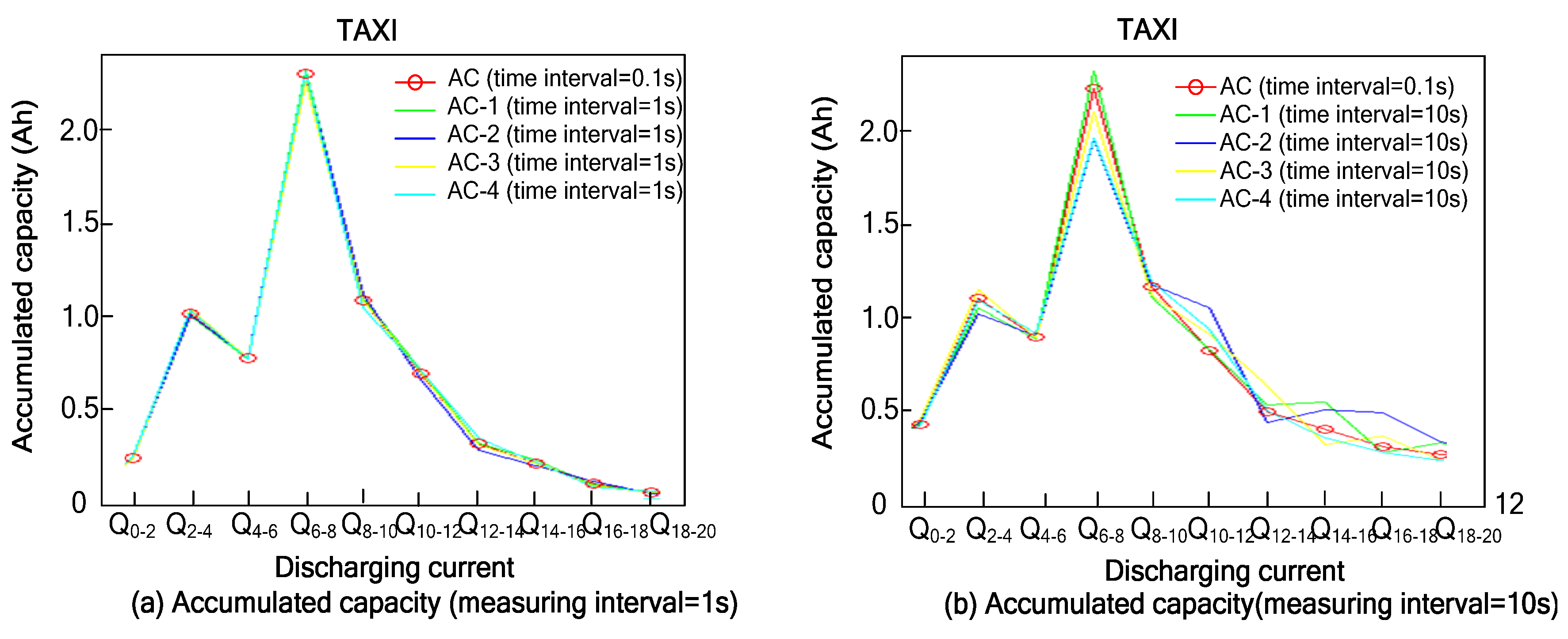
Figure 11, the accumulated capacities of ten current-intervals are shown. In
Figure 11a, four different measuring procedures were performed. In both, the measurement intervals were set to 1s. In
Figure 11b, four measurement intervals were set to 10 s. For both figures, the accumulated capacity, AC (measurement interval = 0.1 s), was seen as a basis of reference. Thus, with the comparison we can find that the capacity difference between the measurement intervals of 0.1 s and 1 s is very little. This will lead to less error. On the contrary, the accumulated capacity difference between 0.1 s and 10 s is very large. Thus, it cannot be used to estimate the Coulombic efficiency coefficient, η, for an EV. In fact, “measurement interval = 0.1 s” is enough for an EV. Below it, no further benefit will be achieved and the profit coming from improving the measurement interval will be eroded by noise.
Figure 10.
Estimation errors of two different Coulomb counting methods. (a) Measuring interval = 1 s; (b) Measuring interval = 10 s.
Figure 10.
Estimation errors of two different Coulomb counting methods. (a) Measuring interval = 1 s; (b) Measuring interval = 10 s.
Figure 11.
Accumulated capacities for different discharging currents. (a) Measuring interval = 1 s; (b) Measuring interval = 10 s.
Figure 11.
Accumulated capacities for different discharging currents. (a) Measuring interval = 1 s; (b) Measuring interval = 10 s.
4.5. The Influences of Noise
To further discuss the influence of the sensor noise, two kinds of noise were overlaid on the original current signals. The accumulated capacities for different lattices in the discharging cycle are shown in
Figure 12, from which we can see that, when noise (−0.1 A–0.1 A) was overlaid on the original current signals, the distribution and total quantity of the accumulated charge obtained on the synthetic signals (red lines) were very similar to those in the original current signals (blue lines). When noise (0 A–0.2 A) was overlaid on the original signals, the distribution and the total accumulated charge on the synthetic signals (green lines) differed from those in the original signals (blue lines).
Figure 12.
The accumulated capacities in different noisy environments.
Figure 12.
The accumulated capacities in different noisy environments.
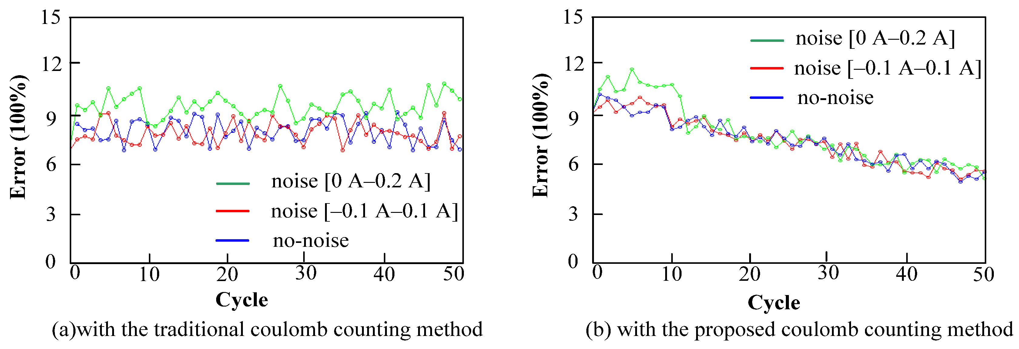
Though the obtained current information was overlaid with the same noise signal, the relative errors obtained by the traditional Coulomb counting method and the proposed Coulomb counting method were quite different. This can be observed in
Figure 13a,b, where three variation trends of the relative errors in different noise conditions were shown, respectively. By comparing
Figure 13a and
Figure 13b we can find that when noise (−0.1 A–0.1 A) was overlaid on the original current signals, the ranges (or trends) of the relative errors obtained with the two Coulomb counting methods remained unchanged. However, when noise (0 A–0.2 A) was overlaid on the original current signals, the relative errors obtained with the traditional Coulomb counting method increased, but the trend (or range) of the relative error obtained with the proposed Coulomb counting methods remained unchanged (in the latter 40 discharging cycles).
The answer resides in the equation set of Equation (15). When noise (0 A–0.2 A) was overlaid on the original current signals, all of the accumulated capacities for lattices Ln, QLn,i were increased. In the former 10 residual capacity calculation, the Coulombic efficiency, for each lattice cannot be revised, so the obtained errors will increase. However, after running 10 times (10 equations), the Coulombic efficiency , begins to be revised dynamically. Although the Coulombic efficiencies, , were changed into distorted values as the polluted capacities, QLn,i, were introduced, the ultimate estimation error is very small as the interaction effects exists.
Figure 13.
The relative errors in different noisy environments. (a) With the traditional coulomb counting method; (b) With the proposed coulomb counting method.
Figure 13.
The relative errors in different noisy environments. (a) With the traditional coulomb counting method; (b) With the proposed coulomb counting method.
The changing specific process can be seen in
Figure 14, where the values of two Coulombic efficiency, η
[4A-6A] and η
[8A-10A], were shown in
Figure 14a,b. The corresponding accumulated capacities, Q
[4A-6A] and Q
[8A-10A] were presented in
Figure 14c,d. With the intervention of the noise, the accumulated capacities, Q
[4A-6A] and Q
[8A-10A], increased in the total 50 driving cycles. However, the corresponding Coulombic efficiencies, η
[4A-6A] and η
[8A-10A], remain unchanged in the former 10 runs and decreased in the latter 40. Since no revision was carried out in the former 10 driving cycles (the values of η
[4A-6A] and η
[8A-10A] kept unchanged), the relative errors obtained in the former 10 driving cycles were larger than that in the latter 40 driving cycles. Additionally, with the increasing noise (from [0 A–0.1 A] to [0.1 A–0.2 A]), the accumulated capacity was enlarged. The reverse movement of the Coulombic efficiency makes the final error decrease.
Figure 14.
The relative errors in different noisy environments. (a) η[8A-10A]; (b) η[4A-6A]; (c) Q[8A-10A]; (d) Q[4A-6A].
Figure 14.
The relative errors in different noisy environments. (a) η[8A-10A]; (b) η[4A-6A]; (c) Q[8A-10A]; (d) Q[4A-6A].


