Optimal Real-Time Scheduling of Wind Integrated Power System Presented with Storage and Wind Forecast Uncertainties

Abstract

The volatility of wind power poses great challenges to the operation of power systems. This paper deals with the economic dispatch problems presented by energy storage in wind integrated systems. A policy iteration algorithm for deriving the cost optimal policy of real-time scheduling is proposed, taking the effect of wind forecast uncertainties into account. First, energy loss and use of fast-ramping generation are selected as the performance metrics. Then, a policy iteration algorithm is developed using the Perturbed Markov decision process. This algorithm has a two-level optimization structure in which both the long-term and short-term behaviors of real-time scheduling policy are optimized. In addition, a unified optimal storage control strategy is presented. The feasibility of the proposed methodology is demonstrated via the wind power archive of Electric Reliability Council of Texas (ERCOT). Through comparative numerical experiments, both the performance of the policy iteration algorithm in the short-term and long-term are verified and the consistency, robustness, good convergence and high computational efficiency of the proposed algorithm are also corroborated.

1. Introduction

Wind power will take a much bigger share in the future generation mix, which create a significant challenge for the economic dispatch of power systems. Wind power forecasts are a fundamental operation for enhancing the penetration of wind power. Hodge et al. [1,2] discuss the wind power forecast error distribution on multiple timescales, and it can be found that forecasts are more precise in shorter prediction periods. New operating paradigms that are compatible with the future grid must be contrived. Wenchuan et al. [3,4,5] proposes a multiple time-scale coordinated active power scheduling framework to accommodate significant wind power penetration. This framework is developed according to the forecast precision of wind power on different timescales and it is composed of day-ahead scheduling, rolling scheduling (activated every 30 min) and real-time scheduling (activated every 15 min). Varaiya et al. [6] introduces a risk-limiting dispatch paradigm which treats wind generation as a heterogeneous commodity and uses forecast information to manage the risk of uncertainty. Hetzer et al. [7,8] provide techniques to model the uncertain characteristics of wind power in economic scheduling. Energy storage can help reduce the power imbalance due to forecast uncertainties and hence maximize the revenue [9]. Han-I et al. [10,11] derive a storage control strategy which minimizes the average magnitude of the power imbalance caused by wind power fluctuation. Bejan et al. [12,13,14] present dispatch schedules that increase the energy harness from wind while ensure the reliability of power supply when the grid is presented with grid-level storage. Gast et al. [15] develops optimal generation scheduling in the presence of storage and renewable forecast uncertainties. This scheduling policy in [15] is derived with Markov decision process (MDP) and is efficient for small or moderate storage. Miao et al. [16,17,18,19] also provide a heuristic for solving stochastic scheduling problems with MDP in wind-connected systems.

This paper deals with the economic dispatch in the wind-connected system that is presented with energy storage and wind forecast uncertainties.

The multi-time scale coordinated active power scheduling framework in [4] is promising for solving this problem at the first glance. However, the existence of wind forecast uncertainties urges us to find a solution suitable for stochastic problems instead of the deterministic approach used in [4]. Meanwhile, since the grid is equipped with energy storage, the improved active power scheduling framework consists of four parts, namely day-ahead scheduling, rolling scheduling, real-time scheduling and storage control. These four parts are all tightly coupled and hierarchically structured.

Only the real-time scheduling and storage control aforementioned will be discussed in this paper. Real-time scheduling is triggered every 15 min using the renewed forecast to modify the output of balance generators so as to balance power in advance. Usually, balance generators are fast to intermediate ramping generators that will not take part in the automatic load frequency control. The target of storage operation is to eliminate power imbalance after real-time scheduling has been activated. The purpose of this paper is to search for cost optimal real-time scheduling policy along with storage control strategy. This paper only deals with the optimization of aggregate output of balance generators, and the further assignment of active power among balance generators will not be discussed here. The cost optimality is defined following [15] and so is the performance metrics. The market aspect is neglected here and it will be shown that the optimal storage control strategy can be expressed in a simple unified form. Because of the stochastic nature of the dispatch problem which is brought by forecast uncertainties, Perturbed Markov decision process is adopted so as to derive the optimal scheduling policy. Perturbed Markov decision process combines the disciplines of Perturbation Analysis and MDP, and hence is more capable of solving stochastic problems. First, a very essential linear approximation is made, which makes the Perturbed MDP solution feasible. Then, a policy iteration algorithm is developed using the Perturbed MDP. This algorithm has a two-level optimization structure that optimizes both the long-term and short-term behaviors of real-time scheduling policy. Compared with the “dynamic offset” method introduced in [15], our methodology has two highlights: (1) it is designed for the multi-time scale coordinated active power scheduling framework which is an incremental refinement approach and is more flexible and effective for mitigating volatile wind power; (2) in addition to the long-term behavior, the proposed algorithm also optimizes the short-term behavior of scheduling policy while the “dynamic offset” method only gives consideration to the long-term one. Furthermore, it is demonstrated via extensive numerical experiments that the policy iteration algorithm proposed for real-time scheduling performs pretty well both in the short-term and long-term. Furthermore, its consistency, robustness, good convergence, and high efficiency are further corroborated.

The rest of the paper is organized as follows. In Section 2, basic parameters, the decision variable, the control variable, and the state-transition function are presented. Also, the optimization objectives and constraints are described. In Section 3, the Perturbed Markov decision process is introduced and a linear approximation is provided. The policy iteration algorithm is then developed from Perturbed MDP in order to compute the optimal real-time scheduling policy. Numerical results are presented in Section 4. The conclusion and directions identified for future research are provided in Section 5.

2. Model Formulation

Consider an electric power system that consists of conventional generators, wind farms, loads, energy storage, etc. This power system could represent a transmission network with high renewable penetration or a distribution network with distributed renewable generators [11].

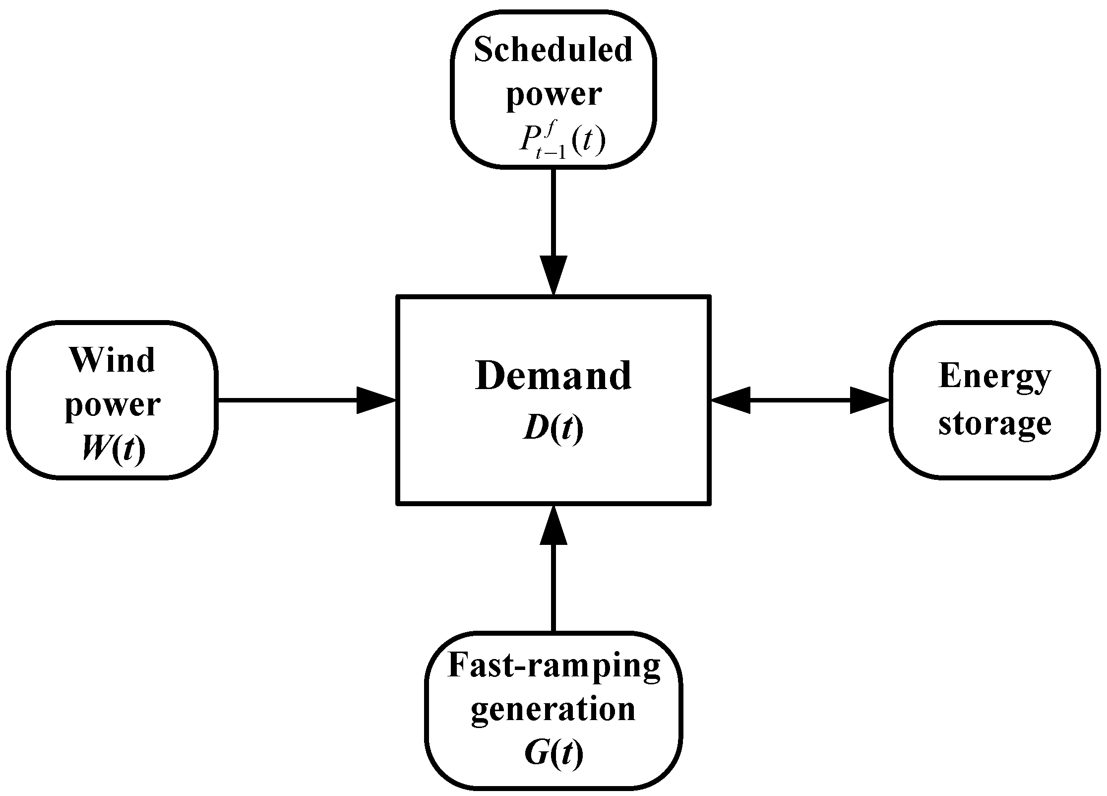
There are four categories of energy sources being used to satisfy the demand in the grid. They are illustrated as follows:

(1)

scheduled power from conventional generators;

(2)

wind power;

(3)

energy storage;

(4)

power from fast-ramping generators.

The demand can always be satisfied via the above energy sources. In real-time scheduling, the system can only modify the output of balance generators to match the demand. The wind power is not dispatchable and is assumed to be free. Also, the fast-ramping generators are mainly gas turbines which are dedicated to compensating for the short time-scale variation in renewable generation [11]. In fact, fast-ramping generation is the reserve of a power system.

Since the wind forecast is inaccurate, the demand probably does not match the combination of scheduled power and wind power at time t. The mismatch will be further balanced with energy storage system and fast-ramping generators. When there is overproduction, the storage will be used to store the excess power. Meanwhile, the storage is first employed to eliminate underproduction. Fast-ramping generation will have to be dispatched if the energy in storage alone is not sufficient to compensate the mismatch. This paper only discusses the case that the storage is concentrated in one place (i.e., there is a single huge storage system).

2.1. Basic Parameters

Similar to literature [12] and [15], a slotted time model is considered, where time is divided into slots whose length are τ. According to the dispatching regulation for power system of China, τ = 15 min in real-time scheduling. It is assumed that power is constant over each time slot, which implies implicitly that the balance of power at time scales shorter than 15 min can be achieved by regulation services, e.g., automatic generation control (AGC). In general, the demand always exceeds the wind production. Figure 1 shows the model of how demand is satisfied by the energy sources aforementioned.

Figure 1. Balancing of demand with different energy sources.

Figure 1. Balancing of demand with different energy sources.

The mismatch M(t) can be denoted as:

$$M(t)=D(t)-W(t)-P_{t-1}^f(t)$$

(1)

η₁ and η₂ account for the losses of energy due to inefficiency of the storage. B_max represents the maximum amount of energy that can be stored. Generally, the energy storage cannot be completely discharged, and there is also a limit on the minimum level. The minimum energy level is taken as a reference and therefore the lower limit is zero. Because of the inefficiency of the storage, the storage system can be charged up to B_max/η₁ units of energy and only produce B_max·η₂ units of energy. B(t) is also referred to as the storage level. B(t) satisfies the constraint B(t) ∈ [0, B_max]. α and β are also known as ramping constraints.

The system operator relies on the wind forecasts to dispatch power from conventional generators. The methodology proposed in this paper does not rely on a particular forecast and it is a general method applying to varieties of wind forecasts. Also, it should be noted that “wind forecast” is used in this paper as a term for forecast of wind power. Load demands, though uncertain, have a statistically predictable aggregate behavior [6]. According to the information provided by State Grid Corporation of China, the forecast error of load is much smaller than that of wind power. Therefore, the demand is assumed to be completely predicable, following [6,10,15]. As a result, the mismatch in Equation (1) is caused only by wind forecast errors.

To evaluate the performance of the proposed scheduling policy in this paper numerically, data from the ERCOT archive is used and this archive is available online at [20].

In real-time scheduling, the wind forecast is provided 15 min ahead. In this timescale, literature [10] observes that the prediction error sequence is independent identically distributed (IID), which indicates that the temporary correlation of the prediction error could be neglected. The 15-min-ahead prediction error ${\mathrm{\epsilon }}_{t-1}^f(t)$ in the ERCOT dataset can be reasonably approximated by Laplace distribution whose probability density function is [1,10]:

$$\Delta (x)=\frac{1}{2}\text{λ}\exp (-\text{λ}|x|)$$

(2)

2.2. Decision Variable, State Variable and State-Transition Function

The existence of storage system would impact real-time scheduling policy, and the real-time scheduling policy could be formulated as follows:

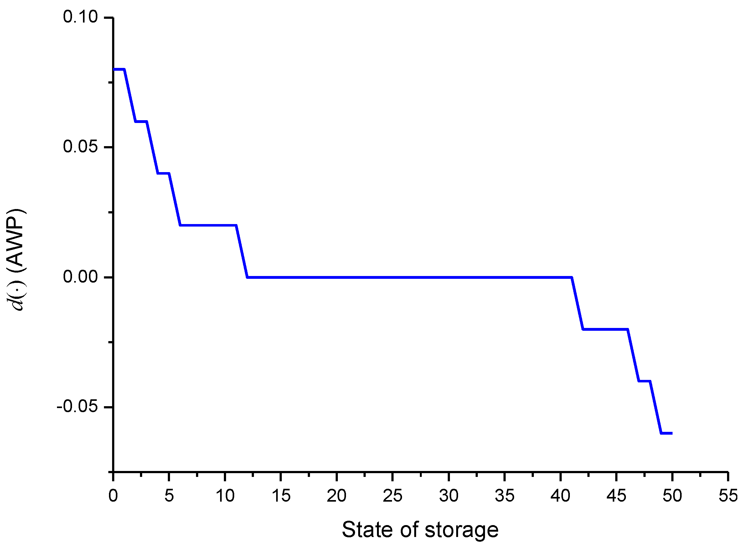
$$P_{t-1}^f(t)=D(t)-W_{t-1}^f(t)+d(B_{t-1}^f(t))$$

(3)

In Equation (3), $d(B_{t-1}^f(t))$ is the additional scheduled power at t that is computed one step ahead. This additional scheduled power is determined according to the forecasted storage level $B_{t-1}^f(t)$. $B_{t-1}^f(t)$ is determined according to B(t − 1), D(t − 1), $W_{t-2}^f(t-1)$, and $P_{t-2}^f(t-1)$. d(•) is a pre-determined function which varies with scheduling policies. This function determines the additional scheduled power from conventional generators according to the forecasted state of storage. Computing function d(•) in Equation (3) is the key step of identifying a scheduling policy and also is the kernel of our scheduling algorithm. For simplicity, a real-time scheduling policy satisfying Equation (3) can be referred to as policy d.

Therefore, function d(•) is the decision variable, and forecasted storage level $B_{t-1}^f(t)$ is the state variable. Energy storage is used to mitigate the mismatch in Equation (1). However, there will be energy loss due to inefficiency of storage cycle, insufficiency of storage capacity and ramping constraints. Fast-ramping generation will be dispatched if the energy in storage alone is not sufficient to compensate the mismatch. Hence, two performance metrics are chosen, namely: (1) the energy loss and (2) the use of fast-ramping generation, which follows the approach in [12] and [15]. Therefore the instantaneous cost C(t) is comprised of these two aspects.

In this paper, the market aspect is ignored, thus the costs of scheduled power from conventional generators and the power from the fast-ramping generators do not vary with time. It is also assumed that the wind energy is free. Under these premises, [10] proves that there exists a stationary greedy storage control strategy that minimizes the expected average magnitude of C(t) under any scheduling policy. Also, this greedy control strategy applies to any form of real-time scheduling policy. The transition function of the greedy control strategy can be described as a unified form:

$$B(t+1)=\varphi (B(t),M(t)\mathrm{\tau })$$

(4)

where:

$$\varphi (B,M\mathrm{\tau })=\{\begin{array}{l}\max (B-\frac{1}{{\mathrm{\eta }}_2}\min (M\mathrm{\tau },\mathrm{\beta }),0) \text{if} M\ge 0,\\ \min (B+{\mathrm{\eta }}_1\min (-M\mathrm{\tau },\mathrm{\alpha }),B_{\max }) \text{if} M<0.\end{array}$$

(5)

Substitute equation Equations (1) and (3) into Equation (4), then Equation (4) becomes:

$$B(t+1)=\varphi (B(t),-{\mathrm{\epsilon }}_{t-1}^f(t)\mathrm{\tau }-d(B_{t-1}^f(t))\mathrm{\tau })$$

(6)

where:

$$B_{t-1}^f(t)=\varphi (B(t-1),(D(t-1)-W_{t-2}^f(t-1)-P_{t-2}^f(t-1))\mathrm{\tau })$$

Equation (6) is the state-transition function. In fact, the state variable $B_{t-1}^f(t)$ has included the status of energy from wind.

According to the IID property of wind forecast errors, Equation (6) has the Markov property, since given the current state, this process’s future behavior is independent of its past history.

If M(t) < 0 and the overproduction cannot be fully injected into the storage system, then the instantaneous cost C(t) is composed of the cost of energy discarding $C_1^d(t)$, and the cost of waste $C_1^w(t)$. If M(t) > 0 and it cannot be fully compensated using the storage, then C(t) is composed of the cost of fast-ramping generation $C_2^f(t)$, and the cost of waste $C_2^w(t)$. Hence, the total instantaneous cost C(t) can be formulated as:

$$C(t)=C_1^d(t)+C_1^w(t)+C_2^w(t)+\text{γ}{C}_2^f(t)$$

(7)

In Equation (4), the first three terms correspond to energy discarding or waste and the last term corresponds to use of fast-ramping generation. The weight coefficient γ represents the trade-off between them. With Equation (4), $C_1^d(t)$, $C_1^w(t)$, $C_2^f(t)$, and $C_2^w(t)$ can be formulated as follows:

$$C_1^d(t)=\max (-M(t)\mathrm{\tau }-\min (\frac{B_{\max }-B(t)}{{\mathrm{\eta }}_1},\mathrm{\alpha }),0)$$

(8)

$$C_1^w(t)=(1-{\mathrm{\eta }}_1)(-M(t)\mathrm{\tau }-C_1^d(t))$$

(9)

$$C_2^f(t)=\max (M(t)\mathrm{\tau }-\min ({\mathrm{\eta }}_{2}B(t),\mathrm{\beta }),0)$$

(10)

$$C_2^w(t)=(\frac{1}{{\mathrm{\eta }}_2}-1)(M(t)\mathrm{\tau }-C_2^f(t))$$

(11)

2.3. Optimization Objectives

Consider a discretized version of the state space of B(t) and the discretized state space is S = {0, 1, 2, ..., B_max/h}. h is the discretization step. There are N_B = 1 + (B_max/h) values in the discretized state space. D_S is the set for decisions.

The reward function f^d of real-time scheduling policy d is defined as follows:

$$f^d(i)=\underset{T\to \infty }{\lim }\frac{{\displaystyle \sum _{t=0}^T}C(t){\text{χ}}_i(t)}{{\displaystyle \sum _{t=0}^T}{\text{χ}}_i(t)}$$

(12)

where i ∈ S. In Equation (12), it should be noted that the storage is operating under the greedy control strategy (Equation (4)). Function χ_i(t) is defined as:

$${\text{χ}}_i(t)=\{\begin{array}{l}1 \text{if} B(t)=i\\ 0 \text{if} B(t)\ne i\end{array}$$

(13)

The long-term behavior of real-time scheduling policy is first going to be optimized. Define the performance measure r^d of policy d which equals to the long-run average of C(t):

$$r^d=\underset{T\to \infty }{\lim }\frac{1}{T}{\displaystyle \sum _{t=0}^{T-1}C(t)}=\underset{T\to \infty }{\lim }\frac{1}{T}{\displaystyle \sum _{t=0}^{T-1}{f}^d(B(t))}$$

(14)

The optimization objective of long-term behavior of real-time scheduling policy is:

$$\underset{d\in D_S}{\min } r^d$$

(15)

D^opt is the set of long-run average cost optimal policies. The elements in D^opt have the same optimal performance measure.

When the parameters of the storage are changed, the corresponding optimal scheduling policy will be different. Since the storage efficiencies will decline because of aging, the system operator will have to replace the optimal scheduling policy with a new one after a period of time. Hence, the short-term behavior of the real-time scheduling policy is also quite important. In this paper, the short-term behavior of the scheduling policy will be further optimized.

Define the bias $g_w^d(i)$ which measures the short-term behavior of policy d starting from state i [21]:

$$g_w^d(i)=\underset{T\to \infty }{\lim }{\displaystyle \sum _{t=0}^{T-1}\{E[f(B(t))-r^d]|B(0)=i\}}$$

(16)

where E(•) is the mathematical expectation. The optimization objective of short-term behavior of the real-time scheduling policy is:

$$\underset{d\in D^{opt}}{\min } g_w^d(i) \text{for} \text{any} i\in S$$

(17)

2.4. Constraints

This paper only deals with the optimization of aggregate output of balance generators. Therefore, only the aggregate power balance constraint is considered here. Though those constraints imposed by the transmission and distribution systems are ignored, our methodology could be extended into a multiple-stage optimization approach to determine the output of each balance generator: First, by calculating the optimal aggregate output of all the balance generators, and then by optimizing the assignment of active power among balance generators with the network constraints. The assignment will not be discussed in this paper.

3. Solution Technique

3.1. Description of Perturbed Markov Decision Process

Literature [21,22,23] provides the sensitivity-based framework of Perturbed MDP. This framework is adopted here as the basis for our policy iteration algorithm. Also, S is the state space of B(t) and D_S is the set for decisions.

In Perturbed Markov decision process, Equation (15) is equivalent to (see [21], Chapter 4):

$$\underset{d\in D_S}{\min } f^d(i)+{\displaystyle \sum _{j\in S}}{P}^d(j|i)g^d(j) \text{for} \text{any} i\in S$$

(18)

where g^d is the performance potential of policy d and P^d is the transition matrix of policy d.

Define the bias $g_w^d$ of policy d which measures the short-term behavior of d:

$$g_w^d=[{(I-P^d+e{\text{π}}^d)}^{-1}-e{\text{π}}^d]f^d$$

(19)

where π^d is the steady-state probabilities of the Markov chain under policy d, f^d = (f(1), f(2), ..., f(N_B))^T, e is a 1-by-N_B vector and e = (1, 1,..., 1)^T, I is the identity matrix of order N_B.

In Perturbed MDP, Equation (17) is equivalent to (see [21], Chapter 4):

$$\underset{d\in D^{opt}}{\min } P^d{w}^d$$

(20)

where w^d is the bias-potential of policy d.

3.2. Linearization Approximation

Substitute Equation (3) into Equation (1), then the following equation is obtained

$$M(t)=-{\mathrm{\epsilon }}_{t-1}^f(t)-d(B_{t-1}^f(t))$$

(21)

Because:

$$\begin{array}{l}B(t)=\varphi (B(t-1),D(t-1)\mathrm{\tau }-W(t-1)\mathrm{\tau }-P_{t-2}^f(t-1)\mathrm{\tau })\\ =\varphi (B(t-1),D(t-1)\mathrm{\tau }-W_{t-2}^f(t-1)\mathrm{\tau }-P_{t-2}^f(t-1)\mathrm{\tau }-{\mathrm{\epsilon }}_{t-2}^f(t-1)\mathrm{\tau })\\ B^f(t)=\varphi (B(t-1),D(t-1)\mathrm{\tau }-W_{t-2}^f(t-1)\mathrm{\tau }-P_{t-2}^f(t-1)\mathrm{\tau })\end{array}$$

thus:

$$\begin{array}{l}B(t)=\min (B_{t-1}^f(t)+{\mathrm{\epsilon }}_{t-2}^f(t-1)\mathrm{\tau },B_{\max }/h)+\max (B_{t-1}^f(t)+{\mathrm{\epsilon }}_{t-2}^f(t-1)\mathrm{\tau },0)\\ -(B_{t-1}^f(t)+{\mathrm{\epsilon }}_{t-2}^f(t-1)\mathrm{\tau })\end{array}$$

(22)

Substitute Equation (22) into Equation (21), and Equation (21) becomes:

$$M(t)\approx -{\mathrm{\epsilon }}_{t-1}^f(t)-d(B(t)-{\mathrm{\epsilon }}_{t-2}^f(t-1)\mathrm{\tau })$$

(23)

In Equation (23), the border conditions on B(t) is neglected since ${\mathrm{\epsilon }}_{t-2}^f(t-1)\mathrm{\tau }$ is quite small [1,10]. Replace M(t) in Equation (4) with Equation (23), then:

$$B(t+1)=\varphi (B(t),-{\mathrm{\epsilon }}_{t-1}^f(t)\mathrm{\tau }-d(B(t)-{\mathrm{\epsilon }}_{t-2}^f(t-1)\mathrm{\tau })\mathrm{\tau })$$

(24)

In fact, the forecast error in the timescale of real-time scheduling is so small that $d(B(t)-{\epsilon }_{t-2}^f(t-1)\mathrm{\tau })$ can be linearized near B(t) and the following equation is obtained:

$$d(B(t)-{\mathrm{\epsilon }}_{t-2}^f(t-1)\mathrm{\tau })\approx d(B(t))-{\mathrm{\epsilon }}_{t-2}^f(t-1)$$

(25)

Therefore, Equation (24) becomes:

$$B(t+1)=\varphi (B(t),{\mathrm{\epsilon }}_{t-2}^f(t-1)\mathrm{\tau }-{\mathrm{\epsilon }}_{t-1}^f(t)\mathrm{\tau }-d(B(t))\mathrm{\tau })$$

(26)

The approximation in Equation (26) is quite essential for the policy optimization method that will be developed below, since it erases the correlations between the actions in different states of B(t). With this special property, the function d(•) can be derived with policy iteration approach.

3.3. The Policy Iteration Algorithm

For simplicity, the following equations are defined:

$$\overline{i}=\min (i+\frac{\mathrm{\alpha }}{h},\frac{B_{\max }}{h})$$

(27)

$$\underset{¯}{i}=\max (i-\frac{\mathrm{\beta }}{h},0)$$

(28)

$${\Delta }_{\tau }(x,i)=\Delta (\frac{60}{\mathrm{\tau }}[x-(ih+d(i)\mathrm{\tau })])$$

(29)

$${\Delta }^d(x,i)={\displaystyle {\int }_{-\infty }^{+\infty }{\Delta }_{\tau }(\text{ζ},i)}{\Delta }_{\tau }(-x+\text{ζ},i) d\text{ζ}$$

(30)

where i ∈ S, h is the discretization step. It should be noted that Equation (30) is based on the IID assumption of wind forecast error. If this assumption does not hold, Δ^d(x,i) will have to be formulated in a different way. However, the algorithms introduced below apply to any form of Δ^d(x,i).

Then, the transition matrix under policy d is formulated as:

$$P^d(i,j)=\{\begin{array}{l}{\displaystyle {\int }_{jh-\frac{1}{2}h}^{+\infty }} {\Delta }^d (x,i) dx \text{if} j=\overline{i}\\ {\displaystyle {\int }_{-\infty }^{jh+\frac{1}{2}h}} {\Delta }^d (x,i) dx \text{if} j=\underset{¯}{i}\\ {\displaystyle {\int }_{jh-\frac{1}{2}h}^{jh+\frac{1}{2}h}} {\Delta }^d (x,i) dx \text{if} \underset{¯}{i}<j<\overline{i}\\ 0 \text{otherwise}\end{array}$$

(31)

where j ∈ S and the corresponding reward function is:

$$\begin{array}{l}{f}^d(i)\\ ={\displaystyle {\int }_{-\infty }^{\underset{¯}{i}h}}(\gamma (\underset{¯}{i}h-x)+(\frac{1}{{\eta }_2}-1)(ih-\underset{¯}{i}h)){\Delta }^d(x,i) dx\\ +{\displaystyle {\int }_{\underset{¯}{i}h}^{ih}}(\frac{1}{{\eta }_2}-1)(ih-x){\Delta }^d(x,i) dx\\ +{\displaystyle {\int }_{ih}^{\overline{i}h}}(1-{\eta }_1)(x-ih){\Delta }^d(x,i) dx\\ +{\displaystyle {\int }_{\overline{i}h}^{+\infty }}((x-\overline{i}h)+(1-{\eta }_1)(\overline{i}h-ih)){\Delta }^d(x,i) dx\end{array}$$

(32)

Equations (31) and (32) are derived with Equation (26) and Equations (8)–(11).

The policy iteration algorithm proposed for deriving optimal real-time scheduling policy is composed of three sub-algorithms, namely Algorithm 1, Algorithm 2 and Algorithm 3.

Algorithm 1 provides an efficient way to numerically compute performance potential g^d of policy d. Algorithm 2 searches for the policy d that minimizes long-term performance measure r^d corresponding to Equation (15) and identifies the set D^opt. In Algorithm 3, the Bias-Optimal policy that has the optimal short-term behavior corresponding to Equation (17) is selected in the elements of set D^opt.

The proposed policy iteration algorithm has a two-level optimization structure since Algorithm 3 is based on the output of Algorithm 2: Equation (15) is the upper-level optimization while Equation (17) is the lower-level one. Figure 2 shows the two-level optimization structure of policy iteration algorithm.

Figure 2. Two-level optimization structure of policy iteration algorithm.

Figure 2. Two-level optimization structure of policy iteration algorithm.

Algorithm 1, Algorithm 2 and Algorithm 3 are shown as follows.

Algorithm 1 Computation of gd

k←0; g0(i) ←0 for all i ∈ S; Step 1) Pd←Pd-ep* (p* is the NB th row of Pd) fd←fd-e fd(NB) k←k+1; gk←fd; Step (2) While supi |gk(i)-gk-1(i)| ≥ precision threshold do k←k+1; gk←fd+ Pd gk-1 End while Step (3) gd(i) ←gk(i) for all i ∈ S

Algorithm 2 Computation of the set of long-run average cost optimal policies

v ←0; d0(i) ←0 for all i ∈ S; ξ←1; Di = ∅ for all i ∈ S Step (1) Input: weight coefficient γ, discretization step h, probability density function Δ. Step (2) While ξ ≠ 0 do Compute $g^{d_v}$ using Algorithm 1 Choose: $d_{v+1}(i)\in \arg \{\underset{u\in A}{\min }[f^u(i)+{\displaystyle \sum _{j\in S}{P}^u(j|i)g^{d_v}(j)}]\}$ for all i ∈ S ξ←supi|dv+1(i) − dv(i)|; v ←v+1; End while Step (3) $\begin{array}{l}{D}_i=\{u\in A:f^u(i)+{\displaystyle \sum _{j\in S}{P}^u(j|i)g^{d_v}(i)}\\ =f^{d_v}(i)+{\displaystyle \sum _{j\in S}{P}^{d_v}(j|i)g^{d_v}(i)}\}\end{array}$ Dopt = X i ∈ S Di

In Algorithm 2 above, “X” is called Cartesian product, which is a direct product of sets.

Algorithm 3 Policy iteration algorithm for Bias-Optimal policy

v ←0; ξ←1; Step (1) Compute Dopt using Algorithm 2 select any d0∈ Dopt Step (2) While ξ ≠ 0 do Compute bias $g_w^{d_v}$ using Equation (19) $w^{d_v}=-{(I-P^{d_v})}^{-1}{g}_w^{d_v}$ Choose: $d_{v+1}\in \arg \{\underset{u\in D^{opt}}{\min }[P^u{w}^{d_v}]\}$ ξ←supi|dv+1(i) − dv(i)|; v ←v+1; End while Step (3) d(i)=dv(i) for all i ∈ S

The function d obtained in Algorithm 3 is the Bias-Optimal policy which is also a long-run average cost optimal policy. It is employed as the real-time scheduling policy. The system operator can determine the aggregate power $P_{t-1}^f(t)$ scheduled from conventional generators for the next step using the derived function d(•), Equation (3) and wind forecast.

In the multi-time scale coordinated active power scheduling framework, the output of base load power plants and part of intermediate power plants are fixed after rolling scheduling is activated. In real-time scheduling, the optimal aggregate output of balance generators is equal to the difference between the renewed $P_{t-1}^f(t)$ and those with fixed power output:

$$P_{\text{bal}}^f(t)=P_{t-1}^f(t)-P_{\text{fix}}^{rt}(t)$$

(33)

where $P_{\mathrm{bal}}^f(t)$ is the optimal aggregate output of balance generators at t, and $P_{\mathrm{fix}}^{rt}(t)$ is the fixed power output in the system in real-time scheduling at t.

4. Numerical Example

4.1. Parameter Setting

The ERCOT archive provides aggregate electricity production, demand as well as wind output in Texas. The data are sampled every 5 min, and they are used to obtain the 15 min average values.

All units in this paper will be normalized with average wind power (AWP). 1 AWP is equal to the average over time of W(t) in ERCOT archive. In this normalization, the unit AWPh corresponds to the average wind energy generated during one hour. The aggregate wind capacity in Texas is 12,000 MW and the average output is approximately 3000 MW. Hence, 1 AWP equals 3000 MW and 1 AWPh is equivalent to 3000 MWh.

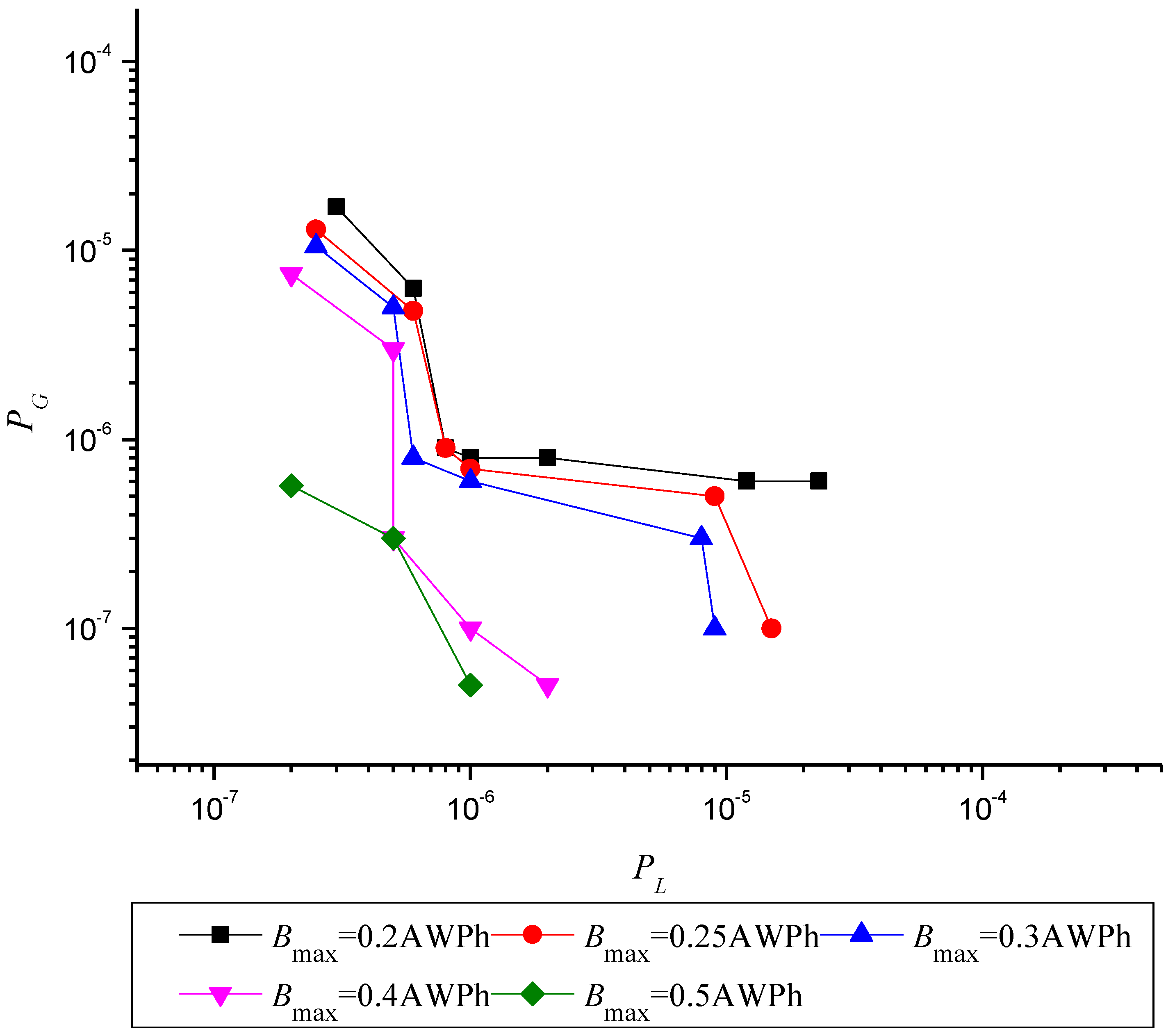
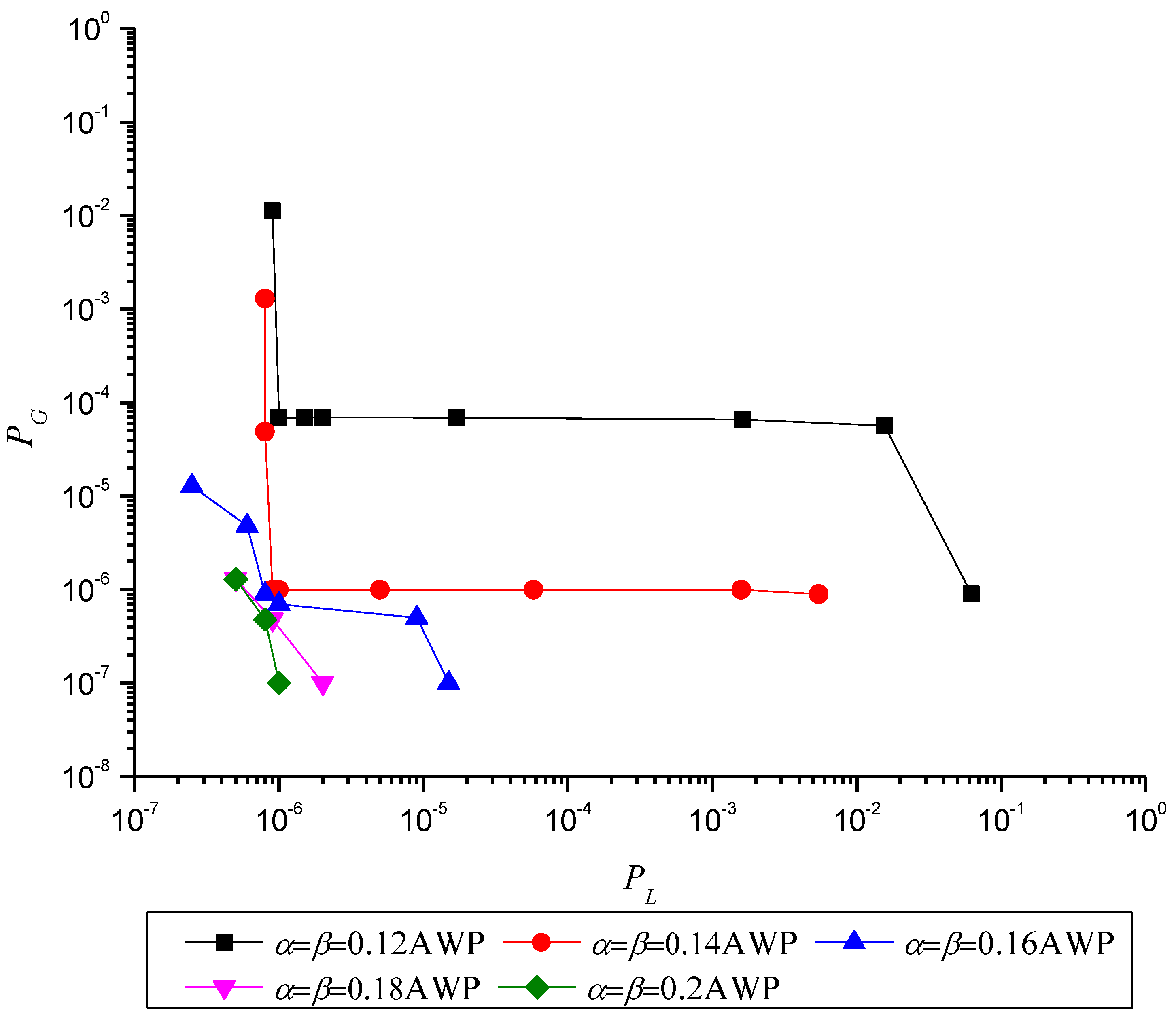
The storage system has a capacity of 0.25 AWPh. Both the efficiency of charging process and discharging process of the storage are 0.9 (i.e., η₁ = η₂ = 0.9). The ramping constraints are α = β = 0.16 AWP. The parameter λ of the best fit Laplace distribution of 15-min-ahead prediction error for the ERCOT dataset is 38.22.

4.2. Verification of Long-Term Performance of Policy Iteration Algorithm

An illustration of function d(•) of the real-time scheduling policy obtained with the parameters in Section 4.1 is shown in Figure 3. Set discretization step h = 0.005 AWPh, which means the state space of storage is {0, 1, 2,..., 50}. Weight coefficient γ is set at 2.

The long-term performance of the real-time scheduling policy in Figure 3 can be represented by a point (P_L, P_G), where P_L is the probability of energy discarding and P_G is the probability of use of fast-ramping generation. P_L and P_G can be calculated by Monte Carlo simulation of that scheduling policy. For the policy in Figure 3, the values of P_L and P_G are equal to 10⁻⁶ and 7 × 10⁻⁷, respectively. Hence, the point is (10⁻⁶, 7 × 10⁻⁷). If γ is varied from 0.01 to 100, this point will evolve into a curve. This curve measures the long-term performance of policy iteration algorithm under the parameter setting in Section 4.1. When γ is larger than 1, the algorithm gives more importance to the cost of fast-ramping generation. Since fast-ramping generators are very costly to operate and produce environmentally harmful emissions, the system operator in China is much more concerned about the use of fast-ramping generators. Therefore, the part of the curve which corresponds to γ > 1 is paid more attention.

The curve can be drawn on a coordinate plane whose horizontal axis is P_L and vertical axis is P_G. The origin (0,0) is the point that represents the idealistic scenario where no energy discarding or use of fast-ramping generation takes place. The closer the curve lies to the origin, the better the long-term performance of algorithm is.

Figure 3. Derived real-time scheduling policy.

Figure 3. Derived real-time scheduling policy.

4.2.1. Long-Term Performance of Policy Iteration Algorithm within Various Storage Parameters

The capacity, ramping constraints as well as the efficiencies of the storage system could influence the discarding energy [24] or the use of fast-ramping generation and thus the long-term performance of the policy iteration algorithm.

In order to study the influence of storage capacity on policy iteration algorithm, set the storage capacity at B_max = 0.2 AWPh, B_max = 0.25 AWPh, B_max = 0.3 AWPh, B_max = 0.4 AWPh, B_max = 0.5 AWPh respectively, while the ramping constraints, efficiencies of storage and wind forecast remain unchanged. The long-term performances of policy iteration algorithm in these cases are drawn in Figure 4. γ is varied from 0.01 to 100.

In Figure 4, the values of the two considered metrics (P_L and P_G) of all the curves are always kept at low levels. And when B_max is less than 0.3 AWPh, there is nuance of position between the corresponding curves. Thus, the policy iteration algorithm operates effectively.

Previously, in China the typical capacity of a storage system that is designed to compensate for the short term uncertainty (15 min–1 h) of wind power is more than 0.8 AWPh. Moreover, the wind forecasting error currently averages at 3%–5% (root mean square error) of the capacity of wind farm for an hour-ahead forecast, and reduces progressively to 1%–2% for 15 min-ahead forecast. Since the proposed algorithm is still competent when B_max = 0.25 AWPh (with 15 min-ahead forecast), the work in this paper does reduce the capacity of storage that is needed to mitigate wind fluctuation in active power dispatching. Furthermore, the forecasting error of 15 min-ahead forecast could be up to 0.12 AWP (equal to 0.03 AWPh in terms of energy), which accounts for 12% (>10%) of the chosen storage capacity (0.25 AWPh). Further, because of the inefficiency of the storage, the storage system can only produce B_max·η₂ units of energy. Therefore, the result that the policy iteration algorithm behaves well when B_max = 0.25 AWPh reveals its competence.

Figure 4. Long-term performance of policy iteration algorithm under different storage capacities.

Figure 4. Long-term performance of policy iteration algorithm under different storage capacities.

Set the ramping constraints at α = β = 0.12 AWP, α = β= 0.14 AWP, α = β = 0.16 AWP, α = β = 0.18 AWP, α = β = 0.2 AWP, respectively, while the rest of the parameters of storage as well as the wind forecast are kept the same with those in Section 4.1. The long-term performances of the proposed algorithm in these cases are drawn in Figure 5. γ is varied from 0.01 to 100.

When ramping constraints α and β are greater than 0.16 AWP, the corresponding curves in Figure 5 lie in a narrow area near the origin, which reveals the competence of the algorithm. However, in Figure 5, P_L and P_G vary drastically when α and β are less than 0.16 AWP. This phenomenon is brought about by the inaccuracy of wind forecast and relative lack of ramping capability of the storage. Yet, in practice, the ramping capability of storage is always sufficient enough to ensure the good long-term performance of the policy iteration algorithm, see [8].

Eight pairs of charging process efficiency η₁ and discharging process efficiency η₂ are chosen, namely η₁ = 1 and η₂ = 1, η₁ = 0.9 and η₂ = 0.9, η₁ = 0.9 and η₂ = 0.8, η₁ = 0.8 and η₂ = 0.8, η₁ = 0.7 and η₂ = 0.8, η₁ = 0.6 and η₂ = 0.8, η₁ = 0.6 and η₂ = 0.5, η₁ = 0.6 and η₂ = 0.4. For each pair of efficiencies, γ is varied from 0.01 to 100 while the storage capacity is kept at 0.25 AWPh and ramping constraints remain at α = β = 0.16 AWP. Also, the wind forecast is kept the same with that in Section 4.1.

Two important observations are made from Figure 6. First, when the cycle efficiency (product of η₁ and η₂) of the storage is above 0.6, P_L or P_G are all below 10⁻³, which implies that the long-term performance of the policy iteration algorithm is pretty well within a large range of cycle efficiency. Second, when the cycle efficiency of the storage is above 0.4 and γ is above 1, the probabilities of use of fast-ramping generation are all below 10⁻⁵, which indicates that the policy iteration algorithm can reduce the capacity of fast-ramping generation (the reserve of a system) to a great extent.

Apparently, the probabilities of energy discarding or the use of fast-ramping generation tend to decrease when the storage capacity increases, ramping constraints are extended, or the efficiencies are raised.

Figure 5. Long-term performance of policy iteration algorithm under different ramping constraints.

Figure 5. Long-term performance of policy iteration algorithm under different ramping constraints.

Figure 6. Long-term performance of policy iteration algorithm under different storage efficiencies.

Figure 6. Long-term performance of policy iteration algorithm under different storage efficiencies.

4.2.2. Long-Term Performance of Policy Iteration Algorithm under Various Wind Forecasts

The parameter λ represents the accuracy of the wind forecast: the greater the λ, the more accurate the forecast. In order to study the long-term performance of proposed algorithm under wind forecasts of different accuracies, four different wind forecasts are chosen whose λ are 31.43, 38.22, 47.14, and 56.47, respectively. These different wind forecasts are chosen from different wind databases and hence they have different forecast accuracies. The parameters of storage are kept the same with those in Section 4.1. The long-term performances of the proposed algorithm are shown in Figure 7. γ is varied from 0.01 to 100.

As shown in Figure 7, the policy iteration algorithm performs better with the better (more accurate) wind forecast. In fact, Figure 4, Figure 5, Figure 6 and Figure 7 reveal the consistency of the proposed policy iteration algorithm: Better storage parameters or better wind forecasts result in a better long-term performance of the algorithm.

Figure 7. Long-term performance of policy iteration algorithm under different wind forecasts.

Figure 7. Long-term performance of policy iteration algorithm under different wind forecasts.

4.3. Verification of Short-Term Performance of Policy Iteration Algorithm

The short-term performance of a real-time scheduling policy can be measured by its bias. In order to compute bias numerically, Equation (20) can be rewritten as:

$$g_w^d(i)=\underset{T\to \infty }{\lim }{\displaystyle \sum _{t=0}^{T-1}}\{E[f(B(t))-r^d]|B(0)=i\} \text{for} \text{any} i\notin S$$

where B(t) is the state of storage at time t, and E(•) is mathematical expectation. The Monte Carlo simulation is used to compute Equation (16). For convenience, B(0) is set at 0. For simplicity, the cost is normalized: The cost of 1 AWPh energy discarding is 1.

Two policies are compared in Figure 8, namely d_ite obtained with the policy iteration algorithm proposed in this paper and d_off obtained with dynamic offset policy in [15]. These two policies are derived with the same parameter setting in Section 4.1 and γ = 2. They have the same optimal long-run average cost. According to Equation (16), the bias of a policy is equal to the area of the region bounded by the curve, the dashed line and the vertical axis. The smaller the area is, the lower the short-term cost is.

It can be seen in Figure 8 that the area bounded by d_ite is less than that bounded by d_off. Hence, the policy iteration algorithm proposed in this paper outperforms the dynamic offset policy of [15] in short-term performance.

Figure 8. Comparison of short-term performance of policies derived with different method.

Figure 8. Comparison of short-term performance of policies derived with different method.

4.4. Performance of Policy Iteration Algorithm under Different Discretization Steps

Intuitively, the capacity of the storage system will influence the choice of discretization step. Therefore, five storage capacities for test are chosen, namely B_max = 0.2 AWPh, B_max = 0.25 AWPh, B_max = 0.3 AWPh, B_max = 0.4 AWPh and B_max = 0.5 AWPh. Each of the test capacities is simulated in four discretization steps, namely h = 0.001 AWPh, h = 0.005 AWPh, h = 0.01 AWPh and h = 0.02 AWPh. The rest of the parameters of storage and wind forecast are kept the same with those in Section 4.1.

The long-term performance of policy iteration algorithm corresponding to each capacity of storage under different discretization steps is drawn in Figure 9 (γ is varied from 0.01 to 100).

The performance of the policy iteration algorithm corresponding to each discretization step is scarcely sensitive to the capacity of storage, which reveals the robustness of the proposed algorithm—the performance of an algorithm under a particular discretization step is hardly influenced by the scale of the problem. The probabilities of energy discarding or the use of fast-ramping generation when h = 0.01 AWPh or h = 0.02 AWPh are relatively much greater, while the probabilities are all less than 2 × 10⁻⁵ when h = 0.001 AWPh or h = 0.005 AWPh. Furthermore, there is only minute difference between the performances corresponding to h = 0.005 AWPh and h = 0.001 AWPh.

Figure 9. Performance of policy iteration algorithm under different discretization steps and storage capacities.

Figure 9. Performance of policy iteration algorithm under different discretization steps and storage capacities.

Table 1 lists the number of iterations and computational time of the proposed algorithm under different discretization steps and storage capacities. The program is run on a desktop PC with an Inter^® Core™ i5-2430M 2.40 GHz CPU, and 4 GB Samsung/1333 RAM.

Table 1. Number of iterations and computational time of the proposed algorithm under different discretization steps and storage capacities.

Bmax (AWPh)		h = 0.001 AWPh	h = 0.005 AWPh	h = 0.01 AWPh	h = 0.02 AWPh
0.2	Iteration	12	7	6	4
	Time(s)	0.57	0.21	0.011	0.010
0.25	Iteration	12	7	6	4
	Time(s)	0.68	0.24	0.016	0.013
0.3	Iteration	12	8	6	4
	Time(s)	0.89	0.35	0.093	0.018
0.4	Iteration	12	8	6	4
	Time(s)	1.45	0.49	0.10	0.03
0.5	Iteration	12	9	7	5
	Time(s)	1.53	0.87	0.27	0.04

Table 1. Number of iterations and computational time of the proposed algorithm under different discretization steps and storage capacities.

Bmax (AWPh)		h = 0.001 AWPh	h = 0.005 AWPh	h = 0.01 AWPh	h = 0.02 AWPh
0.2	Iteration	12	7	6	4
	Time(s)	0.57	0.21	0.011	0.010
0.25	Iteration	12	7	6	4
	Time(s)	0.68	0.24	0.016	0.013
0.3	Iteration	12	8	6	4
	Time(s)	0.89	0.35	0.093	0.018
0.4	Iteration	12	8	6	4
	Time(s)	1.45	0.49	0.10	0.03
0.5	Iteration	12	9	7	5
	Time(s)	1.53	0.87	0.27	0.04

Though the number of iterations and computational time are affected by the discretization step and capacity of the storage, the number of iterations required is moderate and the computational time is also acceptable. Give consideration to both the performance of algorithm and computational burden, the appropriate discretization step should be h = 0.005 AWPh or h = 0.001 AWPh, which applies to a wide range of storage capacities. Also, it is reasonable to claim that the policy iteration algorithm has good convergence and high computational efficiency.

5. Conclusions

In order to tackle the scheduling problem in the wind-connected system presented with storage and wind forecast uncertainties, the energy loss and use of fast-ramping generation are chosen as the performance metrics. The policy iteration algorithm is developed to compute the real-time scheduling policy that is both long-run average cost optimal and bias-optimal. The algorithm is derived with Perturbed Markov decision process. The optimal aggregate output of balance generators is obtained with this scheduling policy. Also, the optimal storage control strategy that is tightly coupled with the real-time scheduling policy is described. The proposed algorithm for real-time scheduling is evaluated with real data in the ERCOT dataset. The results of numerical experiments reveal that the algorithm can reduce the energy loss and use of fast-ramping generation to a great extent. Also, the short-term and long-term performance of the proposed algorithm is verified and the consistency, robustness, good convergence and high computational efficiency of the algorithm are corroborated by varying a number of different parameters.

It should be noted that real-time scheduling and storage control are just part of the multi-time scale coordinated active power scheduling framework. Our subsequent studies will be concentrated on the remainder of the multi-time scale coordinated active power scheduling framework. It is very interesting to explore the case when the storages are distributed. We also want to extend our framework into market environments and other types of renewable power generation.

References

1. Hodge, B.; Milligan, M. Wind power forecasting error distributions over multiple timescales. In Proceedings of the IEEE Power and Energy Society General Meeting, San Diego, CA, USA, 21–24 August 2011.
2. Zhang, Z.-S.; Sun, Y.-Z.; Gao, D.W.; Jin, L.; Lin, C. A versatile probability distribution model for wind power forecast errors and its application in economic dispatch. IEEE Trans. Power Syst. 2013, 28, 3114–3125. [Google Scholar] [CrossRef]
3. Wu, W.; Zhang, B.; Chen, J.; Zhen, T. Multiple time-scale coordinated power control system to accommodate significant wind power penetration and its real application. In Proceedings of the IEEE Power and Energy Society General Meeting, San Diego, CA, USA, 22–26 July 2012.
4. Zhang, B.; Wu, W.; Zheng, T.; Sun, H. Design of a multi-time scale coordinated active power dispatching system for accommodating large scale wind power penetration. Autom. Electr. Power Syst. 2011, 35, 1–6. [Google Scholar]
5. Li, Z.; Zhang, B.; Wu, W.; Sun, H.; Guo, Q. Dynamic economic dispatch using lagrangian relaxation with multiplier updates based on a quasi-newton method. IEEE Trans. Power Syst. 2013, 28, 4516–4527. [Google Scholar] [CrossRef]
6. Varaiya, P.P.; Wu, F.F.; Bialek, J.W. Smart operation of smart grid: Risk-limiting dispatch. IEEE Proc. 2011, 99, 40–57. [Google Scholar] [CrossRef]
7. Hetzer, J.; Yu, D.C.; Bhattarai, K. An economic dispatch model incorporating wind power. IEEE Trans. Energy Convers. 2008, 23, 603–611. [Google Scholar] [CrossRef]
8. Chen, C.; Lee, T.; Jan, R. Optimal wind-thermal coordination dispatch in isolated power systems with large integration of wind capacity. Energy Convers. Manag. 2006, 47, 3456–3472. [Google Scholar] [CrossRef]
9. Divya, K.C.; Østergaard, J. Battery energy storage technology for power systems—An overview. Electric Power Syst. Res. 2009, 79, 511–520. [Google Scholar] [CrossRef]
10. Han-I, S.; El Gamal, A. Modeling and analysis of the role of energy storage for renewable integration: Power balancing. IEEE Trans. Power Syst. 2013, 28, 4109–4117. [Google Scholar] [CrossRef]
11. Han-I, S.; El Gamal, A. Modeling and analysis of the role of fast-response energy storage in the smart grid. In Proceedings of the 49th Annual Allerton Conference, Monticello, IL, USA, 28–30 September 2011.
12. Bejan, A.; Gibbens, R.; Kelly, F. Statistical aspects of storage systems modelling in energy networks. In Proceedings of the 46th Annual Conference on Information Sciences and Systems, Princeton, NJ, USA, 21–23 March 2012.
13. Yao, D.L.; Choi, S.S.; Tseng, K.J.; Lie, T.T. Determination of short-term power dispatch schedule for a wind farm incorporated with dual-battery energy storage scheme. IEEE Trans. Sustain. Energy 2012, 3, 74–84. [Google Scholar] [CrossRef]
14. Nascimento, J.; Powell, W.B. An optimal approximate dynamic programming algorithm for concave, scalar storage problems with vector-valued controls. IEEE Trans. Autom. Control 2013, 58, 2995–3010. [Google Scholar] [CrossRef]
15. Gast, N.; Tomozei, D.C.; Le, J.Y. Boudec, optimal generation and storage scheduling in the presence of renewable forecast uncertainties. IEEE Trans. Smart Grid 2014, 5, 1328–1339. [Google Scholar] [CrossRef]
16. Miao, H.; Murugesan, S.; Junshan, Z. A multi-timescale scheduling approach for stochastic reliability in smart grids with wind generation and opportunistic demand. IEEE Trans. Smart Grid 2013, 4, 521–529. [Google Scholar] [CrossRef]
17. Leterme, W.; Ruelens, F.; Claessens, B.; Belmans, R. A flexible stochastic optimization method for wind power balancing with PHEVs. IEEE Trans. Smart Grid 2014, 5, 1238–1245. [Google Scholar] [CrossRef]
18. Junseok, S.; Krishnamurthy, V.; Kwasinski, A.; Sharma, R. Development of a Markov-chain-based energy storage model for power supply availability assessment of photovoltaic generation plants. Trans. IEEE Sustain. Energy 2013, 4, 491–500. [Google Scholar] [CrossRef]
19. Luh, P.B.; Yu, Y.; Zhang, B.; Litvinov, E.; Zheng, T.; Zhao, J.; Wang, C. Grid integration of intermittent wind generation: A Markovian approach. IEEE Trans. Smart Grid 2014, 5, 732–741. [Google Scholar] [CrossRef]
20. Grid Information. Available online: http://www.ercot.com/gridinfo (accessed on 5 September 2014).
21. Cao, X.-R. Stochastic Learning and Optimization: A Sensitivity-Based View; Springer: Heidelberg, Germany, 2007. [Google Scholar]
22. Liu, K. Perturbed Markov Decision Processes and Hamiltonian Cycles; University of Science and Technology of China Press: Hefei, China, 2009. [Google Scholar]
23. Puterman, M. Markov Decision Processes: Discrete Stochastic Dynamic Pogramming; Wiley: New York, NY, USA, 1994. [Google Scholar]
24. Xi, X.; Sioshansi, R. A stochastic dynamic programming model for co-optimization of distributed energy storage. Energy Syst. 2014, 5, 474–505. [Google Scholar] [CrossRef]