Application Study on the Dynamic Programming Algorithm for Energy Management of Plug-in Hybrid Electric Vehicles

Abstract

To explore the problems associated with applying dynamic programming (DP) in the energy management strategies of plug-in hybrid electric vehicles (PHEVs), a plug-in hybrid bus powertrain is introduced and its dynamic control model is constructed. The numerical issues, including the discretization resolution of the relevant variables and the boundary issue of their feasible regions, were considered when implementing DP to solve the optimal control problem of PHEVs. The tradeoff between the optimization accuracy when using the DP algorithm and the computational burden was systematically investigated. As a result of overcoming the numerical issues, the DP-based approach has the potential to improve the fuel-savings potential of PHEVs. The results from comparing the DP-based strategy and the traditional control strategy indicate that there is an approximately 20% improvement in fuel economy.

1. Introduction

In contrast to hybrid electric vehicles (HEVs), plug-in hybrid electric vehicles (PHEVs) have a larger battery, which can replace a certain amount of conventional fossil fuels with grid electricity [1,2,3,4]. The manner in which the onboard electrical energy is used significantly influences the energy utilization efficiency and subsequently impacts the fuel economy [5,6,7,8].

As an approach that solves multi-step optimization problems based on Bellman’s principle of optimality [9,10], dynamic programming (DP) guarantees global optimality through an exhaustive search of all control and state grids. Applying DP in PHEVs consists of finding optimal control sequences to obtain the optimal battery state of charge (SoC) trajectory and to minimize fuel consumption over a given driving schedule. The DP-based energy management strategy belongs to the category of off-line energy management techniques, which are not suitable for online control [11]. However, this approach provides a benchmark for assessing the optimality of other energy management strategies and helps to improve the online strategy [12,13,14,15,16].

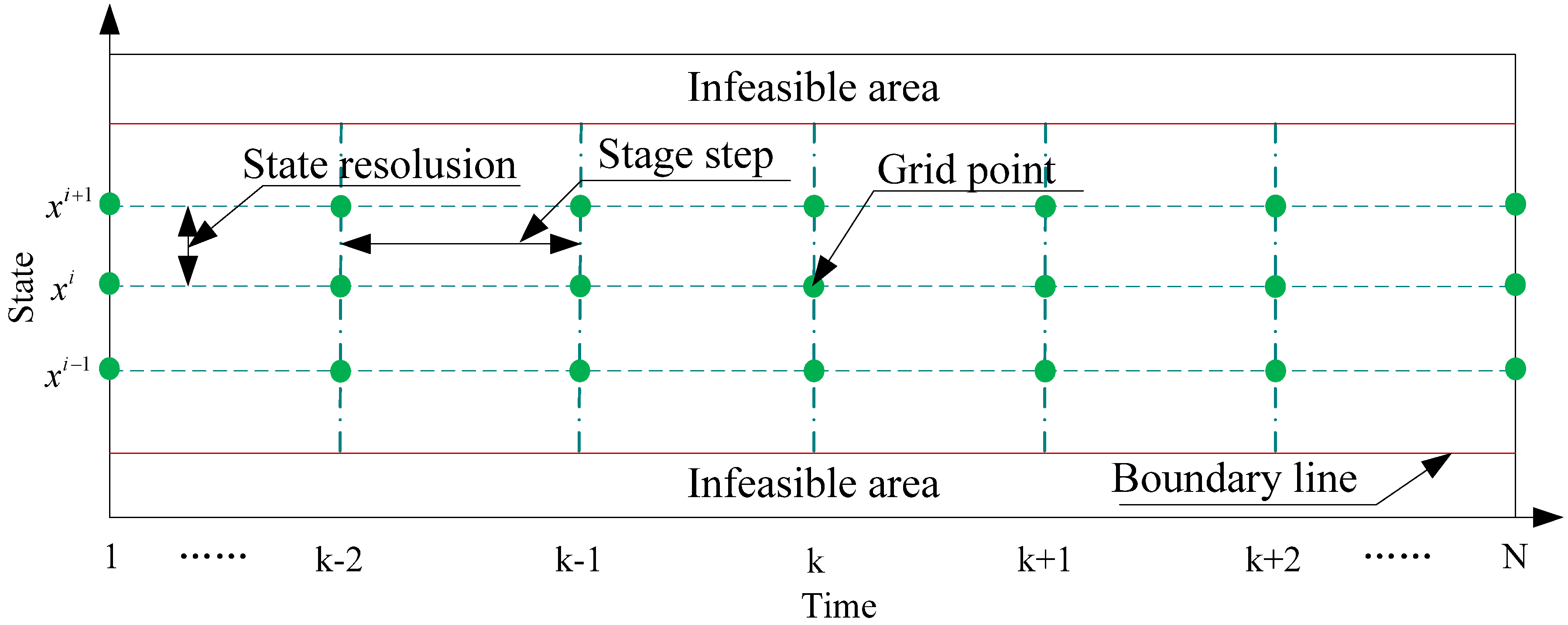
Because DP is a numerical algorithm, the continuous-time control problem must be discretized. In fact, the DP processes are implemented backward from the final state to the initial state by searching for the optimal trajectory among the discretized grid points. Moreover, the grid points are the intersections of discretizing lines of state space and time space, as shown in Figure 1. However, the state output of the model function is continuous in the state space, which does not generally coincide with the nodes of the state grid but rather between them. Consequently, it is necessary to appropriately evaluate the DP process, and interpolation is used to find the cost-to-go value, which inherently introduces numerical errors [17,18]. Therefore, the accuracy of the DP solutions depends on the number of grid points [19]. Higher discretization resolution of the state space and time space could increase the number of grid points, which would consequently increase the optimality of the DP results. Unfortunately, higher discretization resolution also leads to an increase in the computation load required to calculate the global optimum [17,19,20].

Figure 1. Discretization of the state space and time space.

Figure 1. Discretization of the state space and time space.

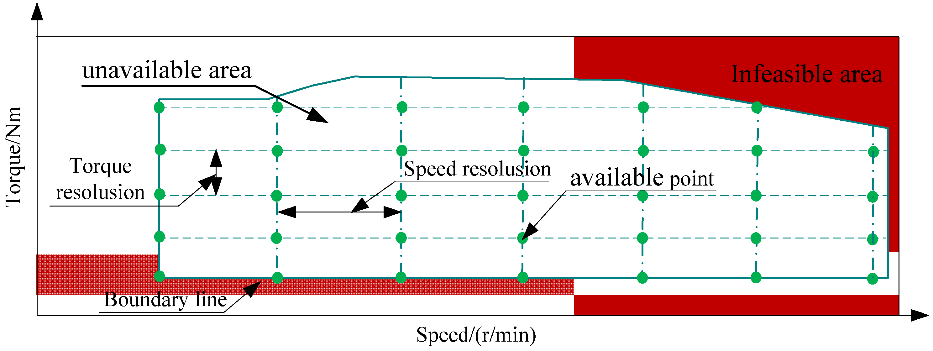
Another issue to consider is the valuation of the cost function for the infeasible states. An infinite cost is always used as the cost function for the state points in the infeasible area, which could result in the cost-to-go values, obtained by linear interpolation between an infinite cost-to-go and a finite one, for the feasible state points near the boundary line becoming infinite. Consequently, the actual infeasible domain is enlarged during the calculation process. Moreover, the control variables also need to be properly discretized. For the control variables, the proportion of the feasible region that can be utilized depends on its discretization resolution, as shown in Figure 2. Clearly, the number of available points increases as the discretization resolution increases. Additionally, the optimality of the DP-based control sequences improves, whereas the computation load is substantially increased.

Figure 2. Discretization of the control variables.

Figure 2. Discretization of the control variables.

In general, if the aforementioned problems are not fully taken into account and appropriately treated, then the relevant numerical errors would have a large impact on the final result. These issues for the case of PHEVs will be investigated in this paper.

The remainder of this paper is organized as follows: Section 2 provides an introduction and discusses systematic modeling for the targeted single-axis series-parallel plug-in hybrid electric bus (PHEB). The DP of the optimal control problem for the PHEB is formulated in Section 3. The numerical issues when solving the DP are investigated in Section 4. The results from the PHEB with two types of strategies are discussed in Section 5. Finally, conclusions are drawn in Section 6.

2. Plug-in Hybrid Powertrain Model

As an approach to solve global optimization problems over a finite horizon, DP is always used for solving the optimal energy management problem of HEVs [21,22,23]. In this paper, for the purpose of minimizing the fuel consumption of PHEVs over a given driving cycle, DP is responsible for finding the optimal power combination of the power components to meet the power demand of the vehicle, which is based on the vehicle dynamic model.

2.1. A Plug-in Hybrid Electric Bus Powertrain

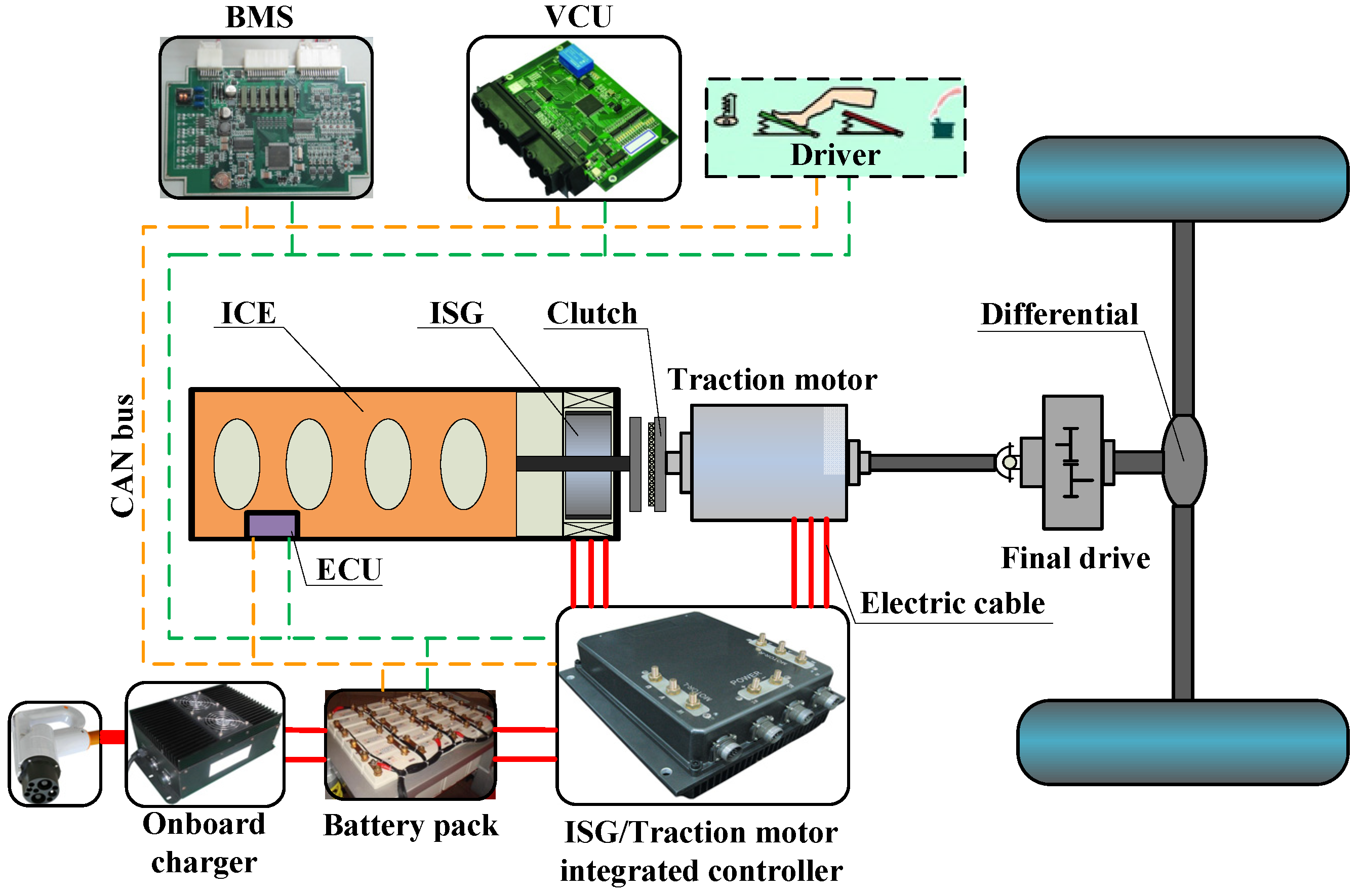
A single-axis series-parallel PHEB is taken as the research object, and its powertrain configuration is shown in Figure 3. It consists of a conventional internal combustion engine (ICE), an integrated starter and generator (ISG), a traction motor (TM), an automatically controllable friction clutch, a battery pack, an on-board battery charger and electronic control systems, which include a vehicle control unit (VCU), a battery management system (BMS), an integrated motor controller for the ISG and the TM, an ICE control unit, and so on. The technical parameters of the PHEB are summarized in Table 1.

Figure 3. Powertrain configuration of the series-parallel PHEB.

Figure 3. Powertrain configuration of the series-parallel PHEB.

Table 1. The PHEB main specifications.

Powertrain	Parameter	Value	Parameter	Value
ICE	Maximum power/kW	147	Maximum torque/Nm	730
ISG	Maximum power/kW	55	Maximum torque/Nm	500
TM	Maximum power/kW	166	Maximum torque/Nm	2080
Battery pack	Capacity/Ah	60	Voltage/V	576
Others	Curb weight/kg	12,500	Aerodynamic drag coefficient	0.55
	Gross weight/kg	18,000	Rolling resistance coefficient	0.0095
	Frontal area/m2	6.6	Transmission efficiency	0.93
	Tire rolling radius/mm	473	-	-

Table 1. The PHEB main specifications.

Powertrain	Parameter	Value	Parameter	Value
ICE	Maximum power/kW	147	Maximum torque/Nm	730
ISG	Maximum power/kW	55	Maximum torque/Nm	500
TM	Maximum power/kW	166	Maximum torque/Nm	2080
Battery pack	Capacity/Ah	60	Voltage/V	576
Others	Curb weight/kg	12,500	Aerodynamic drag coefficient	0.55
	Gross weight/kg	18,000	Rolling resistance coefficient	0.0095
	Frontal area/m2	6.6	Transmission efficiency	0.93
	Tire rolling radius/mm	473	-	-

For the PHEB powertrain, the ICE output is connected directly to the ISG rotor shaft and then connected to the clutch input plate. The TM rotor is connected directly to the clutch output plate. The power from the ICE, the ISG and the TM can be delivered directly to the rear drive wheels through the final drive and the differentials. The automatically controllable friction clutch is used to connect or disconnect the ICE/ISG torque with the TM torque. If the clutch input plate and output plate are connected, then the ICE/ISG torque can be delivered directly to the driving wheels, and the PHEB works in a parallel hybrid mode. When the clutch input plate and output plate are disconnected, the ICE/ISG can only output electricity, and the PHEB works in a series hybrid mode. Note that the ISG can instantaneously start the ICE once the ICE needs to work.

2.2. The Vehicle Model

The movement behavior of a vehicle along its moving direction is completely determined by all of the forces that act on it in the same direction. In the longitudinal direction, the major external forces acting on a two-axle vehicle include the rolling resistance of the front and rear tires, $F_f$; the aerodynamic drag, $F_w$; the climbing resistance, $F_i$; the acceleration resistance, $F_j$; and the tractive effort of the drive wheels, $F_d$. The dynamic equation for vehicle motion along the longitudinal direction is expressed by:

$$F_{\text{d}}=F_{\text{f}}+F_{\text{w}}+F_{\text{i}}+F_{\text{j}}=mgf\cdot \cos \alpha +\frac{1}{2}\cdot C_{\text{D}}\cdot A\rho \cdot v^2+mg\cdot \sin \alpha +\delta m\cdot \frac{\text{d}v}{\text{d}t}$$

(1)

where $m$ is the vehicle gross weight, $g$ is the acceleration due to gravity, $f$ is the rolling resistance coefficient, $\alpha$ is the road gradient, $C_{\text{D}}$ is the aerodynamic drag coefficient, $A$ is the vehicle frontal area, $\rho$ is the air density, $v$ is the vehicle velocity, $\delta$ is the mass factor that equivalently converts the rotational inertias of rotating components into translational mass, and $\frac{\text{d}v}{\text{d}t}$ is the vehicle acceleration.

The driving resistances depend on the current state of the vehicle and on the driver’s expectation at the next moment. During the simulation, the desired velocity at the next moment is determined from the driving cycle profile. Because the vehicle simulation system is a discrete-time system, the current acceleration, $a_k$, can be described as:

$$a_k=\frac{{v^{\prime }}_{k+1}-v_k}{t_{\text{step}}}$$

(2)

where $v_k$ is the current velocity, ${v^{\prime }}_{k+1}$ is the desired velocity at the next simulation step, and $t_{\text{step}}$ is the simulation time step.

By combining Equations (1) and (2), the vehicle torque requirements for the powertrain at the current step in the discrete-time space, $T_{\text{req}\_k}$, can be formulated as:

$$T_{\text{req}\_k}=\frac{r_{\text{d}}}{i_0{\eta }_{\text{T}}}\cdot (mgf\cdot \cos {\alpha }_k+\frac{1}{2}\cdot C_{\text{D}}\cdot A\rho \cdot v_k^2+mg\cdot \sin {\alpha }_k+\delta m\cdot a_k)$$

(3)

where $r_{\text{d}}$ is the dynamic radius of the wheel, $i_0$ is the ratio of the final gear, ${\eta }_{\text{T}}$ is the transmission efficiency, and ${\alpha }_k$ is the road gradient at the current step.

2.3. ICE Model

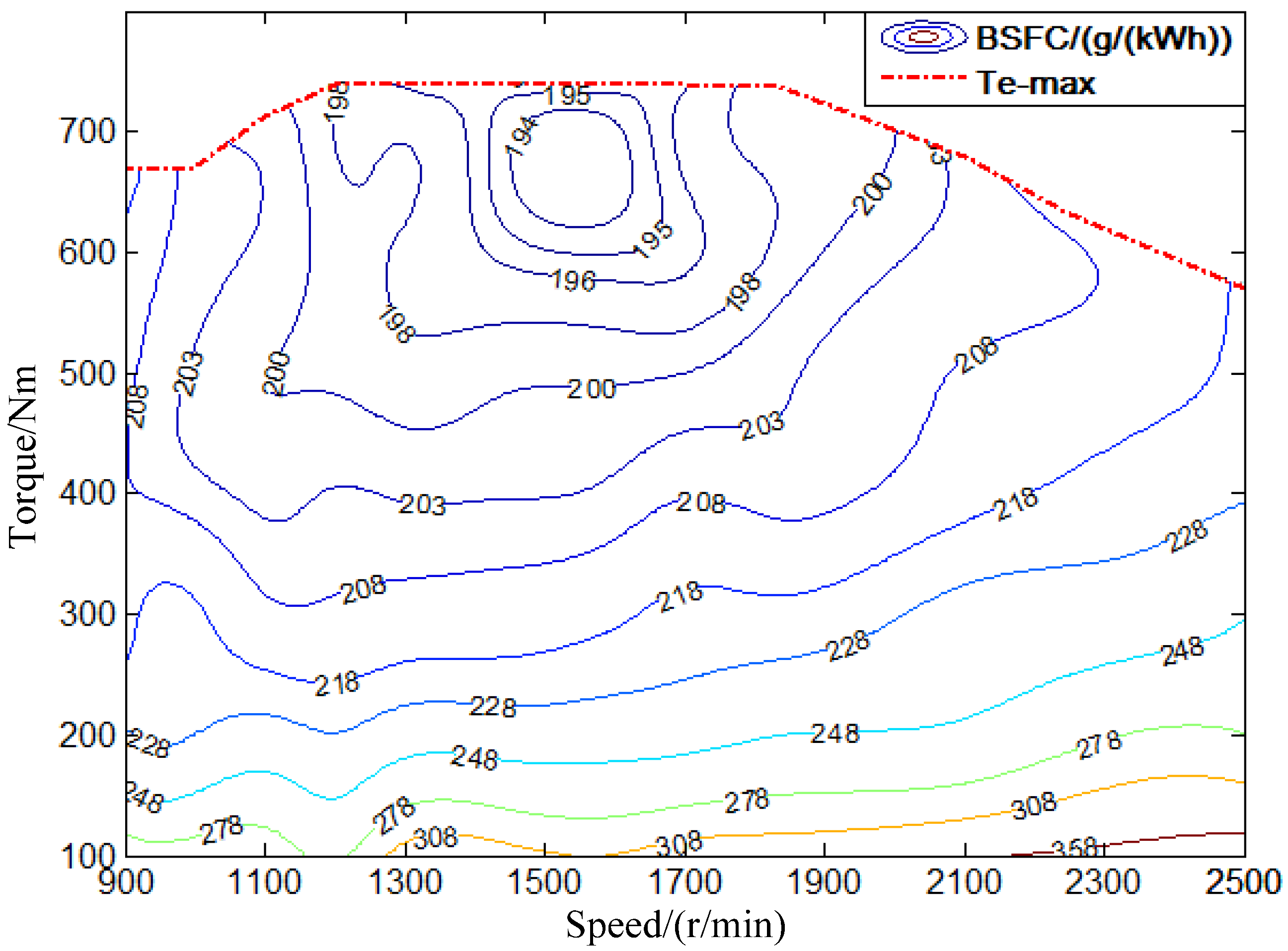
The experimental modeling method is used to develop the ICE model in the quasi-static vehicle model without considering its dynamic characteristics. The fuel consumption map of the ICE is expressed as the relationship between the crankshaft speed and the torque by a non-linear 3-D MAP from experimental ICE data. Figure 4 shows the fuel consumption map of a 6.5 L diesel engine. Note that BSFC is the abbreviation for brake specific fuel consumption.

Therefore, the ICE fuel consumption rate $g_{\text{e}}(n_{\text{e}},T_{\text{e}})$ at the operating point $(n_{\text{e}},T_{\text{e}})$, where the ICE outputs torque $T_{\text{e}}$ at speed $n_{\text{e}}$, is obtained from the following interpolation function:

$$g_{\text{e}}(n_{\text{e}},T_{\text{e}})=f(n_{\text{e}},T_{\text{e}})$$

(4)

In the discrete-time system, the ICE fuel consumption at the $k\text{th}$ simulation step, $V_{\text{fuel\_}k}$, is obtained by:

$$V_{\text{fuel\_}k}=\frac{1}{34380000\cdot {\rho }_{\text{fuel}}}\cdot n_{\text{e}\_k}\cdot T_{\text{e}\_k}\cdot g_{\text{e}}\left(n_{\text{e}\_k},T_{\text{e}\_k}\right)\cdot t_{\text{step}}$$

(5)

where ${\rho }_{\text{fuel}}$ is the fuel density and $n_{\text{e}\_k}$ and $T_{\text{e}\_k}$ are the speed and output torque of the ICE at the current step, respectively.

Figure 4. The ICE fuel consumption map.

Figure 4. The ICE fuel consumption map.

Then, the ICE fuel consumption $V_{\text{fuel}}$ during the simulation process is obtained by:

$$V_{\text{fuel}}={\displaystyle \sum _{k=1}^{L_{\text{sim}}}{V}_{\text{fuel\_}k}}$$

(6)

where $L_{\text{sim}}$ is the number of simulation steps, obtained as $L_{\text{sim}}=\frac{T_{\text{sim}}}{t_{\text{step}}}$, and $T_{\text{sim}}$ is the simulation period.

2.4. The ISG and TM Models

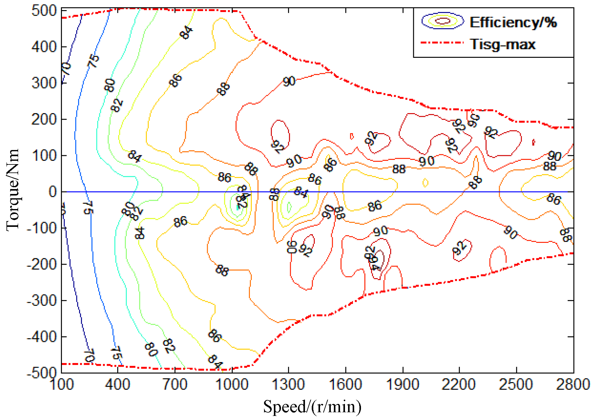
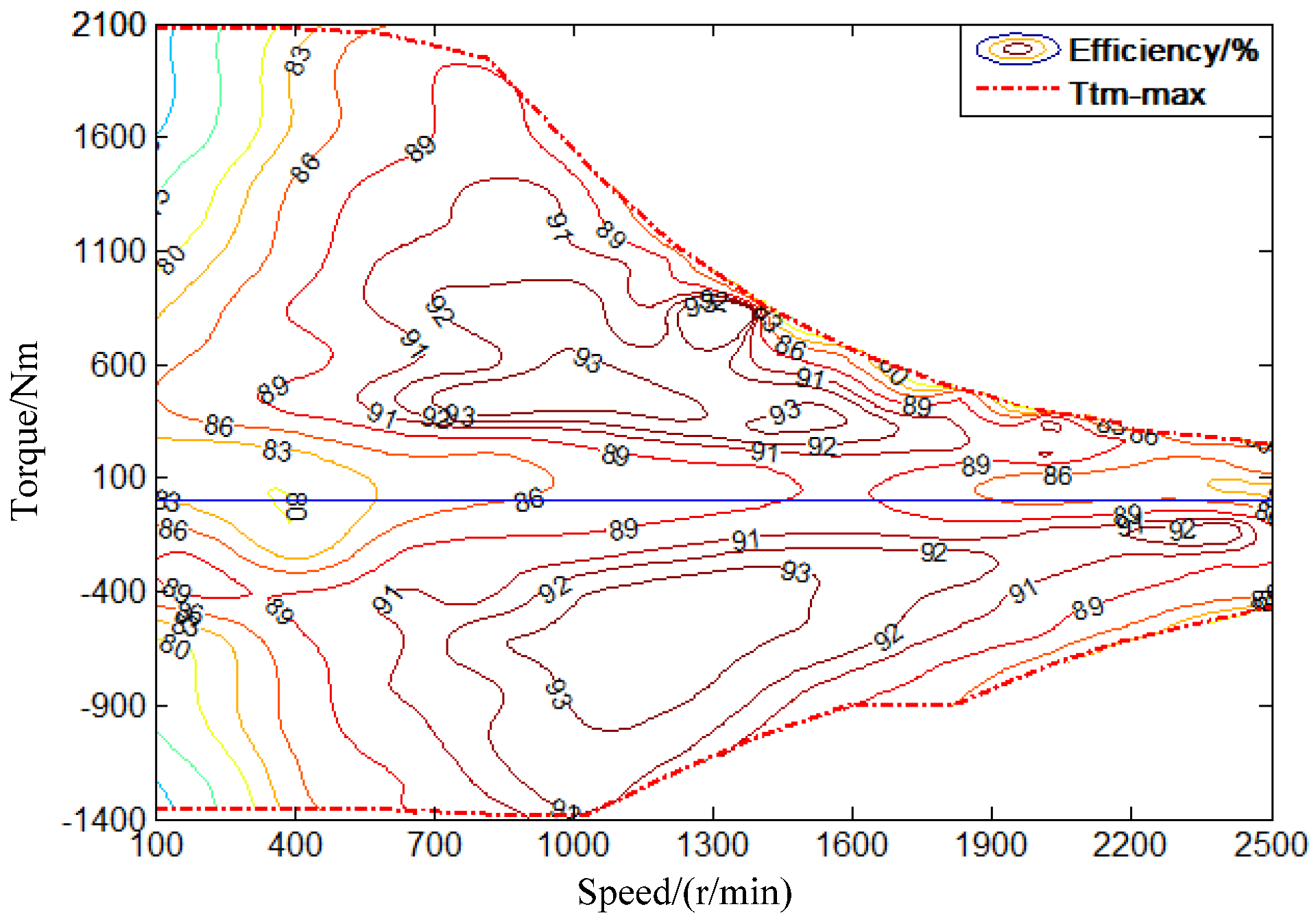
The experimental modeling method is also used to develop the ISG model and the TM model. Their efficiency characteristics are expressed as the relationship between the speed and the torque by a non-linear 3-D MAP from experimental data. Figure 5 shows the ISG efficiency map, and Figure 6 shows the TM efficiency map. The torque output model of the motor is similar to the ICE. The motor efficiency ${\eta }_{\text{m}}(n_{\text{m}},T_{\text{m}})$ at the operating point $(n_{\text{m}},T_{\text{m}})$ is obtained from the following interpolation function:

$${\eta }_{\text{m}}(n_{\text{m}},T_{\text{m}})=f(n_{\text{m}},T_{\text{m}})$$

(7)

where $n_{\text{m}}$ is the speed of the motor and $T_{\text{m}}$ is the motor output torque, which is defined as positive during propelling and negative during regenerative braking.

Figure 5. The ISG efficiency map.

Figure 5. The ISG efficiency map.

Figure 6. The traction motor efficiency map.

Figure 6. The traction motor efficiency map.

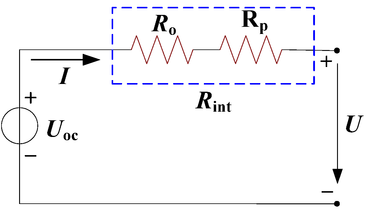
2.5. The Battery Model

A lithium-ion battery is used, which can be modeled with a static equivalent circuit [24]. In this paper, the Rint model, which is based on experimental data of battery charging-discharging, is used due to its simplicity and effectiveness for lithium-ion batteries. This model is illustrated in Figure 7.

Figure 7. The Rint battery model.

Figure 7. The Rint battery model.

Here $U_{\text{oc}}$ is the battery open-circuit voltage, which is related to the SoC and the battery temperature $T_{\text{b}}$ and can be obtained from the interpolation function $U_{\text{oc}}=f(SoC,T_{\text{b}})$ based on the experimental data; $I$ is the battery charging-discharging current, which is defined as positive during discharging and negative during charging; $R_{\text{int}}$ is the battery internal resistance, including an Ohmic resistance $R_{\text{o}}$ and a polarization resistance $R_{\text{p}}$, which can be obtained from the interpolation function $R_{\text{int}}=f(SoC,T_{\text{b}},I)$; and $U$ is the load voltage of the battery, which can be obtained by $U=U_{\text{oc}}-I\cdot R_{\text{int}}$.

Based on the equivalent circuit shown in Figure 7, the following equations can be obtained:

$$P_{\text{bat}}=U\cdot I=(U_{\text{oc}}-I\cdot R_{\text{int}})\cdot I=U_{\text{oc}}\cdot I-I^2\cdot R_{\text{int}}$$

(8)

where $P_{\text{bat}}$ is the electric power provided by the battery, which is positive during discharging and negative during charging.

In addition, $P_{\text{bat}}$ is determined by the ISG and the TM as shown in the following equation:

$$P_{\text{bat}}={\left(\begin{array}{c}\mathrm{sgn}(T_{\text{ISG}})\cdot T_{\text{ISG}}\cdot n_{\text{ISG}}\\ \mathrm{sgn}(T_{\text{TM}})\cdot T_{\text{TM}}\cdot n_{\text{TM}}\end{array}\right)}^{\text{T}}\left(\begin{array}{c}{\eta }_{\text{TM}}^{-\mathrm{sgn}(T_{\text{TM}})}\\ {\eta }_{\text{ISG}}^{-\mathrm{sgn}(T_{\text{ISG}})}\end{array}\right)$$

(9)

where $T_{\text{ISG}}$, $n_{\text{ISG}}$ and ${\eta }_{\text{ISG}}$ are the output torque, speed and working efficiency of the ISG, respectively, and $T_{\text{TM}}$, $n_{\text{TM}}$ and ${\eta }_{\text{TM}}$ are the output torque, speed and working efficiency of the TM, respectively.

Equation (8) is transformed to the following form:

$$I=\frac{U_{\text{oc}}-\sqrt{U_{\text{oc}}^2-4R_{\text{int}}\cdot P_{\text{bat}}}}{2R_{\text{int}}}$$

(10)

The first-order derivative of the battery SoC with respect to time can be expressed as follows:

$$\frac{\text{d}SoC}{\text{d}t}=-\frac{I}{C}=-\frac{U_{\text{oc}}-\sqrt{U_{\text{oc}}^2-4R_{\text{int}}\cdot P_{\text{bat}}}}{2R_{\text{int}}\cdot C}$$

(11)

where C is the nominal capacity of the battery.

Equation (11) is transformed to a discrete form, as follows:

$$So{C}_{k+1}=So{C}_k-\frac{U_{\text{oc}\_k}-\sqrt{U_{\text{oc}\_k}^2-4R_{\mathrm{int}\_k}\cdot P_{\text{bat}\_k}}}{2R_{\mathrm{int}\_k}\cdot C}$$

(12)

where $So{C}_{k+1}$ is the battery SoC at the (k+1)th step and $So{C}_k$, $U_{\text{oc}\_k}$, $P_{\text{bat}\_k}$ and $R_{\mathrm{int}\_k}$ are the SoC, open-circuit voltage, electric power and internal resistance of the battery at the kth step, respectively.

The electricity consumption Q during the simulation process is obtained by:

$$Q=\frac{1}{3600}\cdot {\displaystyle \sum _{k=1}^{L_{\text{sim}}}{U}_{\text{oc}\_k}\cdot I_k\cdot t_{\text{step}}}$$

(13)

where $I_k$ is the battery charging-discharging current at the kth step.

3. Dynamic Programming

3.1. Formulating Dynamic Programming

Prior to formulating the DP, the control variables and state variables need to be determined. In this paper, the state variables, such as the vehicle speed $v$ and SoC, reflect the state of the PHEB. Because DP is implemented over the known driving cycle, the vehicle speed at every stage is known. Therefore, SoC is chosen as the only state variable in this work. There are many control variables in the PHEB, such as the ICE output torque $T_{\text{e}}$, ICE output speed $n_{\text{e}}$, TM output torque $T_{\text{TM}}$, TM output speed $n_{\text{TM}}$, ISG output torque $T_{\text{ISG}}$, ISG output speed $n_{\text{ISG}}$, and hydraulic brake torque $T_{\text{b}}$. However, only two control variables, $T_{\text{e}}$ and $T_{\text{TM}}$, are independent, and these two variables are chosen as the independent control variables in this work.

In the discrete-time format, the PHEB system can be expressed as follows:

$$x_{k+1}=f(x_k,u_k)$$

(14)

where $x_k$ and $u_k$ are the state variable and the control variable, respectively.

Compared with HEVs, whose battery acts as a power equalizer to improve the ICE operating efficiency with the expectation of the same SoC at the start and end of a trip, PHEVs have a larger battery and can replace a certain amount of fossil energy with grid electricity. In general, the exhaust emissions from the hybrid electric bus are not taken into consideration. In studying the object PHEB in this paper, we only focus on minimizing the fuel consumption. Then, the optimal control problem is to find the control sequences to minimize the following cost function:

$$J={\displaystyle \sum _{k=0}^{N-1}L\left(x_k,u_k\right)}$$

(15)

where N is the stage number of the driving cycle and L is the instantaneous cost.

To ensure safe/smooth operation of the components, such as the ICE, ISG, TM and battery, during the solving process, it is necessary to satisfy constraints related to their ratings and the power flow between them. The physical constraints on the states and the inputs are denoted by the following inequalities and equalities:

$$\{\begin{array}{l}SO{C}_{\min }\le SO{C}_k\le SO{C}_{\max }\\ n_{\text{e\_min}}\le n_{\text{e}\_k}\le n_{\text{e\_max}}\\ T_{\text{e\_min}}\left(n_{\text{e\_}k}\right)\le T_{\text{e}\_k}\le T_{\text{e\_max}}\left(n_{\text{e\_}k}\right)\\ n_{\text{ISG\_min}}\le n_{\text{ISG}\_k}\le n_{\text{ISG\_max}}\\ T_{\text{ISG\_min}}\left(n_{\text{ISG\_}k},SO{C}_k\right)\le T_{\text{ISG\_}k}\le T_{\text{ISG\_max}}\left(n_{\text{ISG\_}k},SO{C}_k\right)\\ n_{\text{TM\_min}}\le n_{\text{TM}\_k}\le n_{\text{TM\_max}}\\ T_{\text{TM\_min}}\left(n_{\text{TM}\_k},SO{C}_k\right)\le T_{\text{TM\_}k}\le T_{\text{TM\_max}}\left(n_{\text{TM}\_k},SO{C}_k\right)\\ T_{\text{req\_}k}\text{=}{T}_{\text{e}\_k}\text{+}{T}_{\text{ISG\_}k}\text{+}{T}_{\text{TM\_}k}\text{+}{T}_{\text{b\_}k}/i_0\end{array}$$

(16)

where $n_{\text{ISG\_}k}$ and $T_{\text{ISG\_}k}$ are the speed and output torque of the ISG at the kth step, respectively; $n_{\text{TM}\_k}$ and $T_{\text{TM\_}k}$ are the speed and output torque of the TM at the kth step, respectively; $T_{\text{b\_}k}$ is the hydraulic brake torque at the kth step; and the subscripts min and max in the variables denote the maximum and minimum of those variables, respectively.

3.2. Implementing Dynamic Programming

During the backward simulation procedure, the DP problem can be described by the recursive Equations (17) and (18). The sub-problem for the (N – 1)th step is:

$$J_{N-1}^{*}(x_{N-1})=\underset{u_{N-1}}{\min }\left[L(x_{N-1},u_{N-1})\right]$$

(17)

For the $k\text{th}$ ($0\le k<N-1$) step, the sub-problem is:

$$J_k^{*}(x_k)=\underset{u_k}{\min }\left[L(x_k,u_k)+J_{k+1}^{*}(x_{k+1})\right]$$

(18)

where $J_k^{*}(x_k)$ is the optimal cost-to-go function at state $x_k$ from the kth simulation step to the terminal of the driving cycle and $x_{k+1}$ is the state in the $(k+1)\text{th}$ stage when the control variable $u_k$ is applied to state $x_k$ at the $k\text{th}$ stage according to Equation (14).

Before recursive Equations (17) and (18) are solved in reverse, it is necessary for the continuous variables to be discretized. The continuous state SoC is discretized into finite points, and the number of discretized state, S, is:

$$S=\raisebox{1ex}{$\left(So{C}_{\max }-So{C}_{\min }\right)$}\!\left/ \!\raisebox{-1ex}{$\mathrm{\Delta }SoC$}\right.$$

(19)

where $\mathrm{\Delta }SoC$ is the increment of the discretized SoC and $So{C}_{\max }$ and $So{C}_{\min }$ are the upper and lower constrains of SoC, respectively.

In addition, the independent control variables, $T_{\text{e}}$ and $T_{\text{m}}$, are all continuous and also need to be discretized into finite points. Due to the coupling relationship between the torque variables, $T_{\text{e}}$ and $T_{\text{m}}$ have the same discretization resolution, denoted by $\mathrm{\Delta }T$, which is defined here as the torque increment.

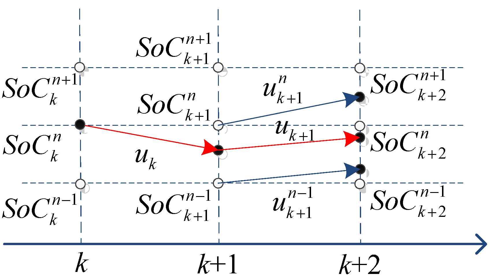
During the backward simulation procedure, the model output $So{C}_{k+1}$ of the system state SoC based on Equation (12) is continuous in the state space, and it does not generally coincide with the nodes of the state grid but is rather between them, as depicted in Figure 8. When evaluating the function $J_k^{*}(x_k)$ at every grid point, such as $So{C}_k^{n-1}$, $So{C}_k^n$, $So{C}_k^{n+1}$, and so on, $J_{k+1}^{*}(x_{k+1})$ is evaluated by interpolation if the model output $So{C}_{k+1}$ does not fall exactly on grid points.

Figure 8. The interpolation diagram during the backward simulation.

Figure 8. The interpolation diagram during the backward simulation.

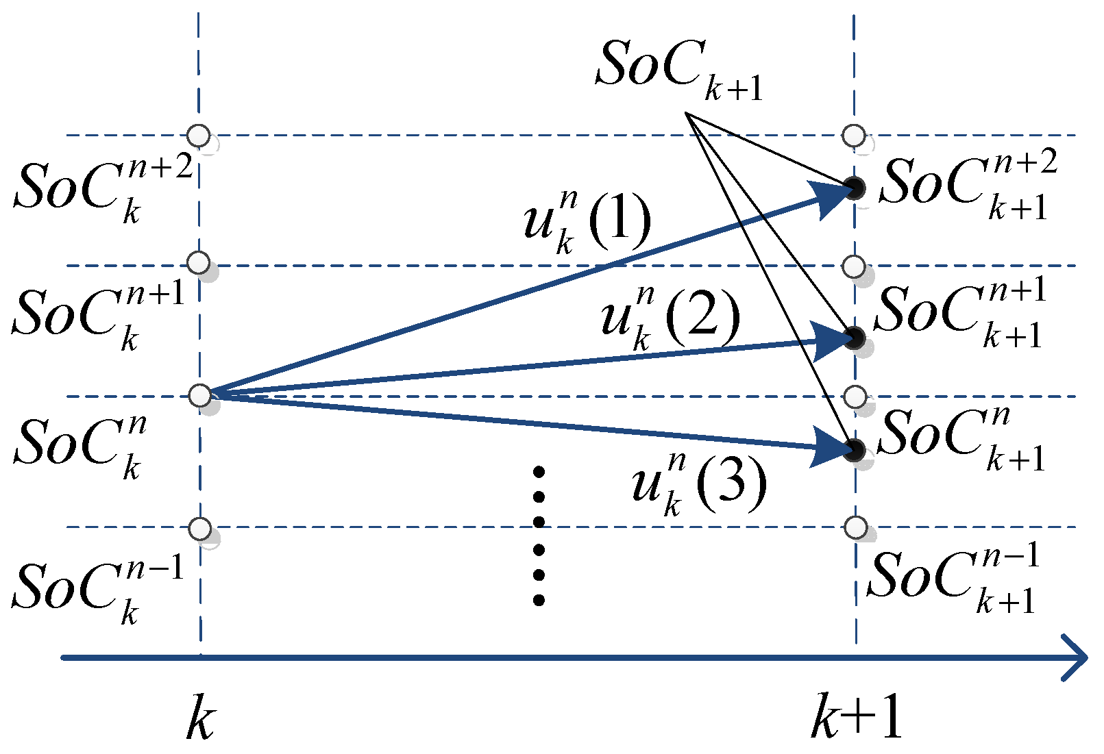
During the backward simulation, the optimal controls at every grid point are obtained. When the initial SoC is specified, the optimal control sequences can be found through a forward simulation. During the forward simulation procedure, the interpolation is also needed to find the optimal control sequences, as shown in Figure 9. When the optimal control at the kth stage is $u_k$, the optimal control $u_{k+1}$ at the $k+1\text{th}$ stage is obtained through interpolation between $u_{k+1}^{n-1}$ and $u_{k+1}^n$, which are the optimal controls at the grid points $So{C}_{k+1}^{n-1}$ and $So{C}_{k+1}^n$, respectively, at the $k+1\text{th}$ stage.

Figure 9. The interpolation diagram during the forward simulation.

Figure 9. The interpolation diagram during the forward simulation.

4. Numerical Issues of the DP

The errors that occur during implementation of the DP procedure result from approximating the valuation when the actual state does not coincide with the nodes of the state grid, as in Figure 8 and Figure 9. Additionally, these errors are closely related to the discretization resolution of relevant continuous variables. In this section, the interaction mechanism between the accuracy of the calculated results and the numerical issues, such as the resolution issue of the discretized variables and the boundary issue, is investigated with consideration of the computational load.

4.1. Resolution Study

For the vehicles, because of the correlation between the sampling period of the given driving cycle and the total vehicle energy demand under this driving cycle, the stage step, the discretization step of the time space, is chosen to equal to the sampling period such that the stage number N is equal to the number of sampling points of the driving cycle. Thus, the discretization resolution of the state space and the control variables is investigated in the following section.

4.1.1. Resolution of the State Variable

The increment of the discretized state variable SoC, $\mathrm{\Delta }SoC$, represents its resolution. The dynamics of the battery SoC is inherently determined by the sampling period, the battery capacity and the charging/discharging current, which is dependent on the output power of the motor. However, the only adjustable variable relative to the SoC dynamics is the torque increment $\mathrm{\Delta }T$ in this work. 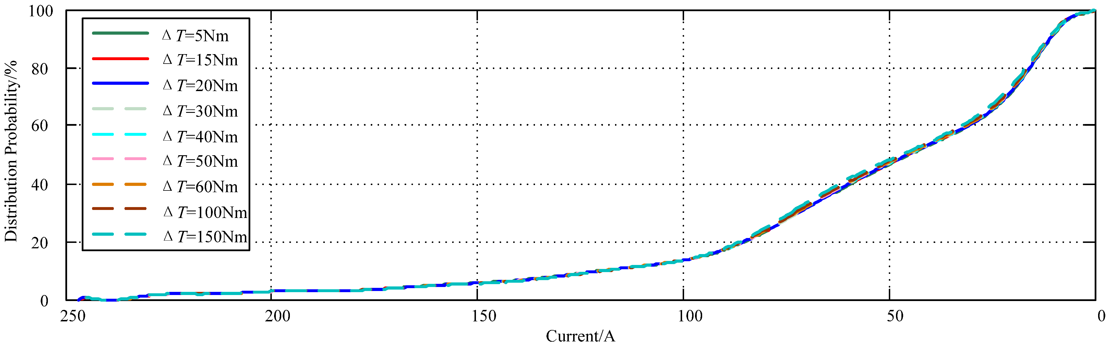Moreover, it is clear that the smaller $\mathrm{\Delta }T$ is, the more accurate are the results calculated by DP. The relationship between the battery charging/discharging current and the different $\mathrm{\Delta }T$ is investigated, and the results are presented in Figure 10.

As shown in Figure 10, within certain limits, the increase in $\mathrm{\Delta }T$ does not clearly influence the battery working current and the computational load is noticeably reduced. Based on the mathematical principle of DP, the discretization resolution of the state space and the discretization resolution of the control variables are independent of the calculated results. Therefore, during the procedure for investigating the SoC discretization resolution, the difference in the $\mathrm{\Delta }T$ does not influence the rate of convergence of the calculated results.

Figure 10. The distribution probability of the absolute value of the battery charging/discharging current for different $\mathrm{\Delta }T$.

Figure 10. The distribution probability of the absolute value of the battery charging/discharging current for different $\mathrm{\Delta }T$.

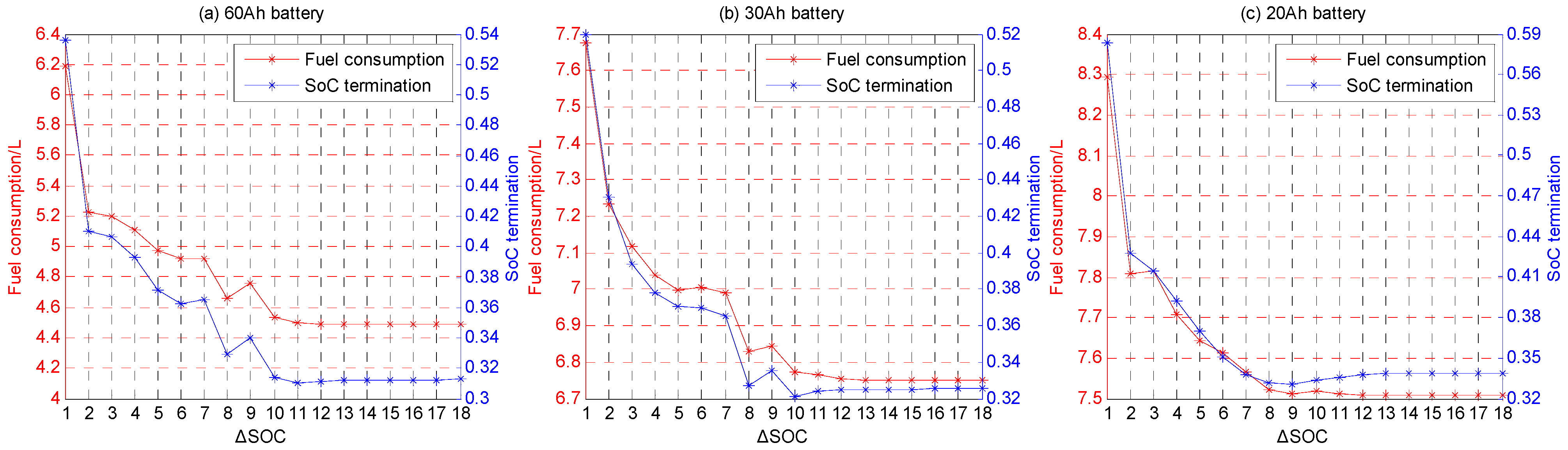
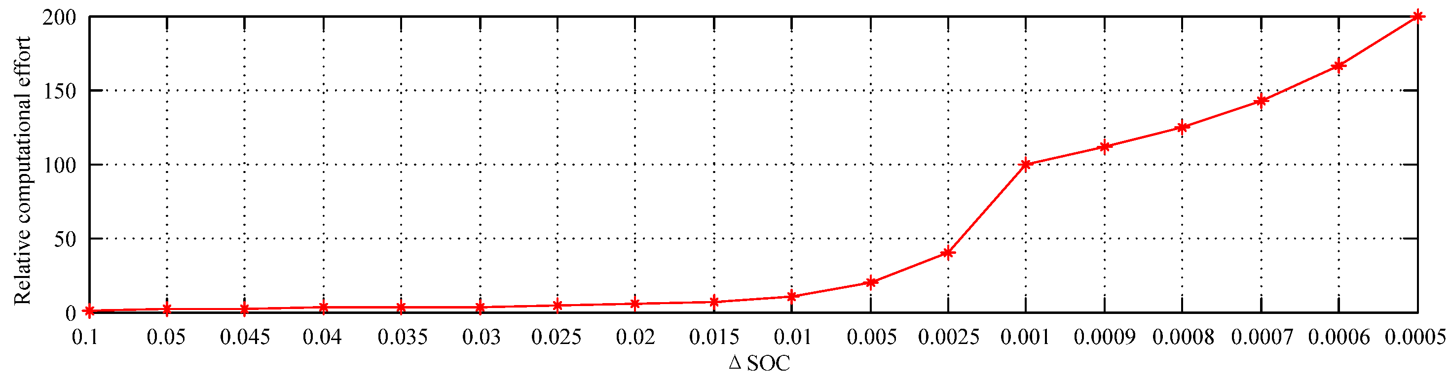
Here, $\mathrm{\Delta }T$ is chosen as 30 Nm, and the relationship between $\mathrm{\Delta }SoC$ and the calculated results for batteries with different capacities is shown in Figure 11. The computational load with different $\mathrm{\Delta }SoC$ is also checked, and the results are shown in Figure 12. Note that the abscissa values of the three graphs in Figure 11 are consistent with those in Figure 12.

Figure 11. The results calculated by DP with different $\mathrm{\Delta }SoC$.

Figure 11. The results calculated by DP with different $\mathrm{\Delta }SoC$.

Figure 12. The relative computational load for different $\mathrm{\Delta }SoC$.

Figure 12. The relative computational load for different $\mathrm{\Delta }SoC$.

From Figure 11 and Figure 12, it is clear that the fuel consumption decreases as $\mathrm{\Delta }SoC$ decreases and tends to be stable after $\mathrm{\Delta }SoC$ is sufficiently small; the SoC termination follows the same trend. Unfortunately, the computational load increases many fold when $\mathrm{\Delta }SoC$ decreases. In addition, the convergence rate of the calculated results is closely related to the battery capacity, and the slower the convergence speed is, the larger the battery capacity will be. In other words, the maximum $\mathrm{\Delta }SoC$ through which the accuracy could be ensured increases as the battery capacity decreases. Thus, the appropriate $\mathrm{\Delta }SoC$, which requires a minimum computational load to ensure accuracy, can be obtained according to the battery capacity.

4.1.2. Resolution of the Control Variables

As mentioned above, the torque increment $\mathrm{\Delta }T$ represents the resolution of the control variables. When a lower discretization resolution is chosen, the feasible region of the power components is not effectively utilized and the optimality of the calculated results is inherently degraded. However, a higher discretization resolution corresponds to a higher computational load. Due to the decoupling characteristics between the discretization resolution of the state space and the discretization resolution of the control variables mentioned above, $\mathrm{\Delta }SoC$ is set constant at 0.001 when investigating the influence of $\mathrm{\Delta }T$ on the calculated results. The calculated results are shown in Figure 13, and the corresponding computational load is shown in Figure 14.

Figure 13. The results calculated by DP with different $\mathrm{\Delta }T$.

Figure 13. The results calculated by DP with different $\mathrm{\Delta }T$.

Figure 14. The relative computational load for different $\mathrm{\Delta }SoC$.

Figure 14. The relative computational load for different $\mathrm{\Delta }SoC$.

As shown in Figure 13, the SoC termination is almost not influenced by $\mathrm{\Delta }T$, and the fuel consumption gradually tends to the optimal value with decreasing $\mathrm{\Delta }T$. For HEVs and PHEVs, the fuel consumption is generally the optimization goal, and ICE is the only component that consumes fuel. The specific fuel consumption of ICE is related to its capacity, calibrating conditions and so on; thus, the fuel consumption map of ICE needs to be taken into consideration when selecting $\mathrm{\Delta }T$.

Compared with $\mathrm{\Delta }SoC$, the influence of $\mathrm{\Delta }T$ on the computational load is very mild, as shown in Figure 14. When the maximum $\mathrm{\Delta }T$ is 400 times greater than the minimum, the difference between the corresponding computational loads is less than 4-fold. This result is the reason why the discretization of control variables is not necessary to be implemented in every computation when solving DP. Therefore, the extent to which $\mathrm{\Delta }T$ impacts the computational load is dependent on the frequency that discretization is implemented during the calculation.

4.2. Boundary Issue

When implementing DP, the boundary issue can be divided into two parts: the boundary issue of the state space and the boundary issue of the feasible region of control variables. In contrast to the optimal control problem of HEVs, whose state variable SoC remains constant within the preset range, the SoC trajectory of PHEVs monotonically decreases overall, as shown in Figure 15. Correspondingly, the boundary issue of the state space influencing the DP results exists throughout the solving procedure of DP for HEVs’ optimal control problem, whereas it only exists near the start and end of the trip for PHEVs. Therefore, it could be negligible to the accuracy of the results calculated by DP when using DP to solve the optimal control problem for PHEVs.

Figure 15. The optimal SoC trajectory of HEVs and PHEVs.

Figure 15. The optimal SoC trajectory of HEVs and PHEVs.

The boundary issue of the feasible region of control variables is that the available control points on the boundary lines face the risk of being missed, which is essentially derived from the discretization of the control variables. It has been actually embodied in the influence of the discretization resolution on the results calculated by DP.

In summary, from the results presented in Figure 11 and Figure 13, it could be observed that the convergence characteristics of the SoC termination are related to $\mathrm{\Delta }SoC$ but not influenced by $\mathrm{\Delta }T$. Thus, for the optimal control problem of PHEVs, the SoC trajectory is determined by the discretization resolution of the state variable SoC, whereas the optimality of the fuel consumption is primarily dependent on the discretization resolution of the state variable SoC and the discretization resolution of the control variables.

5. Application Example

In previous works [24], we defined the basic PHEV operating modes as pure electric driving (PED), hybrid driving charge depleting (HDCD) and hybrid driving charge sustaining (HDCS) based on the battery SoC profile and developed the PED + HDCD + HDCS strategy, which is an optimal online strategy that is practical for PHEVs. This strategy is optimally composed of the PED mode, the HDCD mode and the HDCS mode. In this section, DP is utilized to solve the optimal control problem of the PHEB presented in Section 2. The results obtained by DP are compared with the simulation results of the PHEB with the PED + HDCD + HDCS strategy.

The Chinese Standard Urban Driving Cycle (CSUDC), which is shown in Figure 16, is selected to be used during the simulation experiment. The trip distance is 180 km, which is attained by successively repeating the same driving cycle 31 times. Additionally, the vehicle is loaded with 65% of a full load.

Figure 16. Velocity profile of the CSUDC cycle.

Figure 16. Velocity profile of the CSUDC cycle.

Prior to conducting the simulation experiments, it is assumed that the battery of the PHEB has been fully charged from the power grid. Note that the PHEB is not allowed to implement regenerative braking when the battery SoC is higher than 80% for the purpose of protecting the battery. When implementing the DP, the $\mathrm{\Delta }SoC$ and the $\mathrm{\Delta }T$ are set to 0.5% and 5 Nm, respectively. 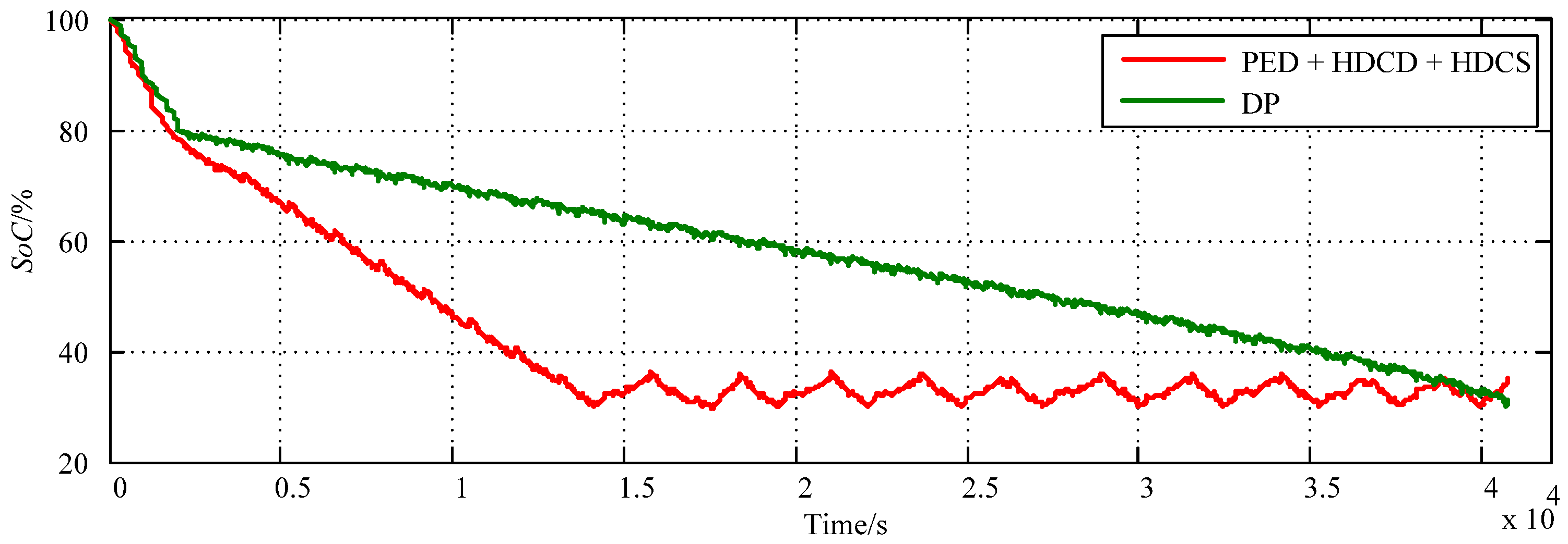The SoC trajectories of the PHEB with two types of control strategies are shown in Figure 17.

Figure 17. The SoC trajectories under two types of strategies.

Figure 17. The SoC trajectories under two types of strategies.

When the battery SoC is higher than 80%, the trends of the two SoC trajectories are similar, and the slight difference between them results from the ICE often being turned on to propel the vehicle under the DP-based strategy whereas the ICE is turned off for the PED + HDCD + HDCS strategy. When the battery SoC is between 80% and 30%, the battery SoC acquired by DP linearly decreases overall. Moreover, the available energy from the battery is exhausted only at the end of the trip, which provides the best benchmark for improving the online strategy. 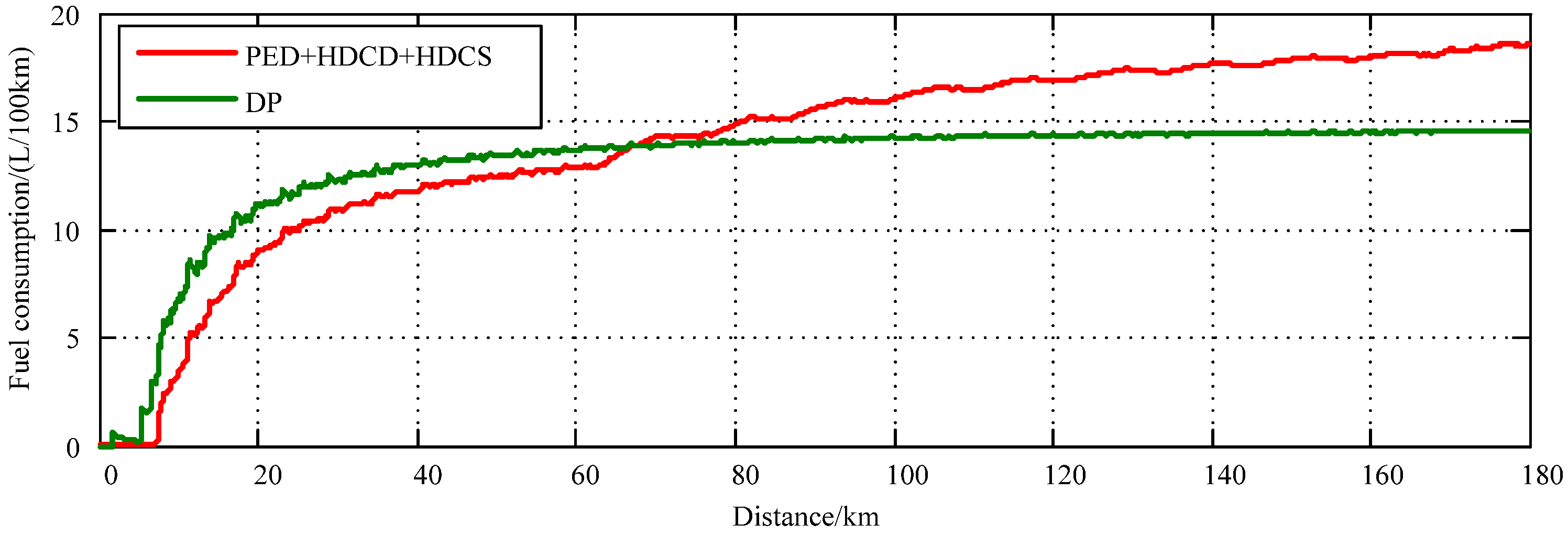Figure 18 shows the relationship between the trip distance and the fuel consumption per 100 km of the PHEB with the two types of strategies.

Figure 18. The relationship curve between fuel economy and trip distance under the two types of strategies.

Figure 18. The relationship curve between fuel economy and trip distance under the two types of strategies.

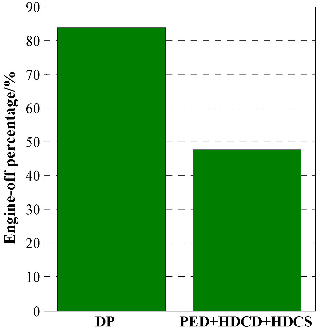
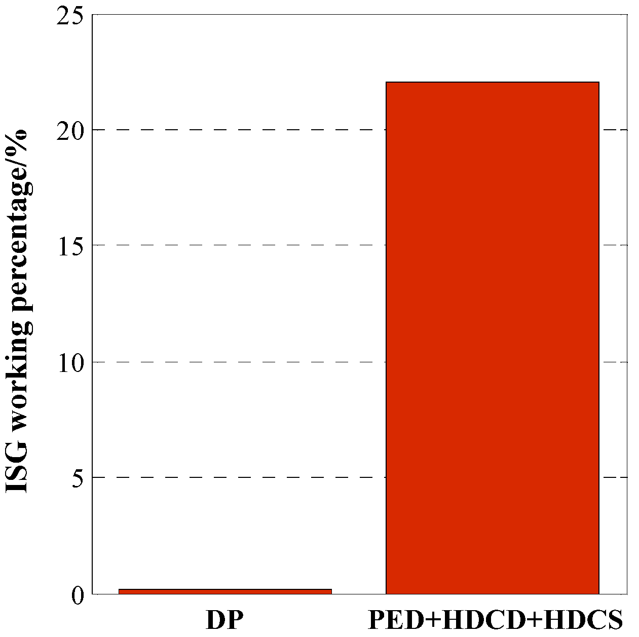
The fuel economy of the PHEB with the PED + HDCD + HDCS strategy is better than the results calculated by DP in the first fraction of the trip, as shown in Figure 18. However, the latter gradually becomes superior to the former as the trip distance increases. The reason for this result is that the DP-based strategy can coordinate different components of the PHEB powertrain to efficiently work from a global perspective. The shutdown proportion of the ICE and the ISG, which is performed by DP, is higher than that under the PED + HDCD + HDCS strategy, as shown in Figure 19 and Figure 20, respectively. Moreover, the ICE under the DP-based strategy works in the higher efficiency area, as shown in Figure 21 and Figure 22.

Figure 19. The ICE shutdown percentage under the two types of strategies.

Figure 19. The ICE shutdown percentage under the two types of strategies.

Figure 20. The ISG working percentage under the two types of strategies.

Figure 20. The ISG working percentage under the two types of strategies.

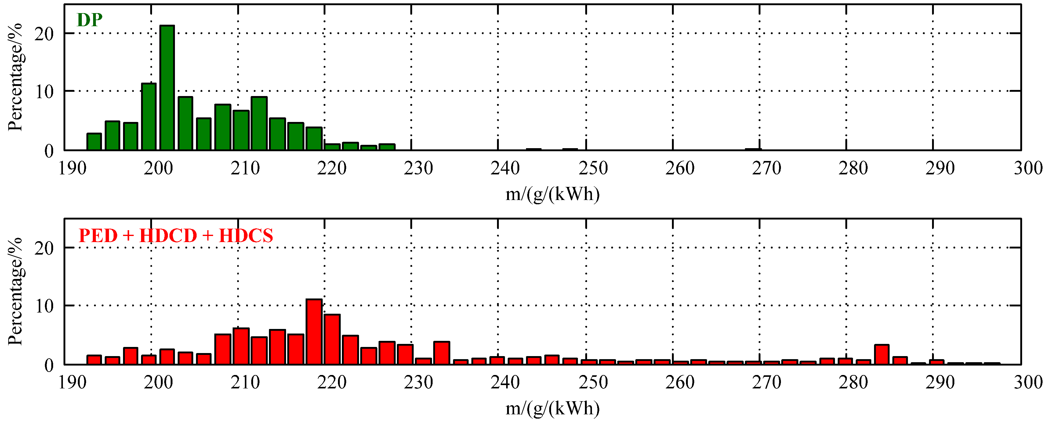
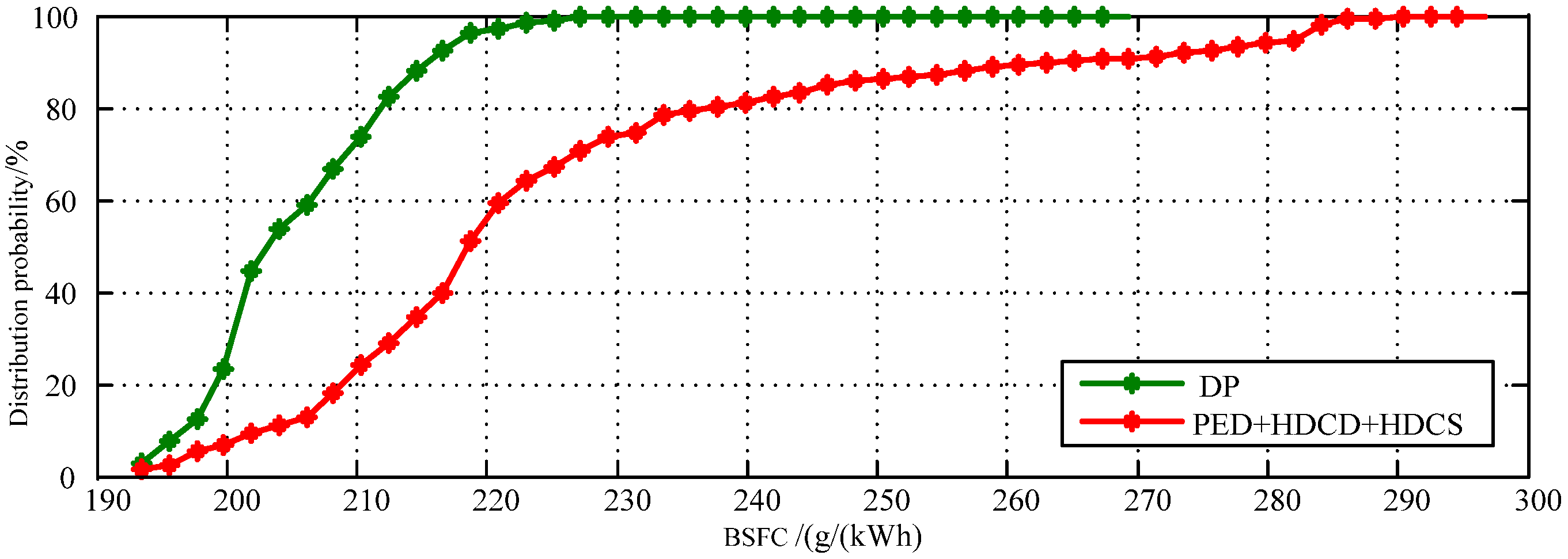
From the results presented in Figure 21, it is clear that the proportion of the ICE working points calculated by DP in the higher efficiency area is clearly greater than that under the PED + HDCD + HDCS strategy. Consequently, the distribution probability of the BSFC of the ICE working points in the results calculated by DP is considerably better than that under the PED + HDCD + HDCS strategy, as shown in Figure 22.

Figure 21. The statistical results of the BSFC of the working points of the ICE under the two types of strategies.

Figure 21. The statistical results of the BSFC of the working points of the ICE under the two types of strategies.

Figure 22. The distribution probability of the BSFC of the working points of the ICE under the two types of strategies.

Figure 22. The distribution probability of the BSFC of the working points of the ICE under the two types of strategies.

From the comparative analysis mentioned above, the drawback of the online strategy is clear. Then, the goal and the effective plan to improve the online strategy could be easily drawn.

6. Conclusions

We constructed a DP-based optimal control algorithm for a PHEB and investigated the interaction mechanism between the accuracy of the calculated results and the numerical issues, such as the resolution issue of the discretized variables and the boundary issue with consideration of the computational load. The main conclusions are as follows:

(1)

Numerical issues emerged when the optimal control problem of PHEVs was solved using DP. A single-axis series-parallel PHEB was modeled, and its systematic model was constructed for studying these issues. Then, the discretization resolution of the relevant variables and the boundary issue of their feasible region were investigated.

(2)

The battery SoC trajectory is determined by the discretization resolution of the state variable SoC, whereas the optimality of the fuel consumption is primarily dependent on the discretization resolution of the state variable SoC and the discretization resolution of the control variables. Additionally, the lowest discretization resolution of the state variable SoC with maintained accuracy is closely related to the battery capacity, whereas the fuel consumption map of ICE needs to be taken into consideration when selecting the discretization resolution of the control variables.

(3)

The computational load increases many fold as the discretization resolution of the state variable SoC increases. However, the influence of the discretization resolution of the control variables on the computational load is very mild. Moreover, the extent to which it impacts the computational load depends on the frequency with which the discretization is implemented during the calculation.

(4)

A simulation experiment was performed, and the results from two types of strategies were compared. The DP-optimized result provided the maximum potentiality of an energy management strategy for PHEVs, which serves an optimized target for other online control strategies by proper calibration methods.