
Acceleration Slip Regulation Strategy for Distributed Drive Electric Vehicles with Independent Front Axle Drive Motors

Abstract
:1. Introduction
2. System Model


| Parameter | Value |
|---|---|
| Vehicle mass | 1,500 kg |
| Driving axle | front |
| Number of motors | 2 |
| Motor Power | 20 kW |
| Maximum speed | 8,000 r/min |
| Gear ratio | 7.8 |
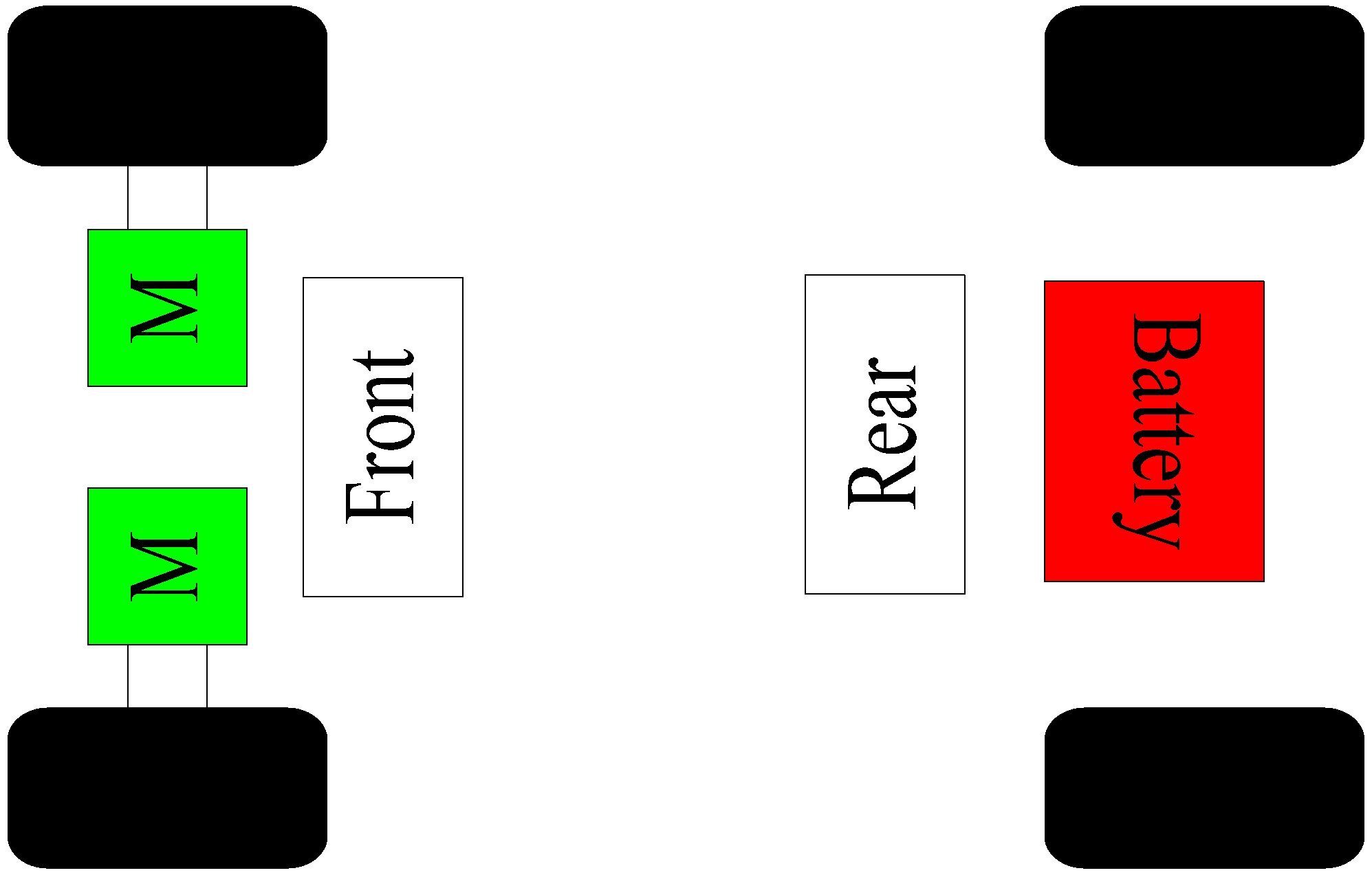
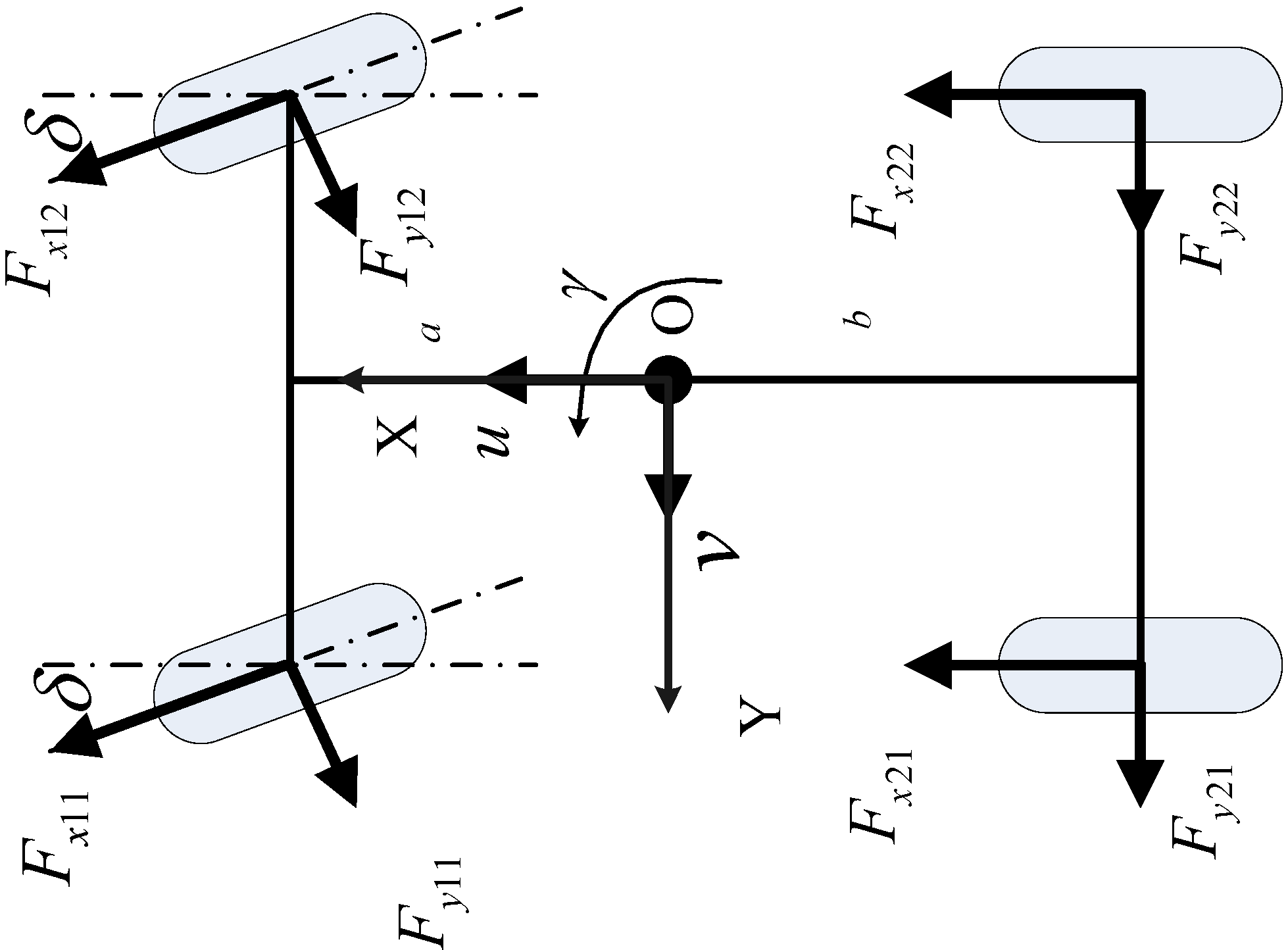
2.1. Vehicle Dynamic Model

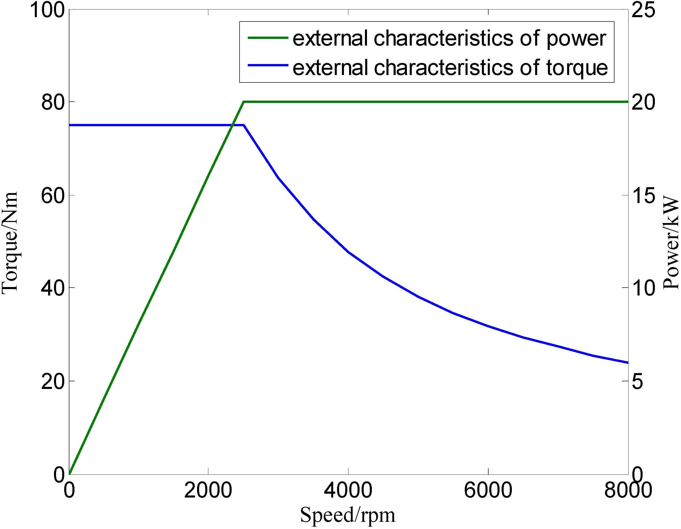
2.2. Motor Model

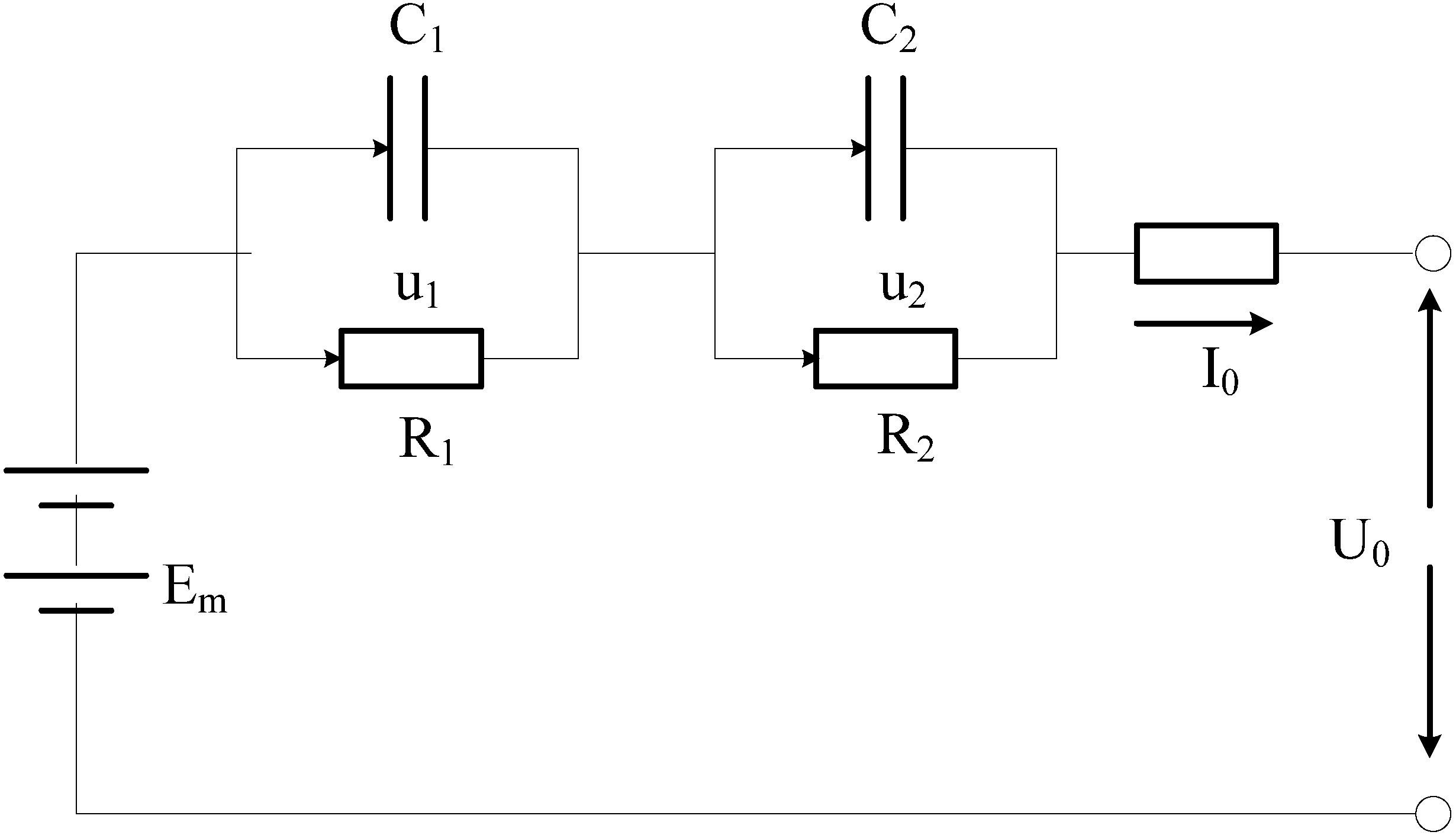
2.3. Battery Model

2.4. Tire Model
| No. | 1 | 2 | 3 | 4 | 5 | 6 | 7 | 8 | ||||
|---|---|---|---|---|---|---|---|---|---|---|---|---|
| ai | −21.3 | 1144 | 49.6 | 226 | 0.069 | −0.006 | 0.056 | 0.486 | ||||
| No. | 1 | 2 | 3 | 4 | 5 | 6 | 7 | 8 | 9 | 10 | 11 | 12 |
| bi | −22.1 | 1011 | 1078 | 1.82 | 0.208 | 0 | −0.354 | 0.707 | 0.028 | 0 | 14.8 | 1.122 |
3. Acceleration Slip Regulation Control Strategy
3.1. Analysis of Control Tasks
3.2. Slip Ratio Control
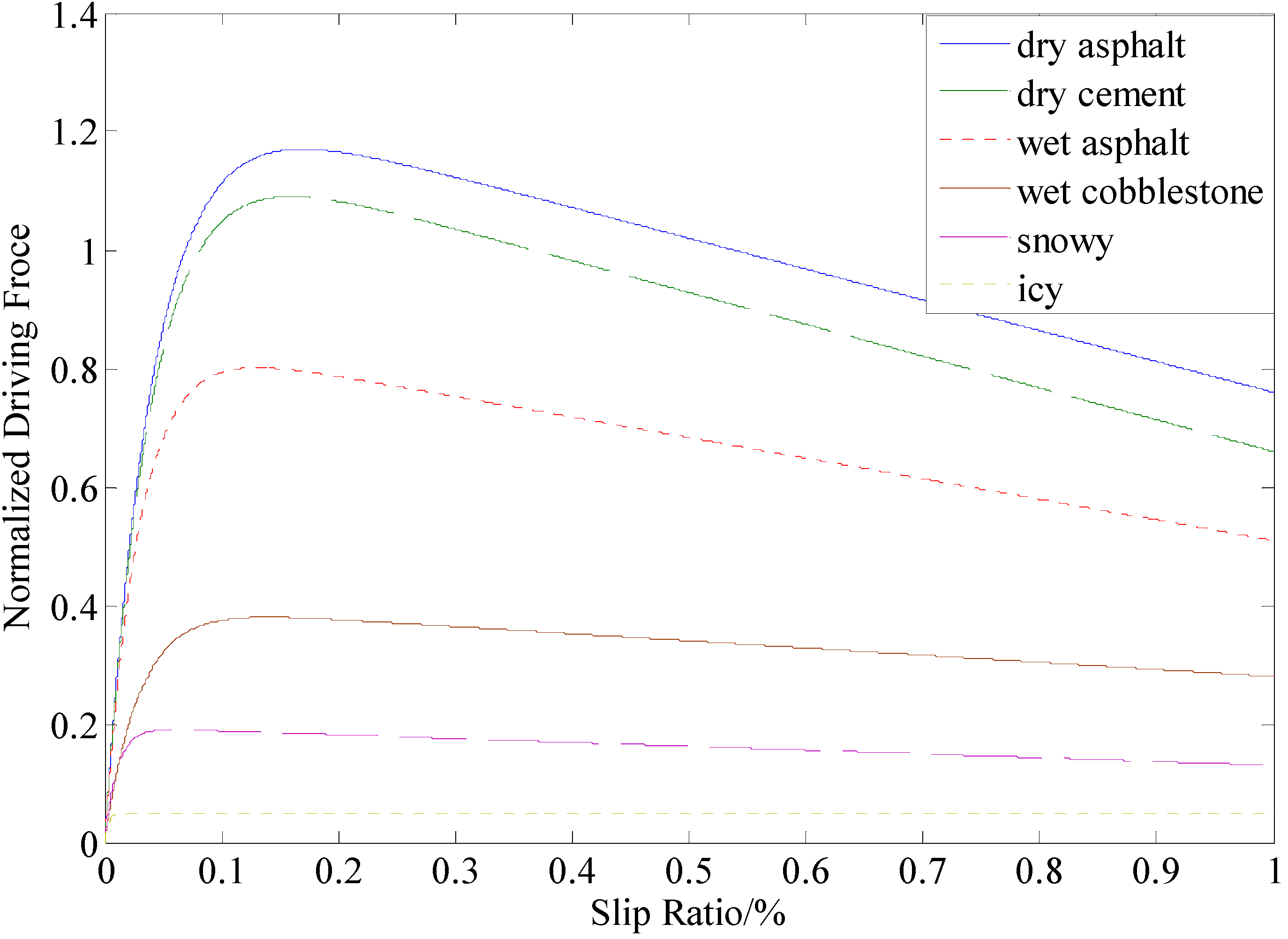
3.2.1. Target Slip Ratio for Acceleration Slip Regulation
| No. | Road condition | C1 | C2 | C3 | λopt | μ(λopt) | μ(λ0)/μ(λopt) |
|---|---|---|---|---|---|---|---|
| 1 | Dry asphalt | 1.2801 | 23.990 | 0.5200 | 0.17 | 1.1700 | 99.74% |
| 2 | Wet asphalt | 0.8570 | 33.822 | 0.3470 | 0.13 | 0.8013 | 99.79% |
| 3 | Dry cement | 1.1973 | 25.168 | 0.5373 | 0.16 | 1.0900 | 99.91% |
| 4 | Wet cobblestone | 0.4004 | 33.708 | 0.1204 | 0.14 | 0.3800 | 99.95% |
| 5 | Snowy | 0.1946 | 94.129 | 0.0646 | 0.06 | 0.1906 | 97.01% |
| 6 | Icy | 0.0500 | 306.39 | 0.0010 | 0.03 | 0.0500 | 99.7% |

3.2.2. The Control Method of Slip Ratio
3.3. Yaw Rate Control
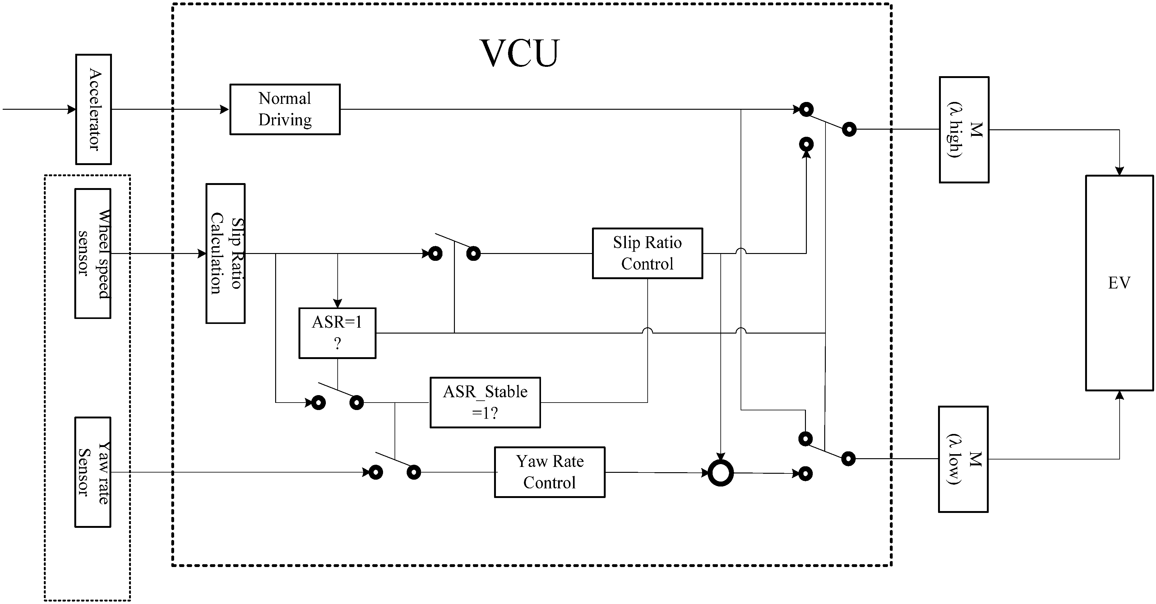
3.4. Coordination Control for Acceleration Slip Regulation
3.4.1. Properties and Coordination Requirement
3.4.2. Adjusting and Stable Stage of Slip Ratio Control

3.4.3. The Coordination Control and Implementation

4. Simulation Results and Analysis
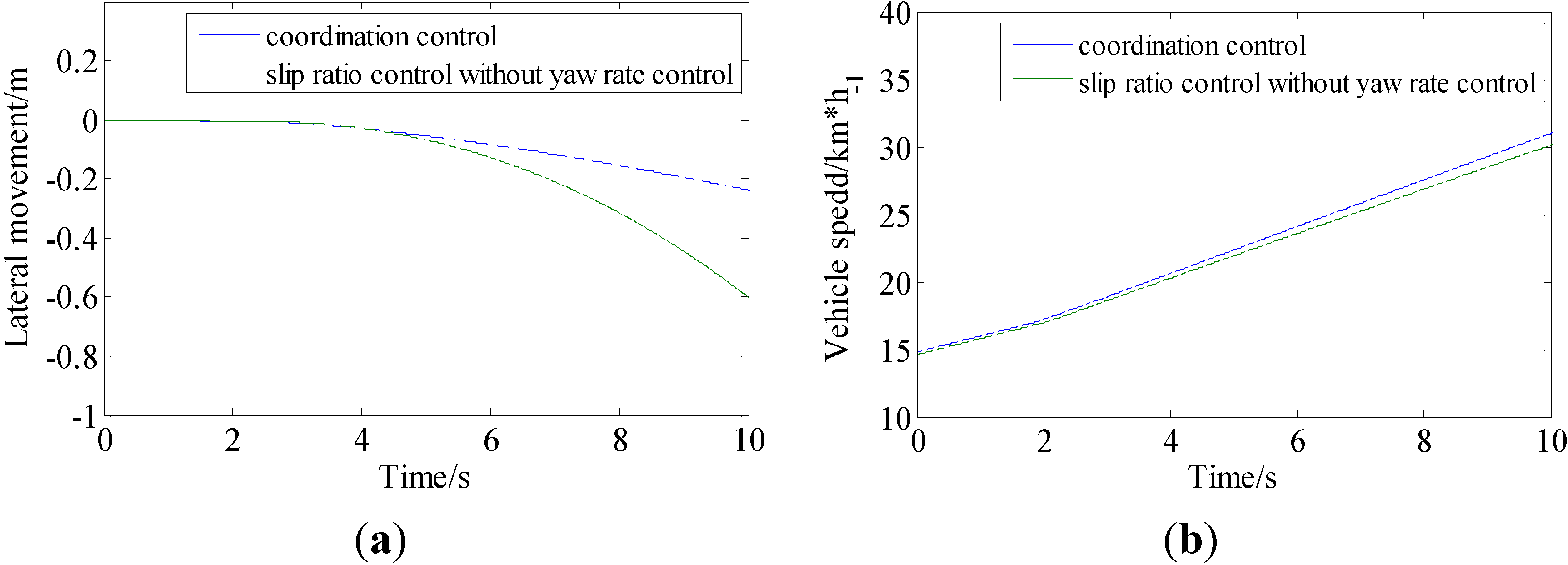
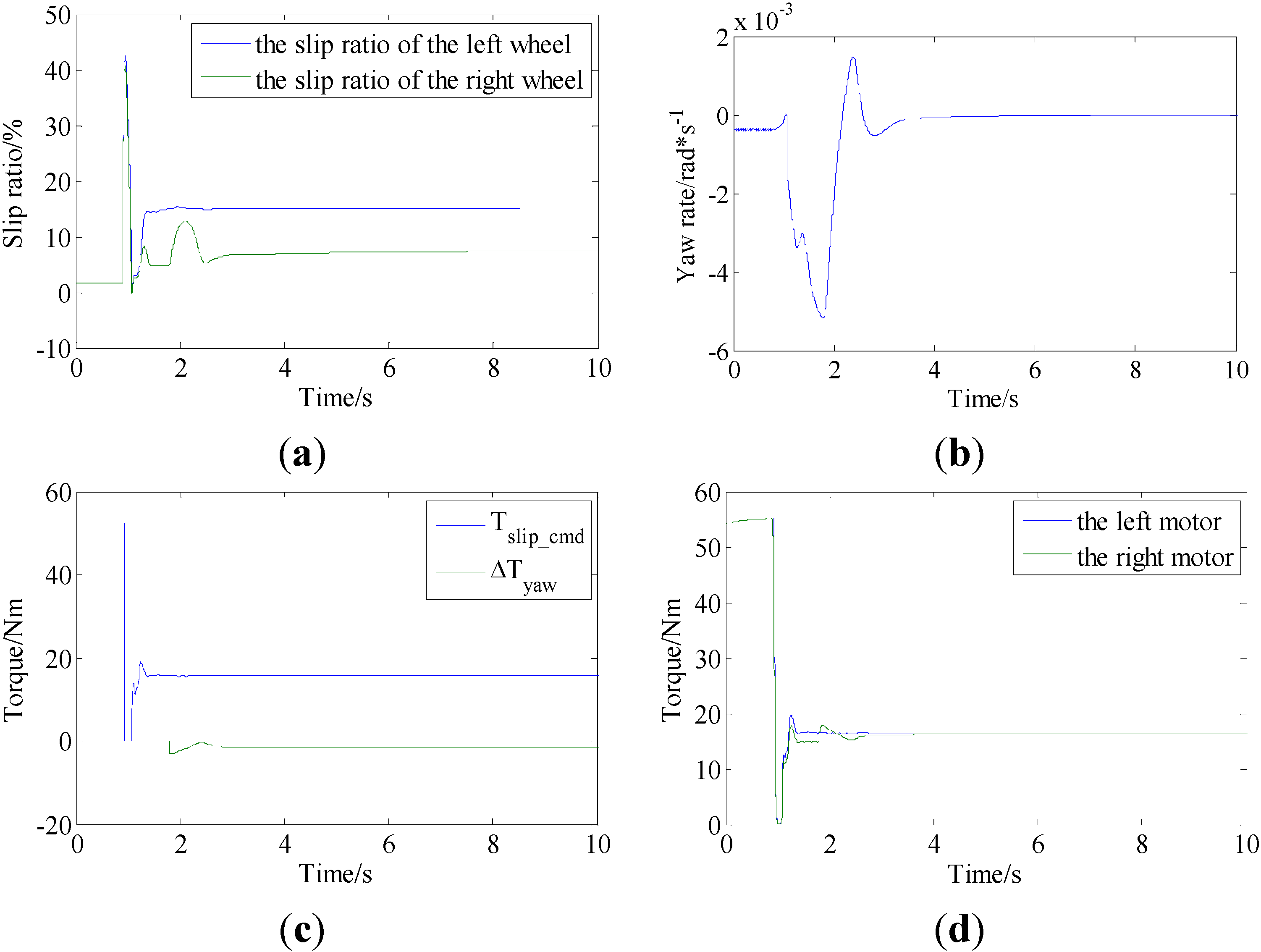
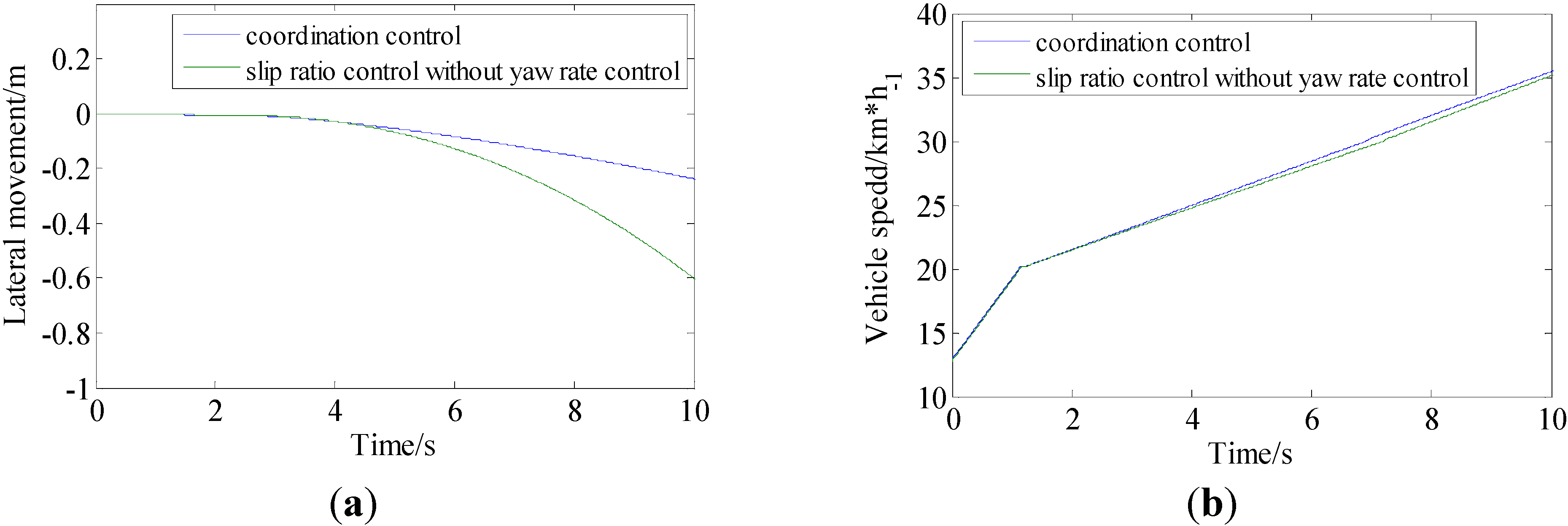
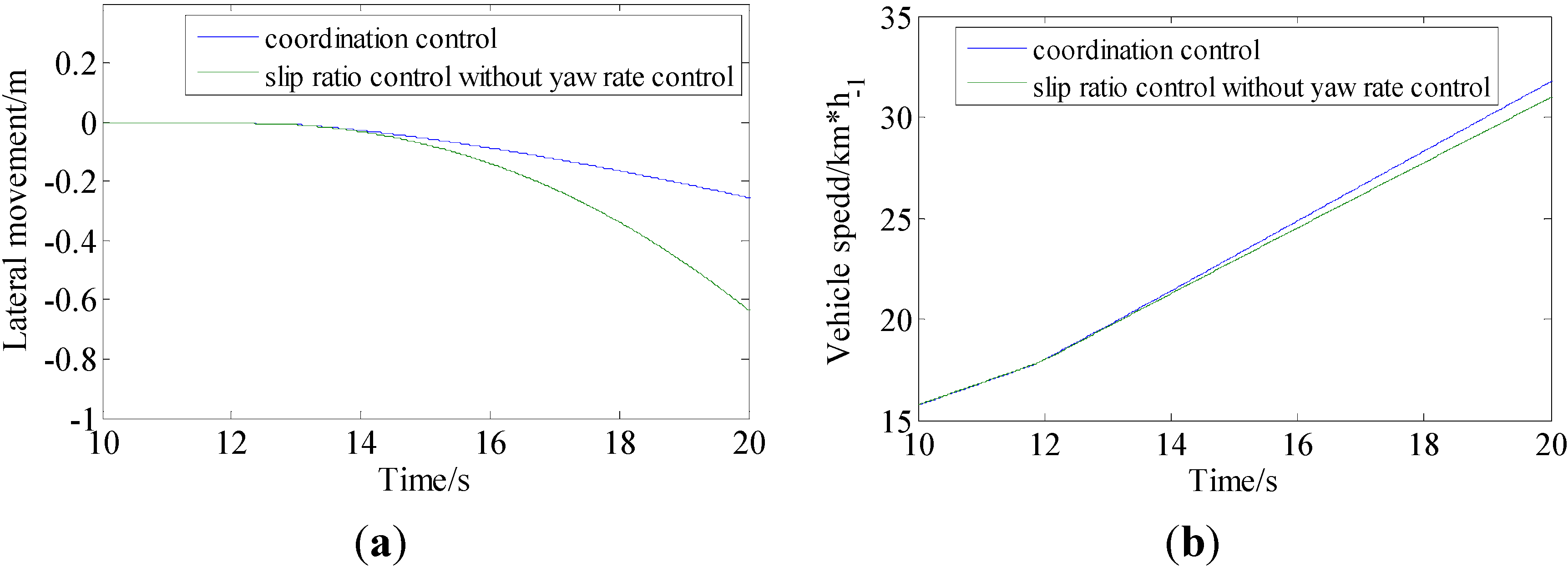
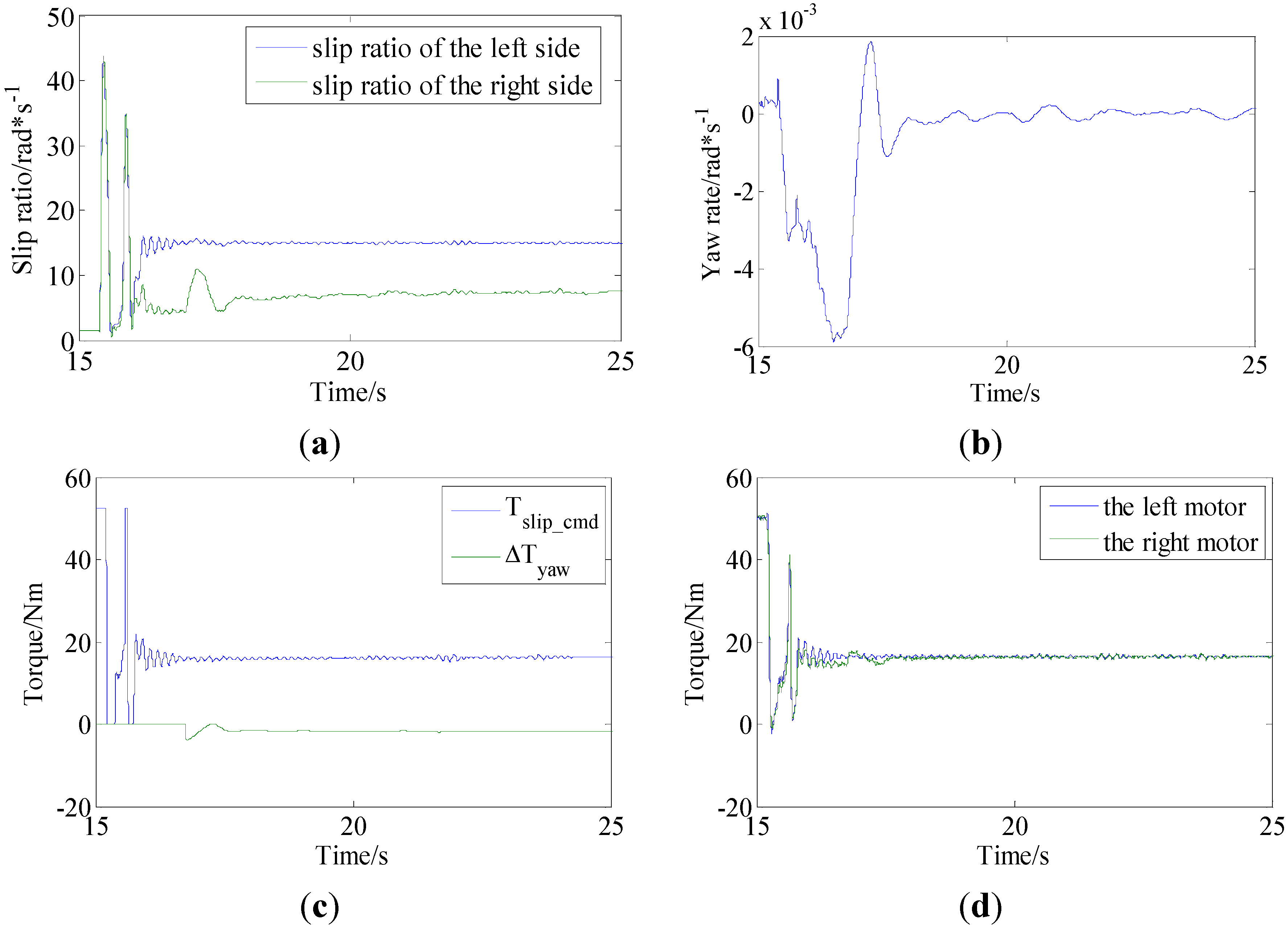
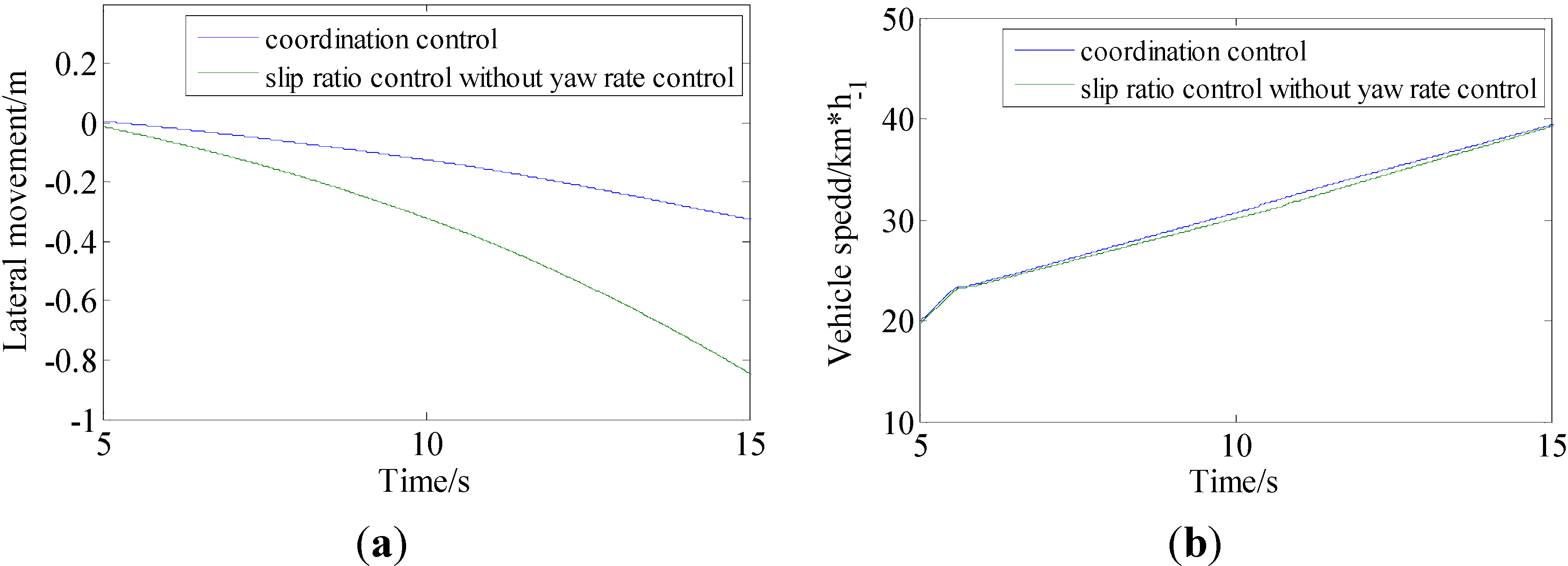
4.1. Simulation of Low Friction Road Conditions


| Performance | Normal strategy | Proposed strategy | Improvement |
|---|---|---|---|
| Average acceleration | 0.455 m/s2 | 0.483 m/s2 | 6.1% |
| Lateral movement | 0.59 m | 0.24 m | 59.3% |
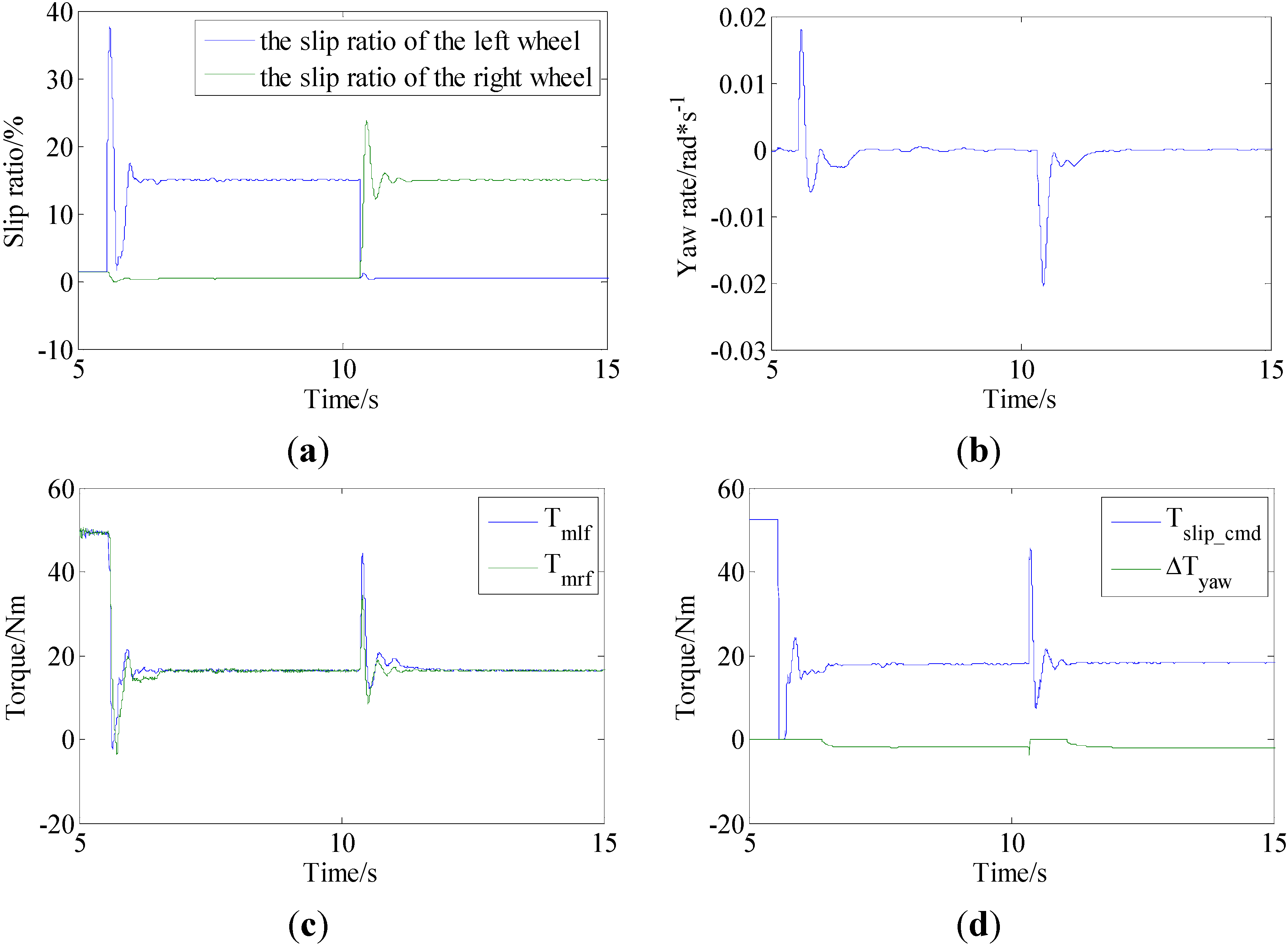
4.2. Simulation of Varying Friction Coefficient Road Conditions


| Performance | Normal strategy | Proposed strategy | Improvement |
|---|---|---|---|
| Average acceleration | 0.452 m/s2 | 0.475 m/s2 | 5.1% |
| Lateral movement | 0.66 m | 0.26 m | 60.6% |
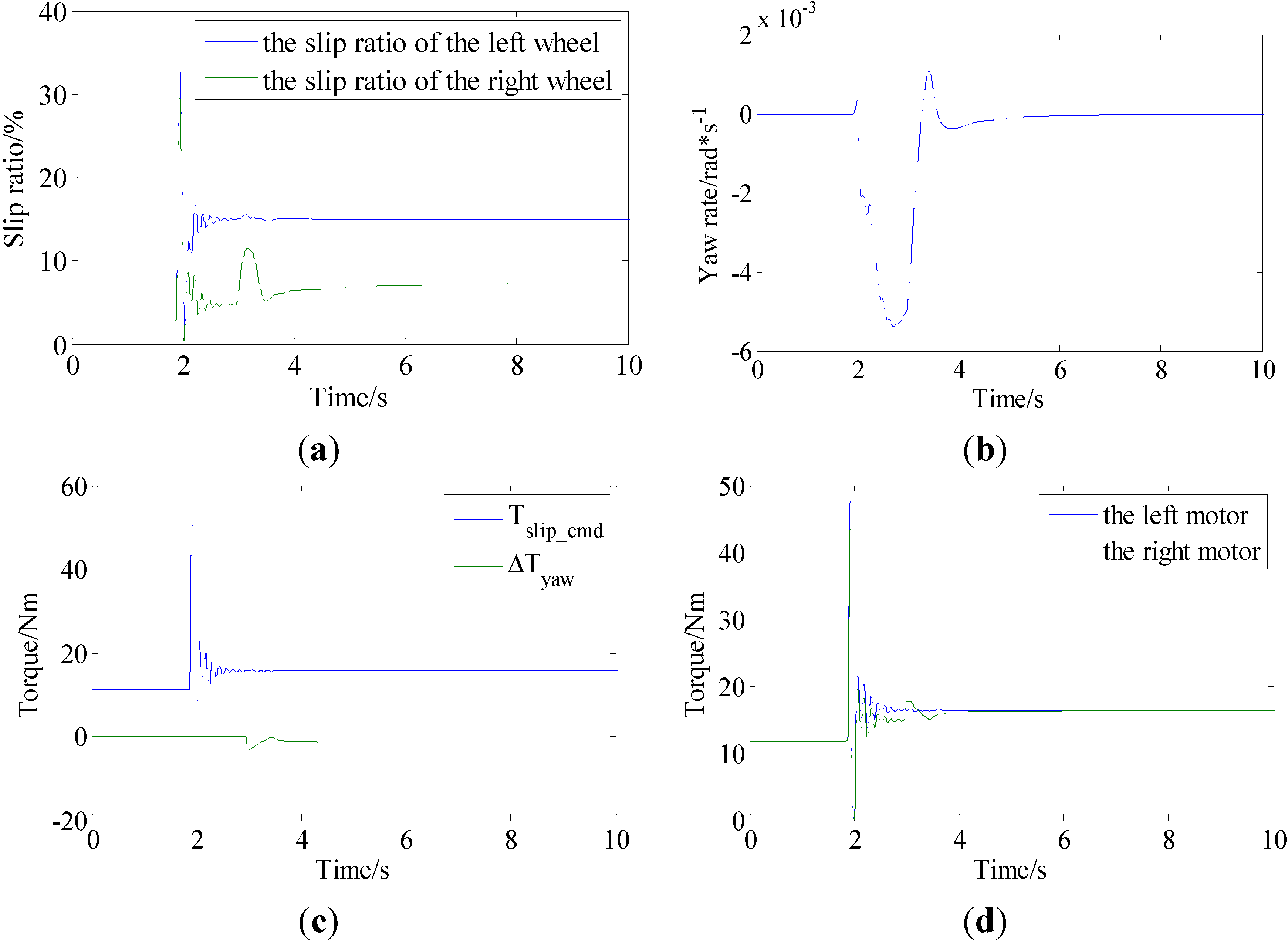
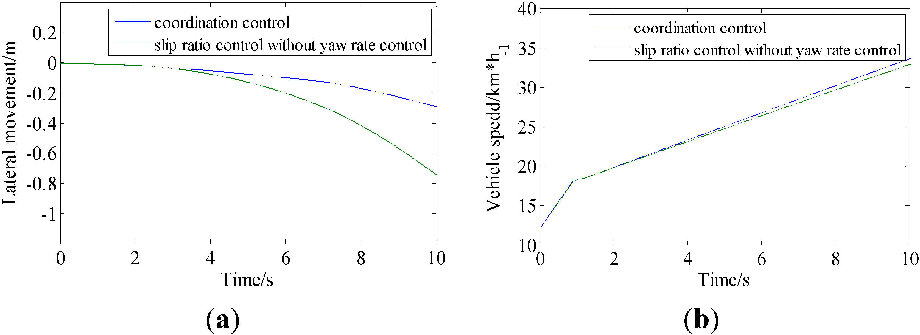
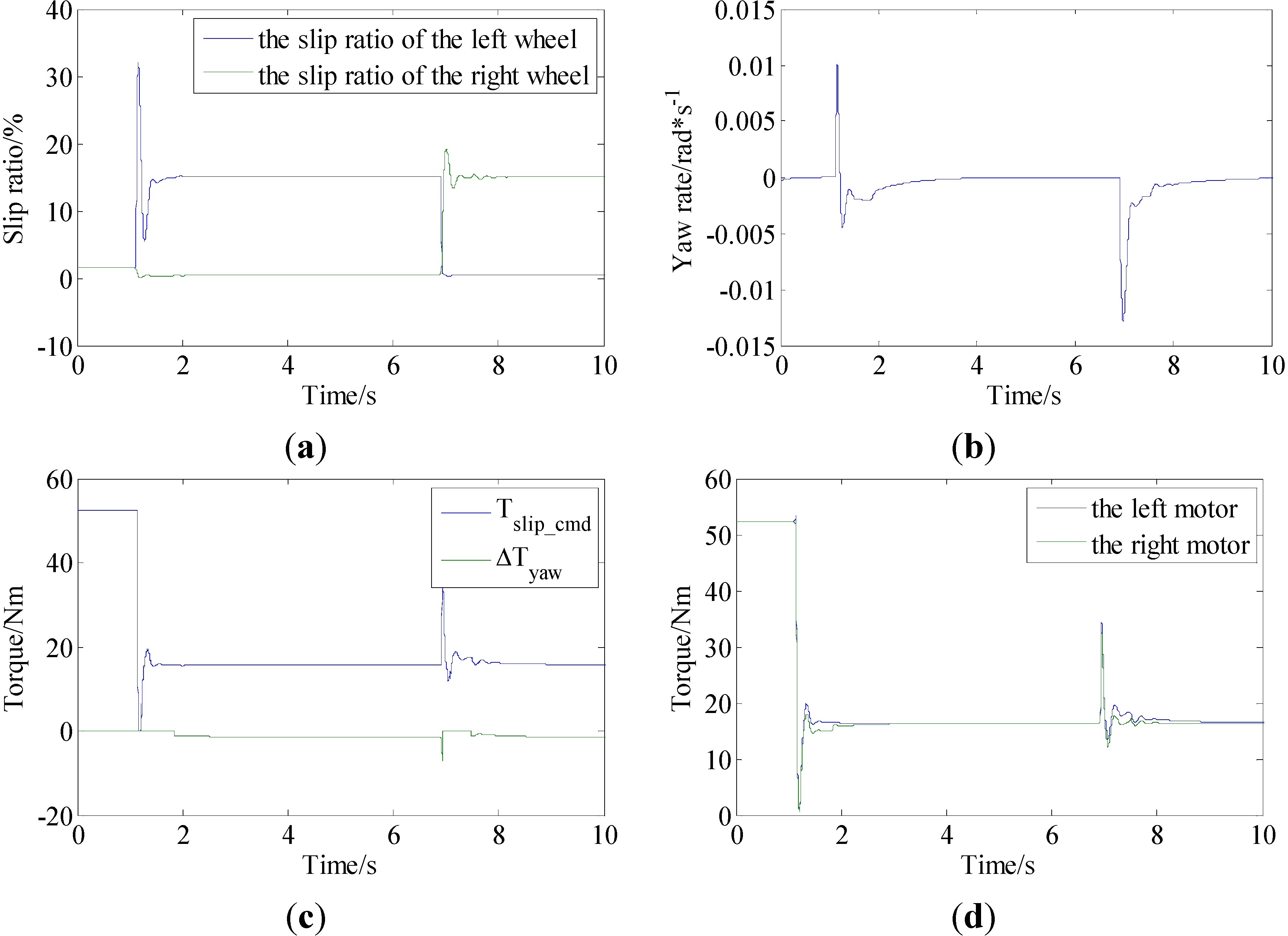
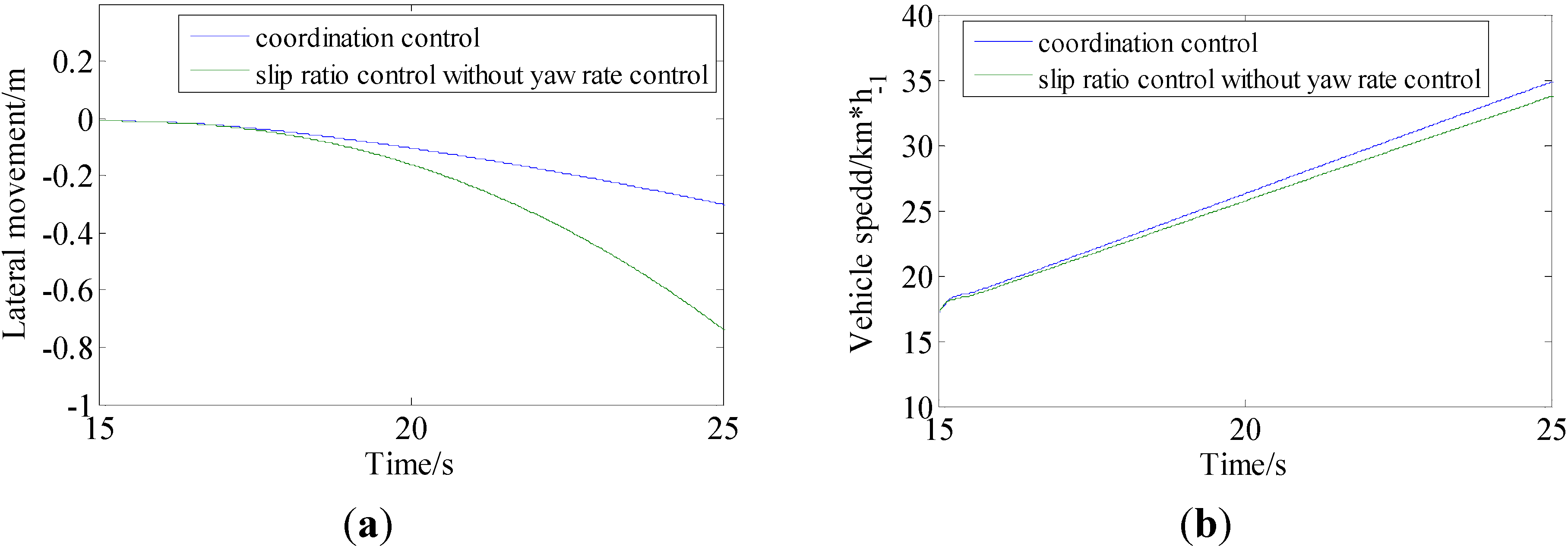
4.3. Simulation of Variation Split-μ Road Conditions


| Performance | Normal strategy | Proposed strategy | Improvement |
|---|---|---|---|
| Average acceleration | 0.475 m/s2 | 0.484 m/s2 | 1.9% |
| Lateral movement | 0.74 m | 0.29 m | 60.8% |
5. Experimental Results and Analysis
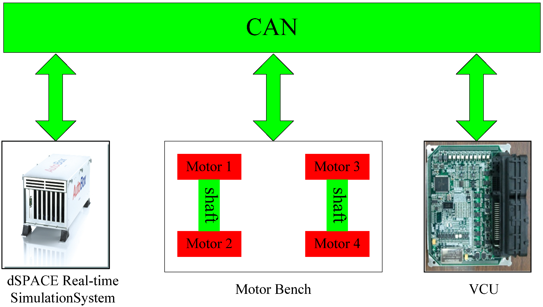
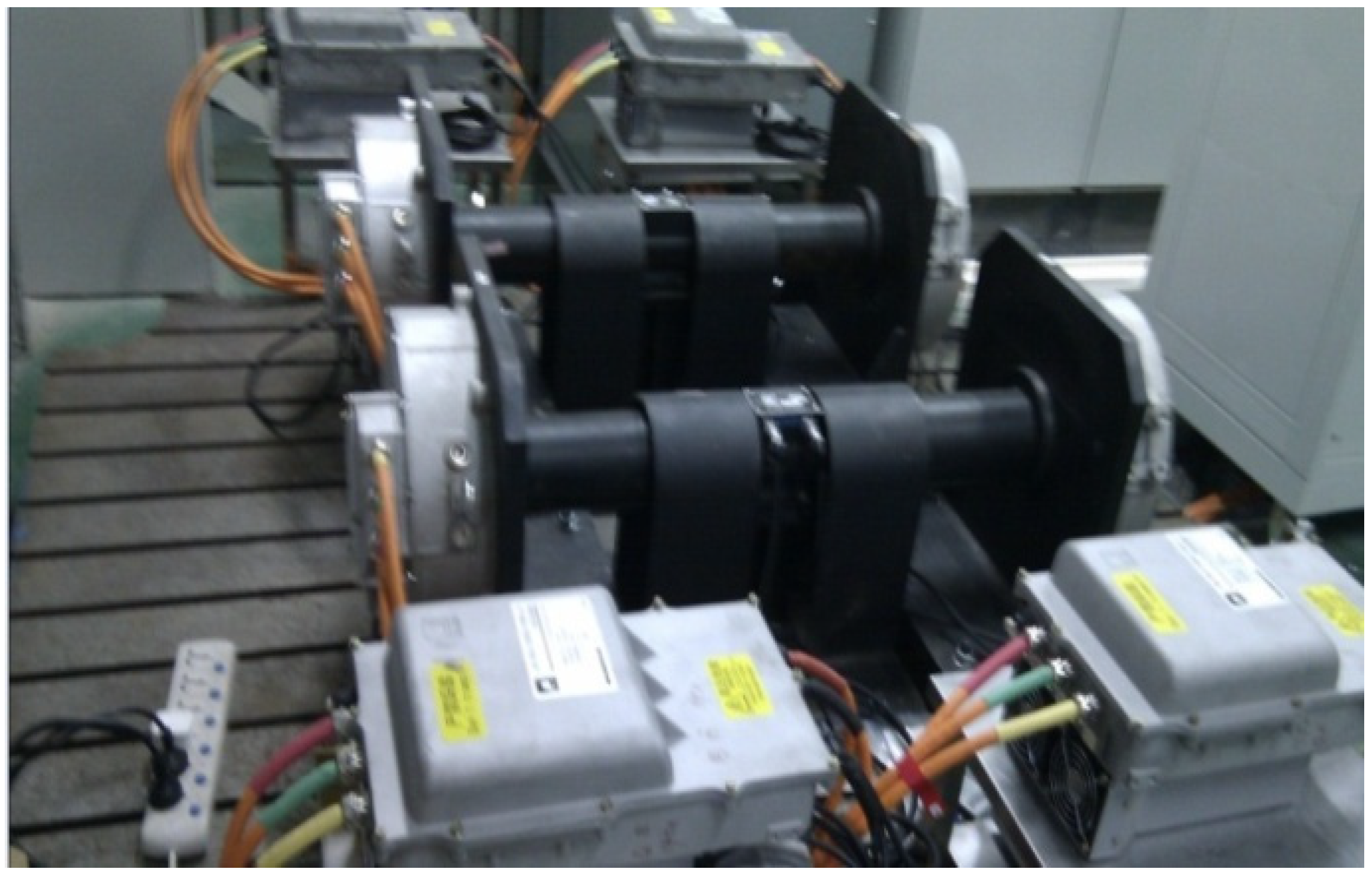
5.1. Hardware-in-Loop Test Bench


| Motor parameters | Rated power | 10 kW |
| Maximum speed | 4,000 rpm | |
| Rated torque | 76.4 Nm | |
| Torque control accuracy | >99% | |
| Torque responsive time | 20 ms | |
| Measurement accuracy | Torque | 0.2% |
| Rotate speed | 0.5 r/min | |
| Sample frequency | 2 ms |
5.2. Experiment Results and Analysis
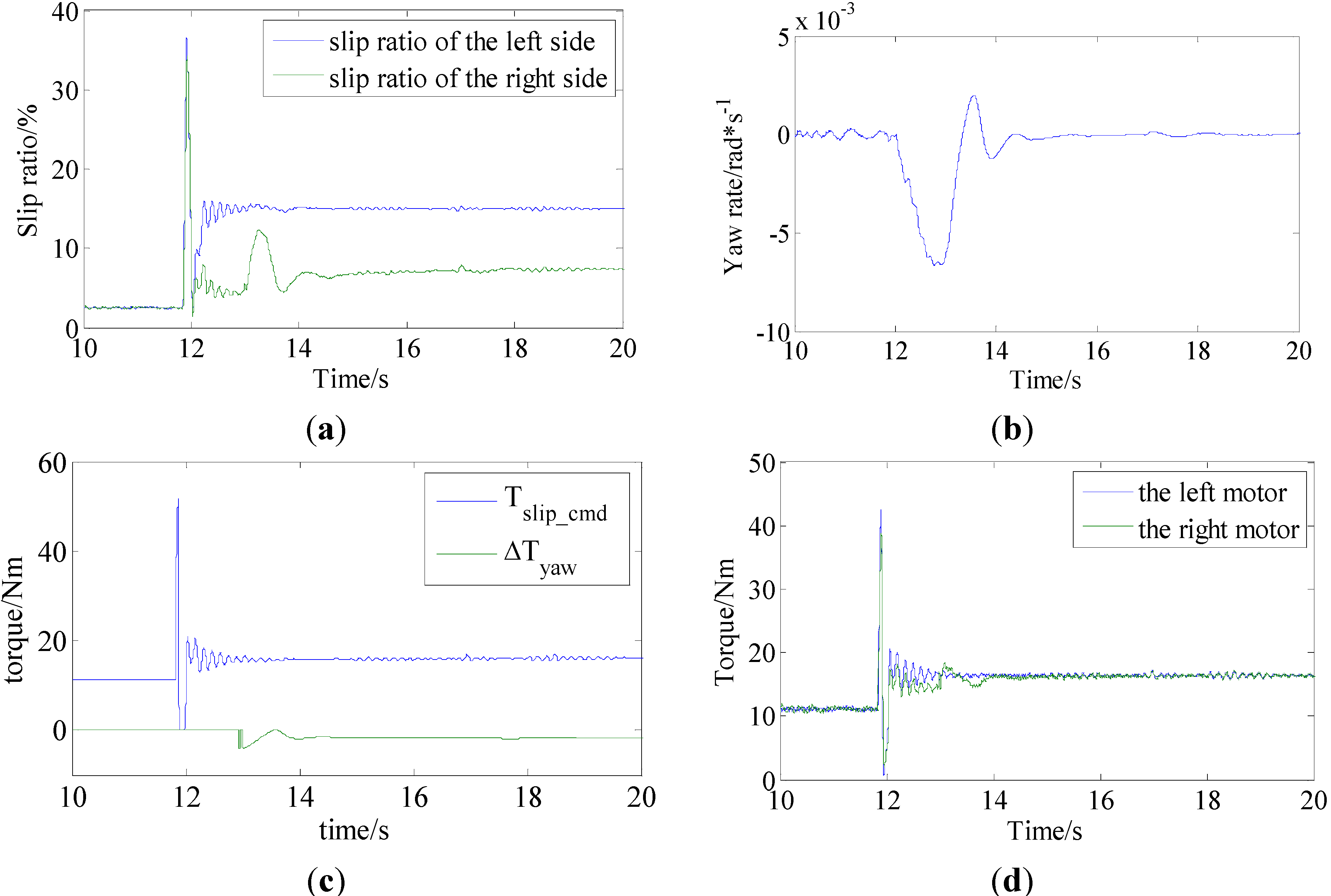
5.2.1. Hardware-in-Loop Experiment of a Low Friction Road


| Performance | Normal strategy | Proposed strategy | Improvement |
|---|---|---|---|
| Average acceleration | 0.441 m/s2 | 0.473 m/s2 | 7.3% |
| Lateral movement | 0.63 m | 0.26 m | 58.7% |
5.2.2. Hardware-in-Loop Experiment of Varying Friction Coefficient Road Conditions


| Performance | Normal strategy | Proposed strategy | Improvement |
|---|---|---|---|
| Average acceleration | 0.453 m/s2 | 0.475 m/s2 | 5% |
| Lateral movement | 0.73 m | 0.29 m | 60.3% |
5.2.3. Hardware-in-Loop Experiment of Varying Split-μ Road Conditions


| Performance | Normal strategy | Proposed strategy | Improvement |
|---|---|---|---|
| Average acceleration | 0.475 m/s2 | 0.475 m/s2 | 0% |
| Lateral movement | 0.84 m | 0.32 m | 61.9% |
6. Conclusions
- (1)
- The proposed slip ratio control method could keep the slip ratio stable at the optimal point when the acceleration slip regulation was activated.
- (2)
- A yaw rate could be generated by the torque difference between the motors due to the different torque errors, which affects the straight line driving performance. The proposed yaw rate control could reduce the yaw rate and lateral movement.
- (3)
- The coordination control of the slip ratio control and yaw rate control was proposed, based on an analysis of the priorities and features of the two control processes. The coordination control could prevent the vibration of the control effects.
- (4)
- Simulations and hardware-in-loop experiments have been carried out under different road conditions, and the effectiveness of the strategy has been verified. Compared with normal acceleration slip regulation, the proposed strategy could improve the acceleration performance on low friction roads and improve the straight line driving performance during the acceleration slip regulation of the vehicle.
Acknowledgments
Author Contributions
Conflicts of Interest
References
- Nagai, M. The perspectives of research for enhancing active safety based on advanced control technology. Veh. Syst. Dyn. 2007, 45, 413–431. [Google Scholar] [CrossRef]
- Chau, K.T.; Chan, C.C.; Liu, C. Overview of permanent-magnet brushless drives for electric and hybrid electric vehicles. IEEE Trans. Ind. Electron. 2008, 55, 2246–2257. [Google Scholar] [CrossRef] [Green Version]
- Hori, Y. Future vehicle driven by electricity and control-Research on four-wheel-motored “UOT electric march II”. IEEE Trans. Ind. Electron. 2004, 51, 954–962. [Google Scholar] [CrossRef]
- Liu, W.; He, H.; Peng, J. Driving control research for longitudinal dynamics of electric vehicles with independently driven front and rear wheels. Math. Probl. Eng. 2013, 2013. [Google Scholar] [CrossRef]
- Jalali, K.; Uchida, T.; McPhee, J.; Lambert, S. Development of a fuzzy slip control system for electric vehicles with in-wheel motors. SAE Int. J. Alt. Power. 2012, 1, 46–64. [Google Scholar] [CrossRef]
- Gou, J.F.; Zhang, B.; Wang, L.F.; Zhang, J.Z. Acceleration slip regulation of electric vehicles. In Proceedings of the 2010 International Conference on Logistics Engineering and Intelligent Transportation Systems, Wuhan, China, 26–28 November 2010.
- Zhao, Z. Study of acceleration slip regulation strategy for four wheel drive hybrid electric car. Chin. J. Mech. Eng. 2011, 47, 83–98. [Google Scholar] [CrossRef]
- Goran, V.; Karlo, G.; Stjepan, B. Experimental testing of a traction control system with on-line road condition estimation for electric vehicles. In Proceedings of the 21st Mediterranean Conference on Control & Automation (MED), Chania, Crete, Greece, 25–28 June 2013.
- He, H.; Peng, J.K.; Rui, X.; Hao, F. An acceleration slip regulation strategy for four-wheel drive electric vehicles based on sliding mode control. Energies 2014, 7, 3748–3763. [Google Scholar] [CrossRef]
- Lin, C.; Cheng, X.Q. A traction control strategy with an efficiency model in a distributed driving electric vehicle. Sci. World J. 2014, 2014. [Google Scholar] [CrossRef]
- Yin, G.D.; Wang, S.B.; Jin, X.J. Optimal slip ratio based fuzzy control of acceleration slip regulation for four-wheel independent driving electric vehicles. Math. Probl. Eng. 2013, 2013. [Google Scholar] [CrossRef]
- Subudhi, B.; Ge, S.S. Sliding-mode-observer-based adaptive slip rate control for electric and hybrid vehicles. IEEE Trans. Intell. Trans. Syst. 2012, 13, 1617–1626. [Google Scholar] [CrossRef]
- Yin, D.; Oh, S.; Hori, Y. A novel traction control for EV based on maximum transmissible torque estimation. IEEE Trans. Ind. Electron. 2009, 56, 2086–2094. [Google Scholar] [CrossRef]
- Hori, Y.; Toyoda, Y.; Tsuruoka, Y. Traction control of electric vehicle: Basic experimental results using the test EV “UOT electric march”. Ind. Appl. IEEE Trans. 1998, 34, 1131–1138. [Google Scholar] [CrossRef]
- Tora, A.; Ryota, S.; Takeshi, F.; Jun, T. A study of novel traction control for electric motor driven vehicle. In Proceedings of the Power Conversion Conference, Nogaya, Japan, 2–5 April 2007.
- Zhao, Z. Torque adaptive traction control for distributed drive electric vehicle. Chin. J. Mech. Eng. 2013. [Google Scholar] [CrossRef]
- Gillespie, T. Fundamentals of Vehicle Dynamic; SAE Publications: Warrendale, PA, USA, 1992; pp. 8–18. [Google Scholar]
- Mirzaeinejad, H.; Mirzaei, M. A novel method for non-linear control of wheel slip in anti-lock braking systems. Control Eng. Pract. 2010, 18, 918–926. [Google Scholar] [CrossRef]
- Tahami, F.; Kazemi, R.; Farhanghi, S. A novel driver assist stability system for all-wheel-drive electric vehicles. IEEE Trans. Veh. Technol. 2003, 52, 683–692. [Google Scholar] [CrossRef]
- Wang, R.; Chen, Y.; Feng, D.; Huang, X.Y.; Wang, J.M. Development and performance characterization of an electric ground vehicle with independently actuated in-wheel motors. J. Power Sources 2011, 196, 3962–3971. [Google Scholar] [CrossRef]
- He, Y.; Liu, X.T.; Zhang, C.B.; Chen, Z.H. A new model for State-of-Charge (SOC) estimation for high-power Li-ion batteries. Appl. Energy 2013, 101, 808–814. [Google Scholar] [CrossRef]
- Pacejka, H.B.; Bakker, E. The magic formula tyre model. Veh. Syst. Dyn. 1992, 21, 1–18. [Google Scholar] [CrossRef]
- Kong, L. Key Control Technologies Research and Development of Anti-lock Braking System for Industrialization. Ph.D. Thesis, Tsinghua University, Beijing, China, 2006. [Google Scholar]
- Harifi, A.; Aghagolzadeh, A.; Alizadeh, G.; Sadeghi, M. Designing a sliding mode controller for slip control of antilock brake systems. Transp. Res. Part C: Emerg. Technol. 2008, 16, 731–741. [Google Scholar] [CrossRef]
© 2015 by the authors; licensee MDPI, Basel, Switzerland. This article is an open access article distributed under the terms and conditions of the Creative Commons Attribution license (http://creativecommons.org/licenses/by/4.0/).
Share and Cite
Wu, L.; Gou, J.; Wang, L.; Zhang, J. Acceleration Slip Regulation Strategy for Distributed Drive Electric Vehicles with Independent Front Axle Drive Motors. Energies 2015, 8, 4043-4072. https://doi.org/10.3390/en8054043
Wu L, Gou J, Wang L, Zhang J. Acceleration Slip Regulation Strategy for Distributed Drive Electric Vehicles with Independent Front Axle Drive Motors. Energies. 2015; 8(5):4043-4072. https://doi.org/10.3390/en8054043
Chicago/Turabian StyleWu, Lingfei, Jinfang Gou, Lifang Wang, and Junzhi Zhang. 2015. "Acceleration Slip Regulation Strategy for Distributed Drive Electric Vehicles with Independent Front Axle Drive Motors" Energies 8, no. 5: 4043-4072. https://doi.org/10.3390/en8054043