Article

Locational Pricing to Mitigate Voltage Problems Caused by High PV Penetration

1
Division Electrical Energy and Computer Architectures, Department of Electrical Engineering, Katholieke Universiteit Leuven (ELECTA, KU Leuven), Kasteelpark Arenberg 10, bus 2445, 3001 Leuven, Belgium
2
Vlaamse Instelling voor Technologisch Onderzoek (VITO), Boerentang 200, 2400 Mol, Belgium
*
Author to whom correspondence should be addressed.
Energies 2015, 8(5), 4607-4628; https://doi.org/10.3390/en8054607
Submission received: 17 February 2015 / Revised: 11 May 2015 / Accepted: 12 May 2015 / Published: 21 May 2015
(This article belongs to the Collection Smart Grid)

Abstract

:
In this paper, a locational marginal pricing algorithm is proposed to control the voltage in unbalanced distribution grids. The increasing amount of photovoltaic (PV) generation installed in the grid may cause the voltage to rise to unacceptable levels during periods of low consumption. With locational prices, the distribution system operator can steer the reactive power consumption and active power curtailment of PV panels to guarantee a safe network operation. Flexible loads also respond to these prices. A distributed gradient algorithm automatically defines the locational prices that avoid voltage problems. Using these locational prices results in a minimum cost for the distribution operator to control the voltage. Locational prices can differ between the three phases in unbalanced grids. This is caused by a higher consumption or production in one of the phases compared to the other phases and provides the opportunity for arbitrage, where power is transferred from a phase with a low price to a phase with a high price. The effect of arbitrage is analyzed. The proposed algorithm is applied to an existing three-phase four-wire radial grid. Several simulations with realistic data are performed.

1. Introduction

The electricity grid is going through a transition period. A high penetration of PV panels and the ongoing electrification of the transport system requires new strategies for the operation and management of the electricity grid. Typically, the high-power injection of PV panels does not coincide with periods of high demand. The resulting high reverse power flow can cause a significant rise in the grid voltage. The maximum amount of PV generation that can be connected to a low-voltage (LV) network is typically limited by this voltage rise [1,2]. In current regulations, a PV panel has to disconnect from the distribution grid as soon as the maximum voltage is reached. However, this can lead to unnecessary curtailed green energy to keep the voltage within limits. Traditionally, distribution system operators (DSOs) are responsible for keeping the grid voltage within limits, and today, more advanced methods may be needed to control the grid voltage.
Different control strategies have been proposed to control the grid voltage and to avoid damage to the grid. One method consists of PV panels that curtail part of the active power to reduce the voltage [1,2]. Another option is to use the remaining inverter capacity of a PV panel to do reactive voltage control [36]. Furthermore, flexible loads, like electric vehicles, can increase or decrease their consumption to regulate the grid voltage [7]. All of these methods are effective at managing the grid voltage, but do not give a real-time incentive to the customers to control the voltage. Furthermore, these strategies should be combined to achieve optimal grid voltage control, and the most cost-effective option should be chosen to comply with the voltage limits.
Real-time pricing is a well-known demand-side management technique. When real-time pricing is applied, electricity consumers are charged with prices that can vary over short time intervals. It can be very effective in shaping the customers’ demand [8] and can be used to keep the total consumption level below the power generation capacity [9]. It is an incentive that is offered by the grid operator and is assumed to be accepted by the users [10,11]. In this work a real-time pricing strategy is used to control the grid voltage. A community of cooperative consumers is assumed. In contrast to the methods described in [8,9,12], the tariff will not depend on the power, but on the grid voltage. The distribution system operator can adapt the real-time energy price to keep the voltage within limits. This price will give an incentive to inject or consume reactive power to control the voltage or, if necessary, to curtail active power or adapt the consumption of the flexible load. The most cost-effective solution will be obtained. The prices are defined by a distributed gradient algorithm, based on a two-way communication system. The pricing is applied to unbalanced distribution networks, which requires special care due to the neutral point shifting. In previous work, this pricing strategy was tested for active power only [13]. In this work, incentives will be given for reactive voltage control, as well.
Centralizing all of the information to obtain the optimal setpoints or the real-time prices should be omitted to protect the privacy of the customers [9,12,1416]. Several distributed algorithms are proposed to schedule loads without centralizing all of the information. In [9,12,14], the distributed algorithm is based on Lagrange relaxation. The work in [15] describes distributed algorithms that use Q-learning and Lyapunov optimization. In [16], a distributed algorithm based on a non-cooperative Stackelberg game is presented. In our work, network prices are defined in a distributed way by means of Lagrange relaxation.
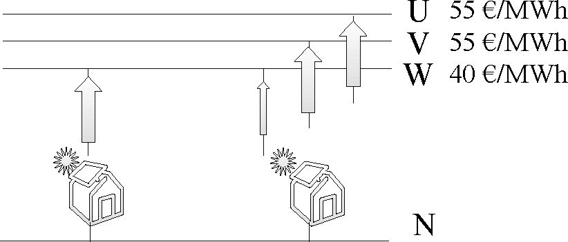
Finally, arbitrage will be analyzed. Arbitrage is possible when the same asset, in this case energy, does not trade at the same price at different locations. PV generation is not necessarily spread equally across the three phases. This can lead to higher voltages in the phase with the highest power production [17] and, therefore, a lower price for energy that is injected into this phase. When there is a price difference for the energy in the three different phases, at the same location, power can be transferred from the phase with the lowest price to the phase with the highest price. This can be done with adapted PV inverters. PV inverters rarely operate at their maximal power production. If a three-phase PV inverter consists of three single-phase inverters with a common DC-bus, it is possible for the majority of the produced power to be injected into the phase with the highest power consumption or to transfer power from highly loaded to less loaded phases, without overloading the PV inverter. This principle is illustrated in Figure 1.
This paper is structured as follows: In Section 2, the distribution grid used in the simulation results is described, and special attention is given to effects in unbalanced grids, because these will have implications on the locational grid prices. Section 3 describes the system model that defines the optimal response of the flexible loads and PV units, and Section 4 elaborates on the distributed pricing strategy that results in the same response as the optimization problem, which was defined in Section 3. Finally, Section 5 presents some results and shows how PV panels, flexible loads and three-phase PV inverters that perform arbitrage react to the locational prices.

2. Simulated Network

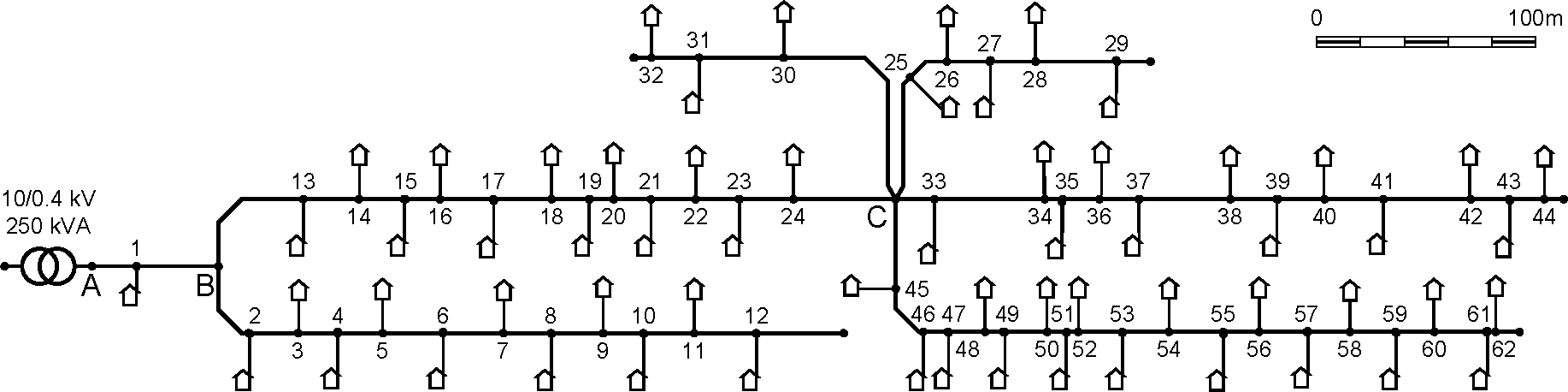
An existing three-phase four-wire radial distribution system with a TTearthing arrangement in Belgium was used for the simulations. The network consists of 62 customers and is depicted in Figure 2. This network is a semi-urban reference network used in the LINEARproject [18] and has been studied often [4,7,19,20].
The main feeder cables are of type EAXVB1 kV 4 × 150 mm2, while the cable between Node A and Node B is of type EAXVB 1 kV 4 × 95 mm2. The assumed operating temperature is 45 °C. All households have a single-phase connection, except households 41 and 62, which have a three-phase connection to the network. The households with a single-phase connection are spread equally across the three phases in the order U,V,W,U,V,W, etc. The voltage at the secondary side of the transformer is considered to be 230 V during no load. All households have a PV installation. The PV inverter rating of the households connected to Phases U and V equals 2.2 kW, while the households connected to Phase W have a rating of 3.3 kW. These assumptions will create unbalance in the network. The households with a three-phase connection have a three-phase PV installation with a rating of 6 kW.
A remarkable and important effect in three-phase four-wire grids is the neutral point shifting [21]. When a single-phase load consumes active or reactive power, a current will flow through the neutral conductor. This results in a voltage drop over the impedance of the neutral conductor, and the neutral voltage experienced by all customers will shift. As a consequence of the neutral shift, reactive power absorption in Phase U significantly increases the phase voltage of Phase W and decreases the phase voltage of Phase V. To decrease the voltage in one phase, it can be more beneficial to inject reactive power into another phase than to absorb reactive power into this specific phase itself [4]. This is important for the locational pricing approach that will be developed. When voltage problems occur in one phase, the DSO should give an incentive to inject reactive power into another phase. Another consequence of the neutral shift is that consuming power in one phase will decrease the voltage in this phase, whereas the voltage in the other two phases will slightly increase.
Voltage limits are the major concern when integrating distributed generation in distribution networks. Like in DC power flow models [17], AC models can be approximated with a linear model to describe the influence of PV panels and flexible loads on the voltage magnitude [19,2226]. The voltage at a node m can be approximated by:
| V m | | V m base | + k = 1 N ( μ m , k , i P P k , i + μ m , k , i Q Q k , i )
where:
  • μ m , k , i P is the sensitivity of the voltage magnitude in node m by active power injected at node k into phase i;
  • Pk,i is the active power injected or consumed at node k into/from phase i by a PV panel or a flexible load;
  • μ m , k , i Q is the sensitivity of the voltage magnitude in node m by reactive power injected at node k into phase i;
  • Qk,i is the reactive power injected at node k into phase i by a PV panel;
  • V m base is the voltage at node m due to the uncontrollable load of the households;
  • Vm is the expected voltage at node m;
  • N is the number of nodes.
The voltages are limited between a minimum and a maximum voltage:
V min | V m | V max
where Vmin and Vmax are the minimum and maximum allowed voltages. In this work, Vmin and Vmax are chosen to be ±10% of the nominal voltage of 230 V. The voltages of control points at the end of the feeders have to be monitored and controlled, as these are subject to the largest voltage deviations. These voltages are measured and communicated to the DSO. In this work, Nodes 44 and 62 are these controlled nodes.
Using the linear voltage model described in Constraint (1) has various advantages. First of all, the DSO does not need to know the actual uncontrollable load of the households to approximate the voltage caused by the uncontrollable load alone. Since this could contain privacy-sensitive information, the customers preferably do not share this information in a central instance [10]. If the DSO knows the consumption of the PV panels and of the flexible loads during the voltage measurement, he can calculate the effect that these have on the voltage measurement with the voltage sensitivity factors. With this information, he can then obtain the voltage caused by only the uncontrollable base load V m base, without having information on the uncontrollable household consumption.
The second advantage is that the voltage Constraints (1) and (2) remain an easy to handle convex set. Another advantage is that these sensitivity factors can be approximated based on historic smart meter data, without having information about the exact grid topology [24].
In real-life conditions, the uncontrollable load can vary. The obtained V m base is therefore an estimate of the voltage, caused by only the uncontrollable base load, at the next time step. Furthermore, in the linear model, linearization errors should also be taken into account. It is therefore advised to include a small extra conservative margin in the limits of Constraint (2). Vmin and Vmax can be chosen to be ± 9% of the nominal voltage, whereas the actual limits equal ±10% of the nominal voltage. The magnitude of the linearization errors will depend on the grid topology and the applied load profiles. Typical voltage standards, like EN50160 [27], limit the voltage deviations of the 10-minute mean RMS voltage to ±10%. Therefore, even if the linearization errors would exceed 1%, a regular network price update can compensate quickly for these linearization errors to keep the 10-minute mean RMS voltage within limits, even with inaccurate sensitivity factors [26].

3. System Model

The purpose of the DSO is to keep the voltage within limits in an optimal way, without hindering the normal market operation. To do this, it will have to steer the consumption of flexible loads and single-and three-phase PV panels.
The flexible consumption is modeled by utility functions. The utility function reflects the customer satisfaction for the consumption of their flexible loads. The higher their satisfaction, the higher the price they are willing to pay for the requested energy. In this work, quadratic utility functions are considered, which are one of the most used utility functions [9,2830]:
U ( P k , i fiex ) = ω k P k , i flex β k 2 ( P k , i flex ) 2 for 0 P k , i flex P k max
where:
  • P k , i flex is the flexible power consumption of the load connected to node k at phase i;
  • βk and ωk are confidential parameters characterizing customer types;
  • P k max is the maximal consumption of the flexible load connected to node k.
For an announced price Λk, each customer determines the optimal P k , i flex from:
min . P k , i flex U ( P k , i flex ) + Λ k P k , i flex
It can be proven that a quadratic utility function leads to a consumption P k , i flex that is linearly dependent on the electricity price [31]. Typically, the available flexibility depends on the time of the day. During the day, consumers are often absent, and the available flexibility is small. In the evening, the amount of flexibility is higher. Therefore, the confidential parameters ωk and βk are chosen, such that a price of 0 €/MWh results in a consumption of 1 kW and a price of 100 €/MWh results in a consumption of 0 kW between 08:00 and 18:00 for all houses with a house number that is a multiple of five. The other houses are assumed to have no available flexibility at that moment. In the evening, the parameters are chosen such that a price of 0 €/MWh results in a consumption of 3 kW and a price of 100 €/MWh results in a consumption of 0 kW for all houses with a number that is a multiple of two. Figure 3 gives a summary of the responsiveness of the loads at different moments. The price Λk is the electricity price charged by the provider. This price consists of the generation cost, the taxes and the fixed network tariffs. Further on in this work, a variable network price will be added to control the grid voltage. The price Λk can differ between providers. For simplicity, all of the households received the same price Λk in this work. However, results can be generalized to a situation where all customers have a different electricity price Λk.
Single-phase PV units will always inject the produced power into their phase of connection. Part of the produced power can be curtailed to support the network, but the PV unit will never consume power. The remaining capacity of the PV inverter can be used to inject or absorb reactive power.
Three-phase PV installations inject power into each of the three phases. The three-phase PV inverter usually injects the same amount of active and reactive power into each phase. However, when the three-phase inverter consists of three single-phase units with a common DC-bus, the unit can inject a different amount of active or reactive power into each phase. This type of inverter is referred to as a balancing inverter.
The DSO will try to optimally steer the flexible loads and PV units to avoid voltage limit violations in the grid. If all of the information of the flexible loads and the PV panels could be centralized at one location, the DSO would solve the following problem:
min . P k , i flex , P PV , curt , Q PV k { θ flex } U ( P k , i flex ) + Λ k P k , i flex + Flexible loads
k { θ 1 } Λ k ( P k , i PV P k , i PV , curt ) + α ( Q k , i PV ) 2 + Single-phase PV
k { θ 3 } i { U , V , W } ( Λ k ( P k , i PV P k , i PV , curt ) + α ( Q k , i PV ) 2 ) Three-phase PV
subj. to
P k , i PV P k , i PV , curt 0 k θ 1
i { U , V , W } ( P k , i PV P k , i PV , curt ) 0 k θ 3
( Q k , i PV ) 2 + ( P k , i PV P k , i PV , curt ) 2 S k , i 2 k θ 1
( Q k , i PV ) 2 + ( P k , i PV P k , i PV , curt ) 2 S k , i 2 k θ 3
V min | V m | V max m N c o n t r
| V m | = | V m base | + k = 1 N ( μ m , k , i P ( P k , i PV + P k , i PV , curt + P k , i flex ) ) + k = 1 N μ m , k , i Q Q k , i PV
where:
  • θflex is the set of all customers with a flexible load unit;
  • θ1 is the set of all customers with a single-phase PV unit;
  • θ3 is the set of all customers with a three-phase PV unit;
  • P k , i PV P k , i PV , curt is the net injected power into phase i of the PV panel connected at node k; for a single-phase PV unit, P k , i PV is the total produced power; for a three-phase unit, P k , i PV is one third of the total produced power; part of the produced power can be curtailed P k , i PV , curt;
  • Q k , i PV is the reactive power injected/absorbed by the PV panel connected at node k into phase i;
  • Sk,i is the inverter rating of the PV unit connected at node k to phase i; for a three-phase unit Sk,i is one third of the total three-phase inverter rating;
  • α is a parameter to penalize reactive power injection or absorption by a PV panel;
The objective function consists of three terms. The first term Equation (5) maximizes the utility of the flexible loads. The second term Equation (6) reflects the income of the single-phase PV units. The units get a price of Λk for the injected power and have a decreased income when they have to curtail power. They can also provide reactive power, but this is at a small cost characterized by the parameter α. This cost should account for increased losses due to reactive voltage control. α is chosen to be 1 €/Mvar 2h. The last term Equation (7) of the objective function gives the income of the three-phase PV units. It consists of the income for injecting active power and a penalty for reactive voltage control.
A small penalty term is added to the objective function that penalizes the balancing inverter for injecting a different amount of active power into the three phases. This term ensures that when there are no voltage problems, the same amount of power is injected in each phase. This term is small compared to the other terms, and for simplicity, this term is not presented in the objective function.
Constraint (8) ensures that a single-phase PV unit does not curtail more energy than the produced amount. Constraint (9) ensures the same for a three-phase PV unit. The amount of reactive power absorbed or injected by a single-phase PV unit is limited by Constraint (10), while Constraint (11) limits the reactive power by a three-phase unit. When the three-phase inverter does not consist of three single-phase units, the active and reactive power injection in each phase have to be equal. This can be implemented by adding the following constraints:
P k , U PV = P k , V PV = P k , W PV Q k , U PV = Q k , V PV = Q k , W PV
Constraint (12) guarantees that the voltage will stay within the limits for all of the control nodes Ncontr.
The solution of this problem will optimally control the flexible loads and PV units. If no voltage problems occur, the PV panels will not curtail any energy or provide reactive power. Furthermore, the flexible loads will behave in their normal way, as described by Equation (4). If voltage problems occur, this will change.
Centralizing all information at one location to solve the DSO optimization problem might be complicated. Besides that, privacy-sensitive information, like the utility function, is preferably not shared at a central instance. Therefore, there is a need to create a distributed pricing algorithm, which by means of network prices results in the same optimal solution, but that does not require all of the information to be gathered at one place. This distributed algorithm will rely on duality theory. The DSO optimization problem can be reformulated as a decomposable dual problem and can be solved using a dual ascent method, with the same solution. Strong duality holds because the primal problem is convex and a strictly feasible point will exist. Dual ascent methods rely on an iterative update of the Lagrange multiplier to obtain the same solution. These methods are also called Lagrange dual decomposition methods and are commonly applied in power systems [9,13,33]. Other distributed algorithms have been proposed to control the reactive power contribution of PV inverters [34], but these do not make use of a real-time pricing scheme.
The voltage in the network is controlled by Constraint (12). The Lagrange multipliers ΛDSO of Constraint (12) have an economical interpretation. They equal the shadow price for creating voltage problems in the control node. This is a price per Volt. To find the price per unit of active or reactive power, one has to multiply this price per Volt by the influence of active or reactive power on the voltage magnitude:
Λ m D S O Price per Volt active power Influence on the voltage of Λ m D S O μ m , k , i P Price per kWh
reactive power Influence on the voltage of Λ m D S O μ m , k , i Q Price per kVarh
The parameters μ m , k , i P and μ m . k , i Q express the influence that a node k has on the voltage of the control node m. They differ between different locations, and therefore, they can differ between different customers. Charging these shadow prices Λ m D S O μ m , k , i P and Λ m D S O μ m , k , i Q will result in optimal system behavior. The next section will discuss how these shadow prices can be found without centralizing all information. The dual ascent method applied for this will consist of an iterative update of the Lagrange multipliers, which, in this case, coincide with the network prices.

4. Distributed Pricing Algorithm

An iterative distributed algorithm will solve the dual of the DSO optimization problem by iteratively updating the Lagrange multipliers of the voltage constraints. The Lagrange multipliers are the shadow prices for creating voltage problems in the control nodes. These should be charged to the customers to obtain the optimal solution. This price is found by an iterative scheme. Every iteration, the flexible loads and PV units receive a network price from the DSO. They respond back to the DSO how they would react at this network price. Based on this information, the DSO can update the network price and send this updated price back to all of the PV units and flexible loads. This is until the price has converged.
A flexible load will define its planned consumption based on the following problem:
min . P k , i flex U ( P k , i flex ) + Λ k P k , i flex +
+ m = 1 N c o n t r Λ m D S O μ m , k , i P P k , i flex
Compared to Equation (4), an extra network price Λ m D S O μ m , k , i P is added. The price for making use of the network depends on the location and phase of the customer. In case voltage problems occur in a control node, a price Λ m D S O is set for using voltage “resources” in this control node, and the customer is charged depending on their influence μ m , k , i P on this control node. Due to the neutral point shift, the sign of μ m , k , i P can be both positive and negative, depending on the phase of connection. Therefore, consumption can both be rewarded and penalized by the DSO. Ncontr is the number of control nodes. In this work, there are two control nodes: Nodes 44 and 62. The voltages of all three phases of these nodes are controlled.
PV installations will also respond to electricity prices. They can curtail active power or provide reactive voltage control to support the network. A single-phase PV unit will define its active and reactive power set point based on the following problem:
min . P PV , curt , Q PV Λ k ( P k , i PV P k , i PV , curt ) + α ( Q k , i PV ) 2 + m = 1 N c o n t r Λ m D S O μ m , k , i P ( P k , i PV P k , i PV , curt ) + + m = 1 N c o n t r Λ m D S O μ m , k , i Q Q k , i PV
subj . to ( Q k , i PV ) 2 + ( P k , i PV P k , i PV , curt ) 2 S k 2
P k , i PV P k , i PV , curt 0
An extra location-dependent network price is added compared to the normal objective function defined by Equation (6). The same price Λ m D S O is set for using voltage “resources” in this control node, and the customer is charged depending on their influence μ m , k , i P and μ m , k , i Q on this control node. Note that μ m , k , i P is not equal to μ m , k , i Q, because active power has a different influence on the voltage of the control node as reactive power. Therefore, the prices for active power are not identical to the prices for reactive power. When analyzing this objective function, it is clear that the total price for active power is the sum of the electricity price of the provider and a variable price, which depends on the shadow price of the grid voltage Λ k + m = 1 N c o n t r ( Λ m D S O μ m , k , i P ). As long as this total price for the energy provided is positive, no active power will be curtailed. When there is no reward for providing or absorbing reactive power, the PV units will not provide reactive voltage control.
A three-phase PV unit will define its active and reactive power set point in each phase based on the following problem:
min . P PV , curt , Q PV i { U , V , W } Λ k ( ( P k , i PV P k , i PV , curt ) + α ( Q k , i PV ) 2 ) + m = 1 N c o n t r i { U , V , W } Λ m D S O μ m , k , i P ( P k , i PV P k , i PV , curt ) + m = 1 N c o n t r i { U , V , W } Λ m D S O μ m , k , i Q subj . to ( Q k , i PV ) 2 ( P k , i PV P k , i PV , curt ) 2 S k , i 2 i U , V , W i { U , V , W } ( P k , i PV P k , i PV , curt ) 0
Compared to the single-phase PV panels, three-phase PV panels will receive a network price for each phase. Depending on the phase of connection of node m, μ m , k , i P and μ m , k , i Q can be both positive and negative depending on their phase i. This gives an incentive to transfer power from one phase to another.
Once the flexible loads and PV panels have calculated their planned consumption for the given price, they will send this information to the DSO. They do not yet adopt this consumption, as they have to wait for the DSO to inform them that the price has converged. It is assumed that the planned consumption for the given price is a binding agreement. Therefore, when the DSO informs the flexible loads and PV panels of the converged price, they will have to adopt the proposed consumption levels.
With the planned consumption of each unit, the DSO can calculate the expected voltage magnitude of the control nodes if these plans would be realized:
| V m ^ | | V m base | + k = 1 N ( μ m , k , i P ( P k , i PV + P k , i PV , curt + P k , i flex ) ) + k = 1 N μ m , k , i Q Q k , i PV
The expected voltage should respect the voltage limits. If this voltage is outside the limits, the network price should be increased. If the voltage is clearly inside the limits, the network price might have been too high and can be reduced. As discussed earlier, the network price corresponds to the Lagrange multipliers of Constraint (12). Only one of the constraints can be active: either the upper voltage limit is reached or the lower voltage limit is reached. In case the voltage becomes too high, the update rule of the Lagrange multiplier becomes:
Λ ^ m D S O = Λ m D S O + γ ( V m ^ V max )
Λ m D S O = max ( Λ ^ m D S O , 0 )
If the voltage has dropped below the limits, the update rule becomes:
Λ ^ m D S O = Λ m D S O + γ ( V min V m ^ )
Λ m D S O = max ( Λ ^ m D S O , 0 )
This update rule is a gradient ascent method to find the optimal Lagrange multipliers [32]. Λ m D S O will only differ from zero when network limits are reached in node m. One iteration consists of a price update from the DSO, followed by a response from all of the customers. Figure 4 presents this loop. Only once the price has converged will end-users be informed that the price has converged, and then, they will adapt their consumption. In the preliminary iterations, the planned consumption is communicated for the given price, but this consumption is not actually adopted. In this work, a constant stepsize γ is used to update the Lagrange multipliers. Convergence with a constant stepsize is within a near-optimal ball, but it is typically faster than convergence with a diminishing stepsize [12,32]. To further improve convergence, a quadratic term is added to the single-phase PV optimization problem that penalizes the deviation from the calculated curtailed PV power in the previous iteration. This limits the oscillatory behavior from one iteration to the next [35].
The only information that the system operator exchanges with the customers is a network price (for active and reactive power), while each customer responds with his planned consumption level for this price. Privacy-sensitive information, like the customer utility function, is not shared with the system operator. The system operator also needs a real-time voltage measurement of the grid voltage of the control nodes. Only real-time information is used. Future work could include predictions in the algorithm.

5. Results

5.1. Simulation of One Time Step of 10 Min

The pricing algorithm is tested on the network of Figure 2. The price for electricity Λk, excluding the network price, is defined as 50 €/MWh. Consumers can have different providers that charge different electricity prices, but in this work, all of the consumers are assumed to have an equal fixed electricity price. In the first simulation, the algorithm is evaluated for one single time step of 10 min. This is a time step with a (high) PV production of 90% of the inverter rating. The load is chosen randomly between 0.5 and 0.7 kW for nodes connected to Phase U and between 0 and 0.3 kW for nodes connected to Phases V and W. Figure 5 presents the voltage in the network for these conditions when no pricing algorithm is applied. The high PV production leads to an unacceptably high voltage in the nodes at the end of the feeder connected to Phase W. Adding a network price will avoid this high voltage, by giving incentives to curtail energy, to provide reactive power or to transfer power from one phase to another.

5.1.1. Only Active Power Curtailment

When the only form of voltage control is the active power curtailment by PVs and the response of flexible loads, network prices will have to be high. PV units only curtail active power when the network price exceeds the price they would normally receive for the produced energy. The resulting voltage in the network is shown in Figure 6a. The final network price m = 1 N c o n t r Λ m D S O μ m , k , i P that mitigates the voltage problems is presented in Figure 6b. As can be seen, the network price can drop below −50 €/MWh for nodes connected to Phase W at the end of the feeder, making the total price for electricity negative in these nodes. This means that consumers get rewarded for electricity consumption. The price for power consumption only drops for nodes connected to Phase W. This is the phase with the highest PV production. Due to the neutral point shifting effect, power consumption in Phases U and V can increases the voltage in Phase W. Therefore, the price for nodes connected to these phases increases. The nodes with the highest influence on the voltage of Phase W of the control nodes receive the highest network price. These nodes will curtail active power. The response of the flexible loads and the PV units is also given in Figure 6b. Flexible loads connected to Phase W will increase their consumption, whereas the other flexible loads will decrease their consumption. Furthermore, note that the nodes with a three-phase PV unit do not curtail power. Arbitrage is not allowed, and it is assumed that an equal amount of active power is injected into each phase. The penalty that needs to be paid to inject power into Phase W does not outweigh the money received for injecting power into Phases U and V.

5.1.2. Active Power Curtailment and Reactive Voltage Control

When reactive power can also be used to control the voltage, the extra network price will remain small. The costs associated with providing reactive power are small for PV units, because of the small α in Contraints (6) and (7). Therefore, small price incentives will suffice to keep the voltage within limits. The resulting voltage in the network is shown in Figure 7a. The final price obtained by the pricing algorithm that mitigates the voltage problems is presented in Figure 7b. The response of the flexible loads and the PV units is also given in this figure. As can be seen, no expensive active power curtailment takes place. The flexible loads have a limited adaptation of their consumption due to the relatively small price changes. The less expensive reactive power control is used to control the voltage. Three-phase PV units need to inject or absorb the same amount of reactive power into each phase. The network prices presented in Figures 6b and 7b were obtained with the iterative scheme that was presented in Section 4. The convergence of the network price is fast. Figure 8 shows the evolution of the network price of the three phases of Node 62 for the simulation with reactive voltage control. After 35 iterations, the final price is obtained. The PV production might change quickly. Therefore, during the iterations of the pricing scheme, the grid voltage might be out of limits for a short period of time. However, a short period with a voltage out of limits is not a problem, because grid standards typically only limit the 10-minute mean RMS voltage to be within ±10% [27]. Besides that, a small extra conservative margin in the limits of Vmax and Vmin will avoid the voltage significantly exceeding the limits during a sudden change of PV generation.

5.2. Simulation of One Week

In the second simulation, a sunny week is analyzed. Sixty two statistically representative residential load profiles were available to perform load flow simulations. The generation of these load profiles is described in [36]. The PV profile was measured at a fixed rooftop PV installation at KULeuven and scaled to the inverter size. Alternatively, PV profiles could be synthetically generated [37]. The price charged by the electricity provider Λk was assumed to be 50 €/MWh and constant. Figure 9a presents the minimum and maximum phase voltage in the control nodes and the extra network price charged by the DSO to mitigate voltage problems. Besides the response of the flexible loads, only active power curtailment is allowed. Thanks to the pricing mechanism, the voltage remains in between the limits. The majority of the time the network price m = 1 N c o n t r Λ m D S O μ m , k , i P is zero. During the day, when there is a high PV production, the price for energy consumed in Phase W will drop to increase the flexible consumption and, if necessary, curtail active power. Sometimes, a network price has to be charged to avoid an excessive drop of the grid voltage in the evening. Especially the end nodes have a very volatile price, and the difference in price between the phases can become large.
When PV panels can provide reactive power, the price volatility will drop significantly. Figure 9b presents the minimum and maximum phase voltage in the control nodes and the extra network price charged by the DSO to mitigate voltage problems in this case. Again, the pricing mechanism can keep the voltage in between the limits, but the network prices are reduced by a factor of 10 at least. The network price has to increase/decrease until sufficient customers participate in the grid voltage control. If only active power control can be applied, the price has to increase or decrease significantly before the curtailment of PV power might become economically interesting for the owner of the installation. On the other hand, the costs associated with providing reactive power are small for PV units, because of the small α in Equations (6) and (7). Therefore, a small price increase/decrease gives sufficient reimbursement for many customers to participate in the voltage control, making the network price smaller and less volatile.
Finally, we analyze the effect of arbitrage. If the three-phase PV inverters are allowed to do arbitrage, the variable network price will drop even further. This is typical for arbitrage, as it has the effect of causing prices in different locations to converge. Figure 10a presents the minimum and maximum phase voltage in the control nodes and the extra network price charged by the DSO to mitigate voltage problems. The network price is reduced compared to Figure 9a,b. Figure 10b shows the power exchanged with each phase by the two three-phase PV inverters. During the day, a maximum amount of active power is injected into Phases U and V. The remaining power is injected into the overloaded Phase W. This is because during the day, the network price in Phase W becomes negative, as can be seen in Figure 10a. Therefore, the reimbursement for injecting power into Phase W is smaller. At night, power is extracted from the phases with a low load and injected into phases with a high load.

5.3. General Remarks

In this work, it was assumed that the flexible loads and PV units react to the network prices to cover their own cost for the provided network service. They could also respond strategically to the network prices to increase their profit. When only a small amount of loads and PV units react to the network prices, they can increase the network prices by agreeing to adapt their consumption only for a minimum network price. In further research, the effect of this strategic behavior could be explored.
The network price can also be a control signal that is used to control the grid voltage in a distributed way. It is not necessarily charged to the customers. For example, customers participating in the voltage control can be reimbursed for the offered amount of control, for the occasions that the control is activated or by a yearly fixed fee if they participate. One of the main critiques in these types of algorithms is the assumption that consumers are very sophisticated, to the level of being daily energy traders that are aware of their costs. This is absolutely not necessary in the proposed framework. A PV panel can be equipped with a control box, with standard settings for the costs.

6. Conclusions

In this paper, a locational pricing algorithm that takes into account the voltage limitations of unbalanced three-phase, four-wire radial networks is proposed. When the limits of the maximum or minimum voltage are reached, the system operator defines an extra grid price to give an incentive for reactive voltage control or to curtail active power. The total price of electricity consists of a price from the provider and a grid price for using the network. The grid prices are defined by a distributed optimization problem. Due to the unbalanced nature of the network, prices can differ between the different phases at one connection point. This gives an incentive to balance the network, by transferring power from a phase with a low price to a phase with a high price.
Simulations show that the voltage can be controlled with the pricing scheme. When voltage problems occur, reactive voltage control will mainly be applied. The costs associated with reactive voltage control are smaller than those associated with active power curtailment. The price for making use of the network remains small, as small rewards give sufficient incentive for reactive voltage control. If arbitrage by three-phase PV units is added, the price differences between the phases diminish. When reactive voltage control is not applied, the network price needs to rise significantly to justify the curtailment of active power.

Acknowledgments

Sam Weckx has a PhD fellowship from the Research Foundation Flanders (FWO-VITO Fonds Wetenschappelijk Onderzoek - Vlaamse Instelling voor Technologisch Onderzoek) ).

Author Contributions

Sam Weckx designed and performed the simulations. Sam Weckx and Reinhilde D’hulst analyzed the data. Reinhilde D’hulst and Johan Driesen have proposed the research topic and provided materials and analysis tools. All authors contributed to the writing of the manuscript, and have read and approved the final manuscript.

Conflicts of Interest

The authors declare no conflict of interest.

References

  1. Tonkoski, R.; Lopes, L.; El-Fouly, T. Coordinated active power curtailment of grid connected PV inverters for overvoltage prevention. IEEE Trans. Sustain. Energy 2011, 2, 139–147. [Google Scholar]
  2. Ueda, Y.; Kurokawa, K.; Tanabe, T.; Kitamura, K.; Sugihara, H. Analysis results of output power Loss due to the grid voltage rise in grid-connected photovoltaic power generation systems. IEEE Trans. Ind. 2008, 55, 2744–2751. [Google Scholar]
  3. Turitsyn, K.; Sulc, P.; Backhaus, S.; Chertkov, M. Options for control of reactive power by distributed photovoltaic generators. Proc. IEEE 2011, 6, 1063–1073. [Google Scholar]
  4. Weckx, S.; Gonzalez, C.; Driesen, J. Combined central and local active and reactive power control of PV inverters. IEEE Trans. Sustain. Energy 2014, 5, 776–784. [Google Scholar]
  5. Jenicek, D.; Inam, W.; Ilic, M. Locational dependence of maximum installable PV capacity in LV networks while maintaining voltage limits, Proceedings of the North American Power Symposium (NAPS), Boston, MA, USA, 4–6 August 2011.
  6. Demirok, E.; Casado Gonzalez, P.; Frederiksen, K.H.B.; Sera, D.; Rodriguez, P.; Teodorescu, R. Local reactive power control methods for overvoltage prevention of distributed solar inverters in low-voltage grids. IEEE J. Photovolt. 2011, 1, 174–182. [Google Scholar]
  7. Weckx, S.; D’Hulst, R.; Driesen, J. Multiagent charging of electric vehicles respecting distribution transformer loading and voltage limits. IEEE Trans. Smart Grid. 2014, 5, 2857–2867. [Google Scholar]
  8. Barbato, A.; Capone, A. Optimization models and methods for demand-side management of residential users: A survey. Energies 2014, 7, 5787–5824. [Google Scholar]
  9. Samadi, P.; Mohsenian-Rad, A.; Schober, R.; Wong, V.; Jatskevich, J. Optimal real-time pricing algorithm based on utility maximization for smart grid, Proceedings of the 2010 First IEEE International Conference on Smart Grid Communications (SmartGridComm), Gaithersburg, MD, USA, 4–6 October 2010; pp. 415–420.
  10. Hassan, N.U.; Pasha, M.A.; Yuen, C.; Huang, S.; Wang, X. Impact of scheduling flexibility on demand profile flatness and user inconvenience in residential smart grid system. Energies 2013, 6, 6608–6635. [Google Scholar]
  11. Gao, B.; Zhang, W.; Tang, Y.; Hu, M.; Zhu, M.; Zhan, H. Game-theoretic energy management for residential users with dischargeable plug-in electric vehicles. Energies 2014, 7, 7499–7518. [Google Scholar]
  12. Gatsis, N.; Giannakis, G.B. Residential load control: Distributed scheduling and convergence with lost AMI messages. IEEE Trans. Smart Grid. 2012, 3, 770–786. [Google Scholar]
  13. Weckx, S.; Driesen, J.; D’Hulst, R. Optimal real-time pricing for unbalanced distribution grids with network constraints, Proceedings of the 2013 IEEE Power and Energy Society General Meeting (PES), Vancouver, BC, Canada, 21–25 July 2013.
  14. Liu, Y.; Yuen, C.; Huang, S.; Hassan, N.; Wang, X.; Xie, S. Peak-to-average ratio constrained demand-side management with consumer’s preference in residential smart grid. IEEE J. Sel. Top. Signal Process. 2014, 6, 1084–1097. [Google Scholar]
  15. Liu, Y.; Yuen, C.; Hassan, N.; Huang, S.; Yu, R.; Xie, S. Electricity Cost Minimization for a Microgrid with Distributed Energy Resource Under Different Information Availability. IEEE Trans. Ind. Electron. 2015, 62, 2571–2583. [Google Scholar]
  16. Tushar, W.; Chai, B.; Yuen, C.; Smith, D.B.; Wood, K.L.; Yang, Z.; Poor, H.V. Three-party energy management with distributed energy resources in smart grid. IEEE Trans. Ind. Electron. 2015, 62, 2487–2498. [Google Scholar]
  17. Ko, B.; Utomo, N.P.; Jang, G.; Kim, J.; Cho, J. Optimal scheduling for the complementary energy storage system operation based on smart metering data in the dc distribution system. Energies 2013, 6, 6569–6585. [Google Scholar]
  18. Dupont, B.; Vingerhoets, P.; Tant, P.; Vanthournout, K.; Cardinaels, W.; de Rybel, T.; Peeters, E.; Belmans, R. LINEAR breakthrough project: Large-scale implementation of smart grid technologies in distribution grids, Proceedings of the 2012 3rd IEEE PES International Conference and IEEE Innovative Smart Grid Technologies (ISGT Europe), Berlin, Germany, 14–17 October 2012.
  19. Tant, J.; Geth, F.; Six, D.; Tant, P.; Driesen, J. Multiobjective battery storage to improve PV integration in residential. IEEE Trans. Sustain. Energy 2013, 4, 182–191. [Google Scholar]
  20. Weckx, S.; Driesen, J. Load balancing with EV chargers and Pv inverters in unbalanced distribution grids. IEEE Trans. Sustain. Energy 2015, 6, 635–643. [Google Scholar]
  21. Degroote, L.; Renders, B.; Meersman, B.; Vandevelde, L. Neutral-point shifting and voltage unbalance due to single-phase DG units in low voltage distribution networks, In Proceedings of the 2009 IEEE Bucharest PowerTech, Bucharest, Romania, 28 June–2 July 2009.
  22. Richardson, P.; Flynn, D.; Keane, A. Optimal charging of electric vehicles in low-voltage distribution systems. IEEE Trans. Power Syst. 2012, 27, 268–279. [Google Scholar]
  23. Richardson, P.; Flynn, D.; Keane, A. Local versus centralized charging strategies for electric vehicles in low voltage distribution systems. IEEE Trans. Smart Grid. 2012, 3, 1020–1028. [Google Scholar]
  24. Weckx, S.; D’Hulst, R.; Driesen, J. Voltage sensitivity analysis of a laboratory distribution grid with incomplete data. IEEE Trans. Smart Grid. 2015, 6, 1271–1280. [Google Scholar]
  25. Marra, F.; Yang, G.Y.; Traeholt, C.; Larsen, E.; Ostergaard, J.; Blazic, B.; Deprez, W. EV charging facilities and their application in LV feeders with photovoltaics. IEEE Trans. Smart Grid. 2013, 4, 1533–1540. [Google Scholar]
  26. Valverde, G.; van Cutsem, T. Model predictive control of voltages in active distribution networks. IEEE Trans. Smart Grid. 2013, 4, 2152–2161. [Google Scholar]
  27. Klajn, A.; Bątkiewicz-Pantuła, M. Application Note—Standard EN 50160/Voltage Characteristics of Electricity Supplied by Public Electricity Networks; European Copper Institute: Brussels, Belgium, 2010. [Google Scholar]
  28. Fahrioglu, M.; Alvarado, F.L. Using utility information to calibrate customer demand management behavior models. IEEE Trans. Power Syst. 2001, 16, 317–322. [Google Scholar]
  29. Tushar, W.; Yuen, C.; Chai, B.; Smith, D.; Poor, V. Feasibility of using discriminate pricing scheme for energy trading in smart grid, Proceedings of the 2014 IEEE Global Communications Conference (GLOBECOM), Austin, TX, USA, 8–12 December 2014.
  30. Weckx, S.; D’Hulst, R.; Driesen, J. Primary and secondary frequency support by a multi-agent demand control system. IEEE Trans. Power syst. 2015, PP, 1–10. [Google Scholar]
  31. Sharma, I.; Bhattacharya, K.; Canizares, C. Smart distribution system operations with price-responsive and controllable loads. IEEE Trans. Smart Grid 2014, PP, 1–10. [Google Scholar]
  32. Bertsekas, D. Dual Methods. In Nonlinear Programming; Bertsekas, D., Ed.; Athena Scientific: Belmont, MA, USA, 1999. [Google Scholar]
  33. Joo, J.Y.; Ilic, M.D. Multi-layered optimization of demand resources using lagrange dual decomposition. IEEE Trans. Smart Grid. 2013, 4, 2081–2088. [Google Scholar]
  34. DallAnese, E.; Dhople, S.V.; Johnson, B.B.; Giannakis, G.B. Decentralized optimal dispatch of photovoltaic inverters in residential distribution systems. IEEE Trans. Energy Convers. 2014, 29, 957–967. [Google Scholar]
  35. Ma, Z.; Callaway, D.; Hiskens, I. Optimal charging control for plug-in electric vehicles. In Control and Optimization Methods for Electric Smart Grids; Chakrabortty, A., IliC, M., Eds.; Springer: New York, NY, USA, 2012. [Google Scholar]
  36. Labeeuw, W.; Deconinck, G. Residential electrical load model based on mixture model clustering and markov models. IEEE Trans. Ind. Inform. 2013, 9, 1561–1569. [Google Scholar]
  37. Tushar, W.; Huang, S.; Yuen, C.; Zhang, J.A.; Smith, D.B. Synthetic generation of solar states for smart grid: A multiple segment Markov chain approach, Proceedings of the Innovative Smart Grid Technologies Conference Europe (ISGT-Europe), Istanbul, Turkey, 12–15 October 2014.
Figure 1. Representation of the arbitrage by a balancing PV inverter. When the price is higher in Phases U and V than in Phase W, more power will be injected into these phases. The width of the arrows represents the amount of active power flowing through the connection.
Energies 08 04607f1
Figure 2. The network used in the simulations. All lengths are drawn to scale.
Energies 08 04607f2
Figure 3. Response of the flexible loads on the electricity price for different moments of the day.
Energies 08 04607f3
Figure 4. Flowchart of the distributed locational pricing scheme.
Energies 08 04607f4
Figure 5. Grid voltages when no pricing scheme are used to control the voltage.
Energies 08 04607f5
Figure 6. Results of a pricing scheme that gives incentives to adapt flexible consumption and to curtail PV power. (a) Grid voltages; (b) network prices, flexible consumption, curtailed PV power and reactive power provided by PV panels for each node of the grid.
Energies 08 04607f6
Figure 7. Results of a pricing scheme that gives incentives to adapt flexible consumption or to provide reactive voltage control and to curtail PV power. (a) Grid voltages; (b) network prices, flexible consumption, curtailed PV power and reactive power provided by PV panels for each node of the grid.
Energies 08 04607f7
Figure 8. Convergence of the network price at Node 62.
Energies 08 04607f8
Figure 9. The maximum and minimum phase voltage that occurs in the control nodes and the network price at each node for active power during a sunny week in the case of active power curtailment only (a) and both active power curtailment and reactive voltage control (b). Note that the price scale is different.
Energies 08 04607f9
Figure 10. The maximum and minimum phase voltage that occurs in the control nodes and the network price at each node for active power curtailment during a sunny week in the case of active power curtailment, reactive voltage control and arbitrage (a) and the total net injected power by the two balancing inverters and the total injection into each of the phases during this week (b).
Energies 08 04607f10

