
Energy Efficiency Comparison between Hydraulic Hybrid and Hybrid Electric Vehicles

Department of Vehicle Engineering, National Taipei University of Technology, 1, Sec. 3, Zhongxiao E. Road, Taipei 10608, Taiwan
Energies 2015, 8(6), 4697-4723; https://doi.org/10.3390/en8064697
Submission received: 4 March 2015
/
Accepted: 18 May 2015
/
Published: 26 May 2015
(This article belongs to the Special Issue Advances in Plug-in Hybrid Vehicles and Hybrid Vehicles)
Abstract
:Conventional vehicles tend to consume considerable amounts of fuel, which generates exhaust gases and environmental pollution during intermittent driving cycles. Therefore, prospective vehicle designs favor improved exhaust emissions and energy consumption without compromising vehicle performance. Although pure electric vehicles feature high performance and low pollution characteristics, their limitations are their short driving range and high battery costs. Hybrid electric vehicles (HEVs) are comparatively environmentally friendly and energy efficient, but cost substantially more compared with conventional vehicles. Hydraulic hybrid vehicles (HHVs) are mainly operated using engines, or using alternate combinations of engine and hydraulic power sources while vehicles accelerate. When the hydraulic system accumulator is depleted, the conventional engine reengages; concurrently, brake-regenerated power is recycled and reused by employing hydraulic motor–pump modules in circulation patterns to conserve fuel and recycle brake energy. This study adopted MATLAB Simulink to construct complete HHV and HEV models for backward simulations. New European Driving Cycles were used to determine the changes in fuel economy. The output of power components and the state-of-charge of energy could be retrieved. Varying power component models, energy storage component models, and series or parallel configurations were combined into seven different vehicle configurations: the conventional manual transmission vehicle, series hybrid electric vehicle, series hydraulic hybrid vehicle, parallel hybrid electric vehicle, parallel hydraulic hybrid vehicle, purely electric vehicle, and hydraulic-electric hybrid vehicle. The simulation results show that fuel consumption was 21.80% lower in the series hydraulic hybrid vehicle compared to the series hybrid electric vehicle; additionally, fuel consumption was 3.80% lower in the parallel hybrid electric vehicle compared to the parallel hydraulic hybrid vehicle. Furthermore, the hydraulic–electric hybrid vehicles consumed 11.4% less electricity than the purely electric vehicle did. The simulations indicated that hydraulic-electric hybrid vehicle could provide the best energy cost among all the configurations studied.
1. Introduction
The internal combustion engine (ICE) is a widely used and well-developed technology, however, pollution and energy resource issues are growing concerns. Hybrid vehicles (HVs) are an effective and common solution to these issues. Most manufacturers have developed hybrid electric vehicle (HEV) systems to improve vehicle fuel economy and cost. Energy management and emission control for electric and IC engine power systems have been studied and developed for various hybrid systems [1,2,3,4]. In a hybrid electric vehicle, energy management is important because it can substantially affect vehicle performance and component size. Several control strategies have been implemented in HEVs [5]. Rule-based and fuzzy-based control strategies are widely used in light and medium-sized HEVs. Rule-based control is simpler but less flexible than fuzzy-based control. Fuzzy-based control can identify and learn driver behaviors under various driving conditions. Both strategies are applicable for real-time control [6]. Although a dynamic programming (DP) solution can numerically optimize a specific drive-cycle [7,8], stochastic dynamic programming (SDP) can optimize solutions for assumed road-load conditions with known probabilities [9]. Studies of heuristic rule-base methods [10,11] and experiments in fuzzy logic control (FLC) with an intelligent supervisory control strategy suggest that refined ICE speed transitions are also good candidates for implementation in control algorithms. Another configuration of hybrid vehicle is the hydraulic hybrid vehicle (HHV), in which a hydraulic pump replaces the electric motor as the primary or assistant driving power and the accumulator replaces the battery for energy storage. The hydraulic hybrid system provides large power capacity and more suitable for heavy duty vehicle [12,13]. Compared to HEVs, HHVs recapture more energy during braking, and it makes the HHV more suitable for urban driving applications which include frequent stops and starts [14,15,16]. New energy management strategies have been proposed to improve fuel efficiency [17,18].
Generally, conventional manual or automatic transmissions are used to regulate an engine within a certain range of engine speeds and to output rotational speed and torsional moments according to driver demands. The main disadvantage of these transmissions is their dependence on a gearbox for gearshift actions. During gearshifts, sudden changes in engine speed, which are common in conventional gearboxes, produce discontinuities in gear-shifting. Hydraulic transmission systems provide variable speed ratios between engine and wheels which remove the sudden changes during the gear-shifting. Continuously variable transmissions (CVTs) also are unaffected by gearshift discontinuities during the shifting process, thus providing passengers with a comfortable and uninterrupted ride. The advantage of the CVT is that by minimizing the power loss of an engine, engines can operate at peak efficiency or at constant engine speeds. Moreover, CVTs are structurally simple and easily maintained. However, CVTs cannot withstand excessive frictional forces generated by the torsional moments of engines because of limited belt or chain strengths. Therefore, hydraulic transmission systems have the following advantages over CVTs:
- (1)
- Steady transmission: Hydraulic transmission devices operate by using hydraulic oil, which is nearly incompressible at ordinary pressures and using continuously flowing hydraulic oil to make gearshifts. Because hydraulic oil has shock absorbing capacities, hydraulic buffer devices can be installed in the oil lines to provide steadily operating transmissions.
- (2)
- Light weight and compact size: In contrast to mechanical and electrical transmissions, hydraulic transmissions are substantially lighter and smaller under identical output power conditions. Thus, hydraulic transmissions have low inertia and are highly responsive.
- (3)
- High capacity: Hydraulic transmissions can readily receive large forces and torsional moments.
- (4)
- Readily obtainable infinitely variable speeds: In hydraulic transmissions, infinitely variable speeds can be obtained by regulating fluid flow rates. The adjustment ratio can vary widely from 1:1 to 2000:1. Extremely low speeds are easily achieved.
Regarding vehicle transmission systems, hydraulic transmission systems can achieve similar continuously variable speed functions. In principle, hydraulic pumps convert mechanical energy provided by engines into fluid hydraulic energy. Finally, hydraulic motors convert high pressure hydraulic energy into mechanical energy to drive the vehicles. To obtain continuously variable speed functions, only the hydraulic motor or hydraulic pump valve opening must be adjusted. This system provides continuously variable and broad gear reduction ratios. However, hydraulic motors and pumps that operate at high pressures and small openings are usually inefficient.
Hydraulic systems have a high pressure accumulator for energy storage and hydraulic pumps/motors to transfer power and are often used for heavy duty vehicles in the past. Recently, the applications can be seen in the passenger or light duty vehicles. Sizes of the hydraulic systems are applicable for the stop-start operation. The accumulator has high power density, can be completely charged and discharged for many cycles and constantly switched between charging and discharging states without being concerned about functional degradation or capacity loss. All these features make hydraulic systems very attractive for stop-start operation, especially in city driving.
Many studies have been done for Manual Transmission Vehicles, Series Hybrid Electric Vehicles, Parallel Hybrid Electric Vehicles, and Electric Vehicles. Growing interest in Series Hydraulic Hybrid Vehicles, Parallel Hydraulic Hybrid Vehicles, and Hydraulic-Electric Hybrid Vehicles can also be seen. However, most studies have focused on improving energy management strategies, improving designs for single configuration, or optimizing their components/subsystems efficiencies, such as hydraulic pumps/motors, DC motors, or batteries, etc., for given configurations. Energy control strategies have been specifically tailored to the particular systems or for special events or applications, and the improvement comparisons were made against their own baseline designs. Few studies have compared energy efficiency among different configurations of hydraulic hybrid vehicles and hybrid electric vehicle systems. Therefore, this research uses MATLAB Simulink to construct all seven complete models for backward simulations, evaluates the fuel economy with comprehensive comparison among all the listed systems, and discusses the suitable applications for different powertrain configurations. This research compares the energy efficiency based on New European Driving Cycle (NEDC) through various power component models, connection with energy storage component models, and combinations of series or parallel configurations, and concludes that hydraulic-electric hybrid vehicle (HEHV) have the highest cost efficiency among all the configurations studied.
2. System Modeling
This section introduces various model components. Methods and empirical equations were established for each component model. To compare the differences between the hydraulic hybrid vehicle (HHV) and hybrid electric vehicle (HEV) models, hydraulic subsystem models were established and comprised hydraulic pump, hydraulic motor, and accumulator models. This study also established models of electrical subsystems, including the electric motor, generator, and lithium-ion battery. Electrical subsystem models supply power to series and parallel HEVs (SHEVs and PHEVs), and pure electric vehicles (EVs), whereas hydraulic subsystem models supply power to series and parallel HHVs (SHHVs and PHHVs) and hydraulic–electric hybrid vehicles (HEHVs). Table 1 presents the powertrain configurations and components applied in the research.

| Configuration/Components & Subsystems | Internal Combustion Engine | Electric System | Hydraulic System | Brake Regenerating | Parallel | Series | |
|---|---|---|---|---|---|---|---|
| MT vehicle (manual transmission) | x | ||||||
| Electric Vehicle | SHEV | x | x | x | x | ||
| PHEV | x | x | x | x | |||
| EV | x | x | |||||
| Hydraulic Vehicle | SHHV | x | x | x | x | ||
| PHHV | x | x | x | x | |||
| HEHV | x | x | x | x | |||
Modeling was performed by backward simulation [9]. The required speed-time relationships were entered into the model of driving cycles before running each simulation. In this study, vehicle speed follows the New European Driving Cycle (NEDC).
2.1. Driving Cycle Model
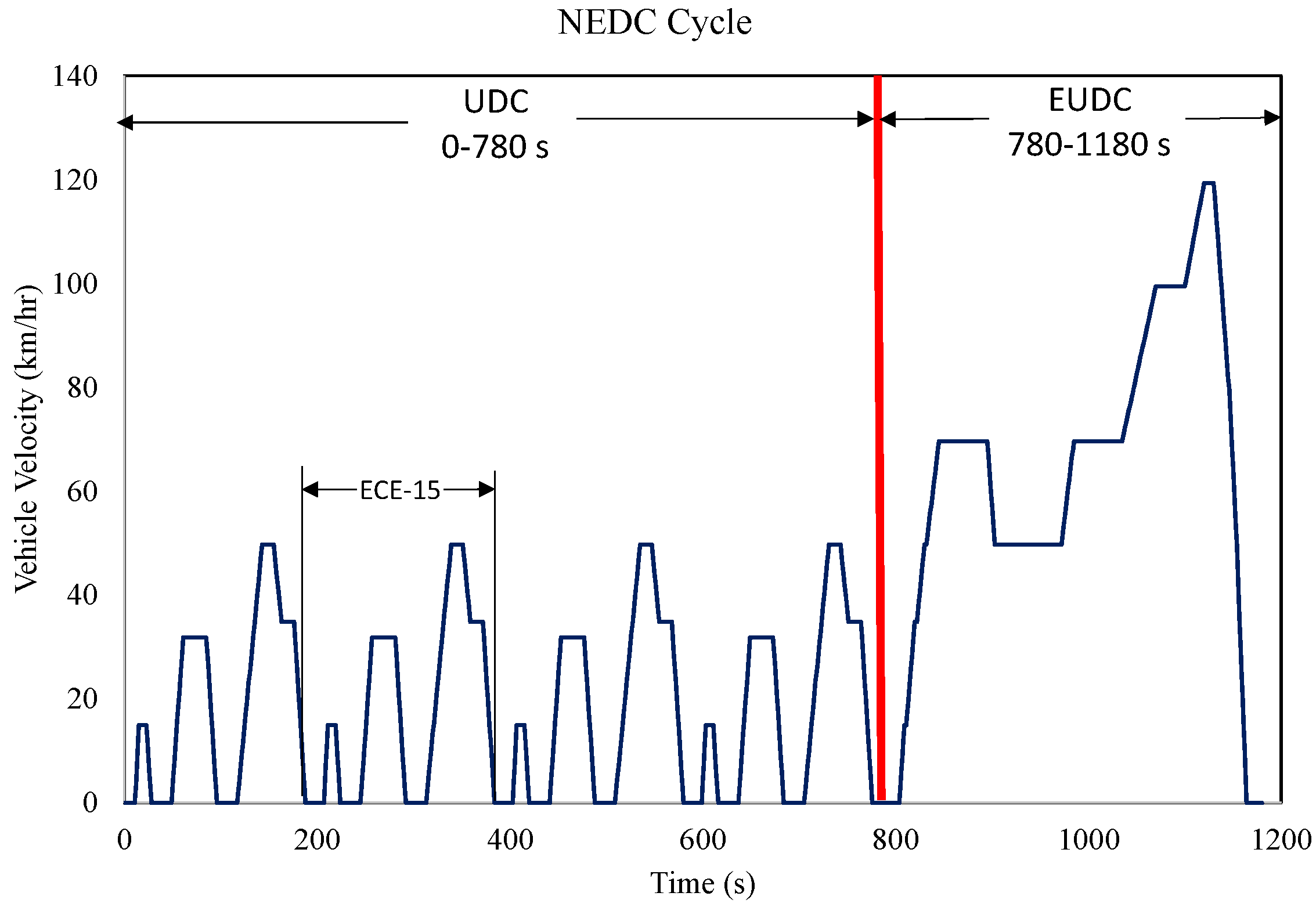
The entire simulation analysis began from the driving cycles based on the NEDC (Figure 1) for standardized testing procedures to provide instantaneous driving forces required to overcome the aerodynamic, rolling, grade, and inertia resistances. The entire driving cycle (total time, 1180 s) including urban driving cycles (UDCs) and extra-urban driving cycles (EUDCs). The first 780 s was the UDC (maximum speed 50 km/h), and the next 400 s was the EUDC (maximum speed 120 km/h).
Figure 1.
NEDC driving cycle.

2.2. Vehicle Dynamic Model
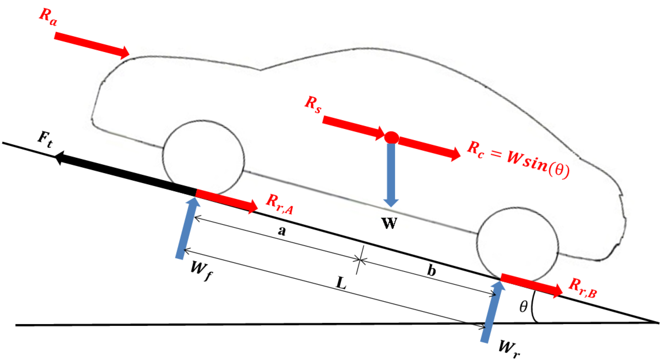
Figure 2 (red arrows) shows the vehicle driving resistances, including the rolling, aerodynamic, grade, and acceleration resistances. The vehicle driving forces are calculated through the dynamic vehicle model by using the following equations:
where Ft is the tractive effort; Rr is the rolling resistance; μr is the rolling resistance coefficient, W is the vehicle weight; Ra is the aerodynamic dragging force; CD is the aerodynamic dragging coefficient; v is vehicle speed; vw is wind speed; Rc is the grade resistance; We is the equilibrium weight of rotational part; a is vehicle acceleration; and Rs is the inertia force. The grade was set to 0 in all fuel economy simulations.
Figure 2.
Vehicle dynamic analysis.

2.3. Engine Model
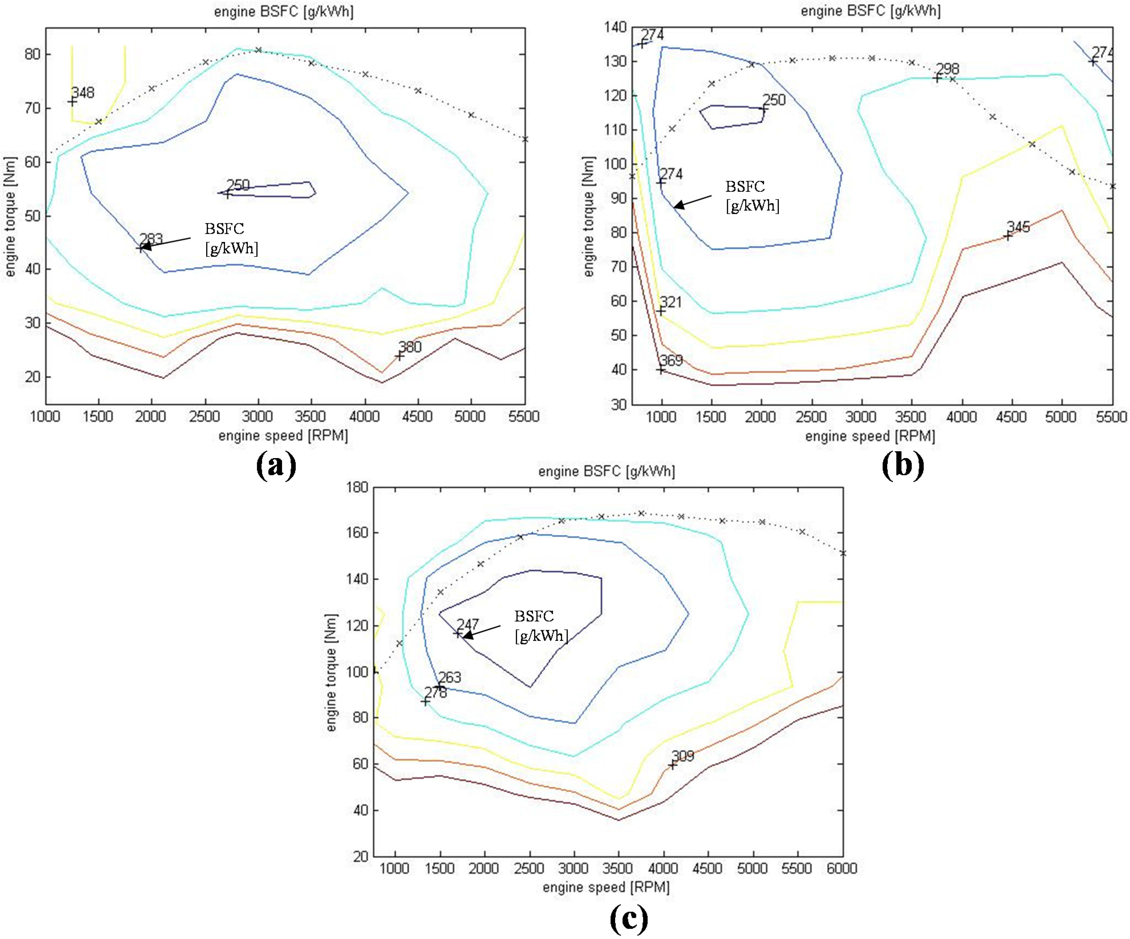
The engine model in this study was a steady state engine model. Vehicle fuel consumption is related to the engine operating conditions. Therefore, the speed and time required for the driving cycles is converted to engine speed and torque. The look-up table method was applied to obtain the brake specific fuel consumptions (BSFC) for the known engine speeds and engine torques and subsequently calculate the vehicle fuel consumptions. Engine specifications for series, parallel, and conventional vehicles were designed by dividing gasoline engines into three displacement volumes of 1.0, 1.3, and 1.8 L, which generate maximal powers of 41, 63, and 95 kW, respectively. Figure 3 presents BSFC diagrams. The three engines were designed to be compatible with each basic configuration. The conventional manual transmission vehicle (MT) is equipped with a 1.8 L engine. The parallel hybrid systems, PHEV and PHHV, use a 1.3 L engine. Since they have an electric motor that assists driving power, their engine power can be lower than that of the MT vehicle. The series hybrid vehicles, which are driven by motors, use a 1.0 L engine. The engine is used to charge the battery. The average tractive power through the driving cycle is much lower than the peak power, therefore, the engine for series hybrid vehicles can be much smaller. The engine data in Figure 3 were retrieved from the ADVISOR 2003 database [19].
Figure 3.
The BSFC contour diagrams for (a) 41, (b) 63, and (c) 95 kW gasoline engines.

2.4. Power Component Model
2.4.1. Electric Motor Model
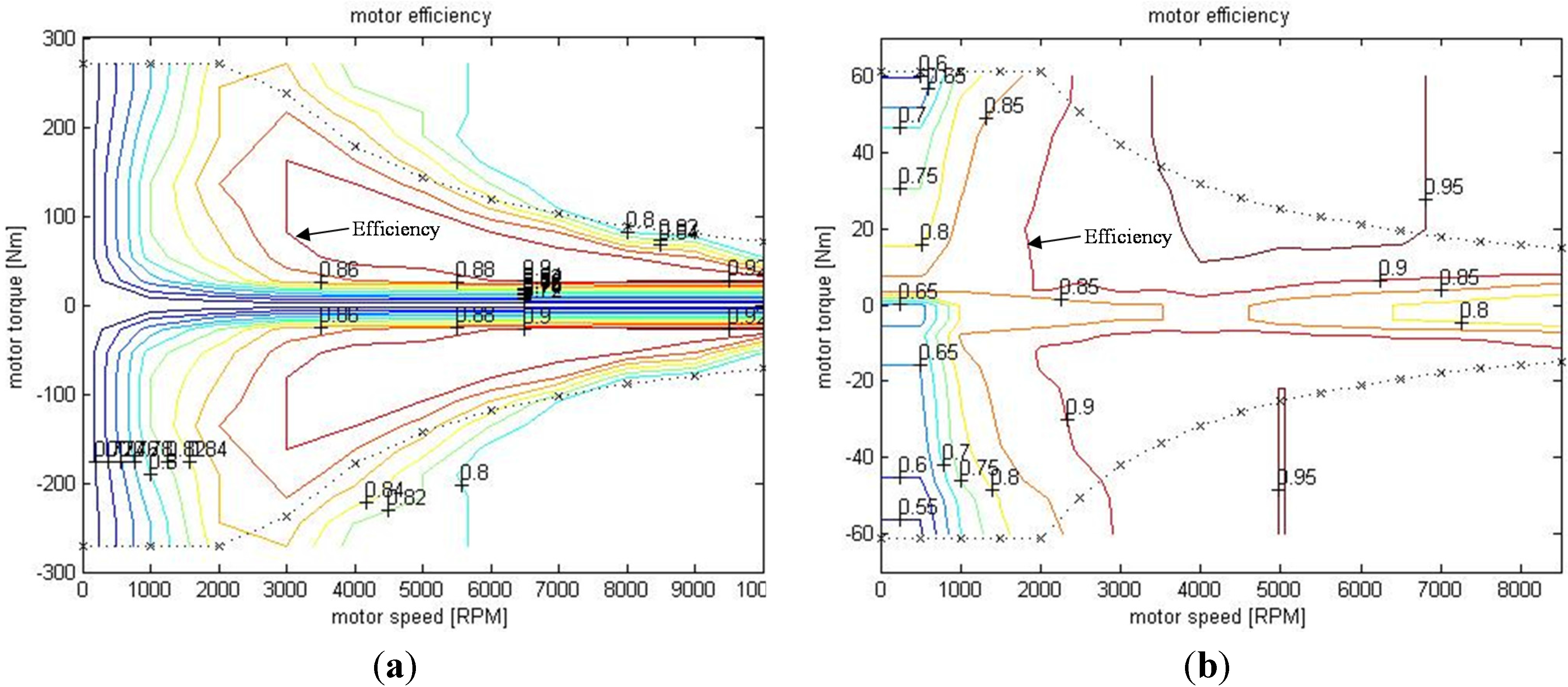
The electric motors were permanent magnet motors with outputs of 75 and 10 kW, which were used in the series and parallel systems, respectively. This direct current motor model features high torque at low operating speed. The powers required of the motors were calculated from the known required motor torques and motor speeds by using motor efficiency curves (Figure 4). The motor data in Figure 4 were retrieved from the ADVISOR 2003 database [19].
Figure 4.
Efficiency contour diagrams for the (a) 75 and (b) 10 kW electric motors.

2.4.2. Generator Model
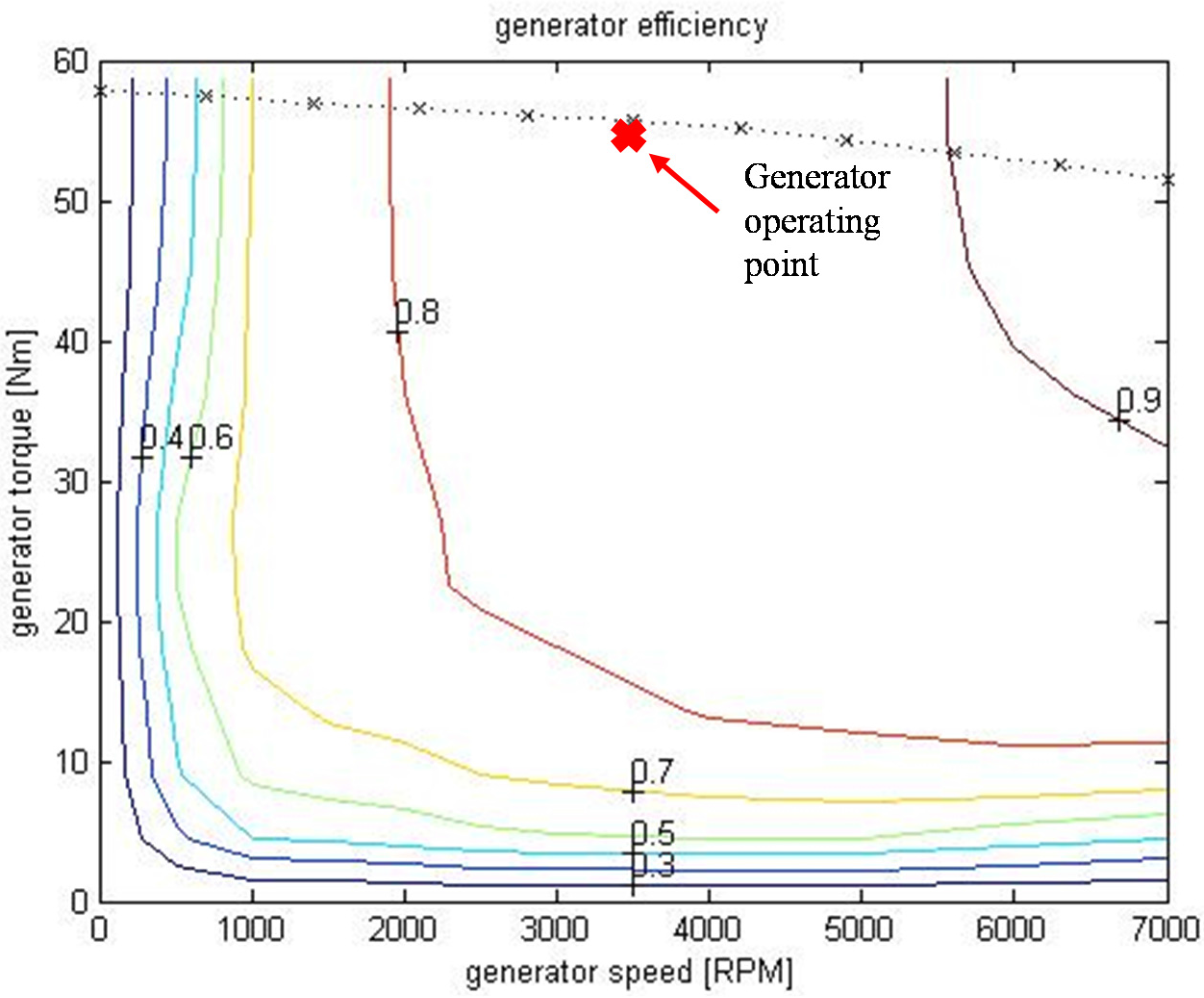
The generator model was used in only the SHEV system. In this model, a 32 kW permanent magnet generator is attached to a 1.0 L gasoline engine. The engine and generator are mainly controlled in a high-efficiency region during operation. The 1.0 L engine has high efficiency region around 3000 to 3500 rpm. The motor efficiency is also high (84% efficiency) in this region. Figure 5 shows the operating point. Therefore, the engine speed and engine torque were maintained at 3500 rpm and 55 Nm, respectively, to obtain the optimal fuel economy. Figure 5 shows the generator efficiency contour diagram. The data is retrieved from the ADVISOR 2003 database [19].
Figure 5.
Efficiency contour diagram for the 32-kW generator.

2.4.3. Hydraulic Motor and Hydraulic Pump Models
In hydraulic plunger motor–pumps, plungers reciprocate in limited volumes, vacuuming low-pressure hydraulic oil into the plunger chamber and displacing high-pressure hydraulic oil outside the chamber through plunger compression. During this process, displacements can be regulated from pressure and flow rate variations by adjusting axial (clinoaxis plunger) or swashplate (swashplate plunger) angles, subsequently changing torsional moment and rotational speed relationships. The total efficiency of the hydraulic motor–pump is the product of volumetric and mechanical efficiencies. Operating variables such as pressure difference and volumetric flow rate, hydraulic motor–pump parameters (volumetric displacement), and fluid parameters (fluid viscosity coefficient, density, and bulk modulus) typically influence efficiency. The efficiency of the hydraulic pump and motor varies according to the operating conditions such as pressure and volumetric flow rate [17]. The majority of the pump efficiency map, at a fixed flow rate, is populated with efficiency above 80%. Therefore, an overall efficiency of 80% was used for simulation. The hydraulic motor–pump-related equations are as follows:
The hydraulic motor/pump volumetric fluid flow rate is:
The hydraulic motor/pump shaft torque is:
The hydraulic motor/pump shaft power is:
where QPM is volumetric fluid flow rate; xPM is the fraction of volume displacement; DPM is the maximum volumetric displacement; ωPM is the shaft angular velocity; ∆PPM is the pressure difference between the hydraulic motor/pump outlet and the inlet; ηvPM is volumetric efficiency; ηtPM is mechanical efficiency; and Z is mode factor (+1 for pumping mode, −1 for motor mode).
2.5. Energy Storage Component Model
2.5.1. Lithium-Ion Battery Model
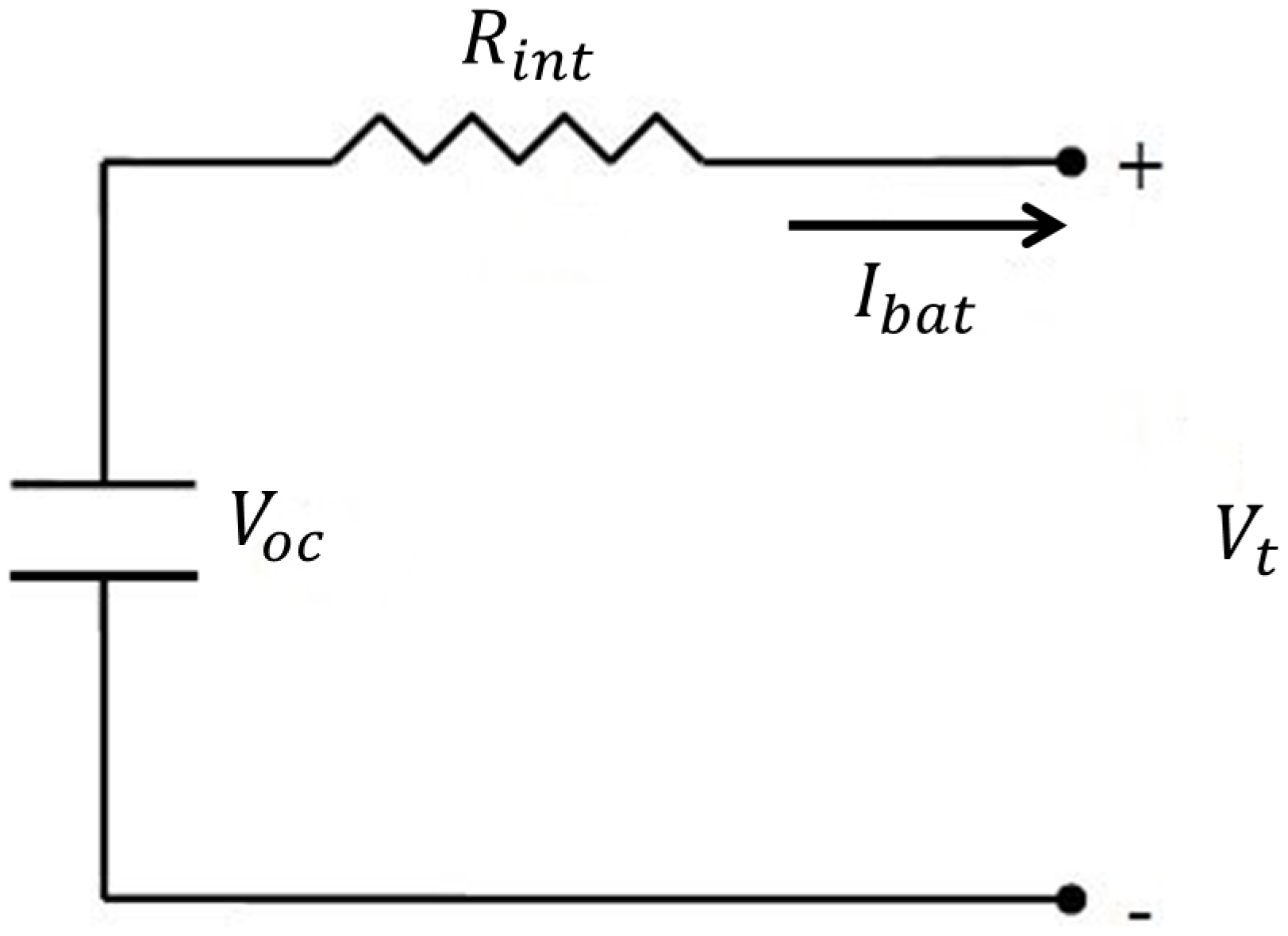
Lithium-ion batteries were adopted in this study. The total electric energy varied among PHEVs, SHEVs, and EVs, yielding 1, 2.5, and 25 kWh outputs, respectively. The battery model [20] can be established according to the simple resistor–capacitor circuit shown in Figure 6. The relevant equation is:
where Voc is the open circuit voltage of battery; Rint is the internal resistance of the battery; Vt is the battery terminal voltage; and Ibat is the battery output current.
Figure 6.
Resistor–capacitor circuit diagram for battery mode.

After measuring terminal voltages and currents, the following equation is used to obtain the battery power outputs (Pbat):
Furthermore, the following equation can be obtained by substituting Equation (9) into Equation (10):
Typically, battery SOCs are expressed using the battery capacity unit of amp-hour (Ah). Since SOCs vary by charge–discharge current, the following equation is used to obtain battery SOCs:
where SOCint is the initial SOC.
2.5.2. Accumulator Model
The energy that the accumulator requires from regenerative braking was calculated using the method proposed in [21]. The equation Ek = 1/2 mv2 was used to determine the energy of the accumulator. Assuming regenerative braking commences at v = 60 km/h, 209 kJ of energy can be recycled during each regenerative braking event. Therefore, accumulator volume was set to 18 L, and working pressure was set to 172 to 344 bar. The accumulator model can be established according to the polytropic process of the laws of thermodynamics. The variation process of the gaseous state must be considered to investigate the gaseous pressures and volumes because the accumulator is operated frequently in the HHV. Therefore, the gaseous state changes were considered to be an adiabatic process (rapid changes; n = 1.4) in this study. Temperature variations were not considered. During actual gaseous expansion and compression, the pressure and volume relationship is:
Moving boundary work:
Oil displacements:
where P0 is the initial enclosed gas pressure of accumulator; P1 is the maximum actuation pressure; P2 is the minimum actuation pressure; V0 is the accumulator volume; V1 is the volume with pressure P1; an V2 is the volume with pressure P2; and Vf is the volume of discharge oil from the accumulator.
Accumulator SOCs are typically expressed volumetrically because SOCs vary with volumetric flow rates. Therefore, the following equation can be used to obtain the accumulator SOC:
2.6. Manual Transmission Vehicle
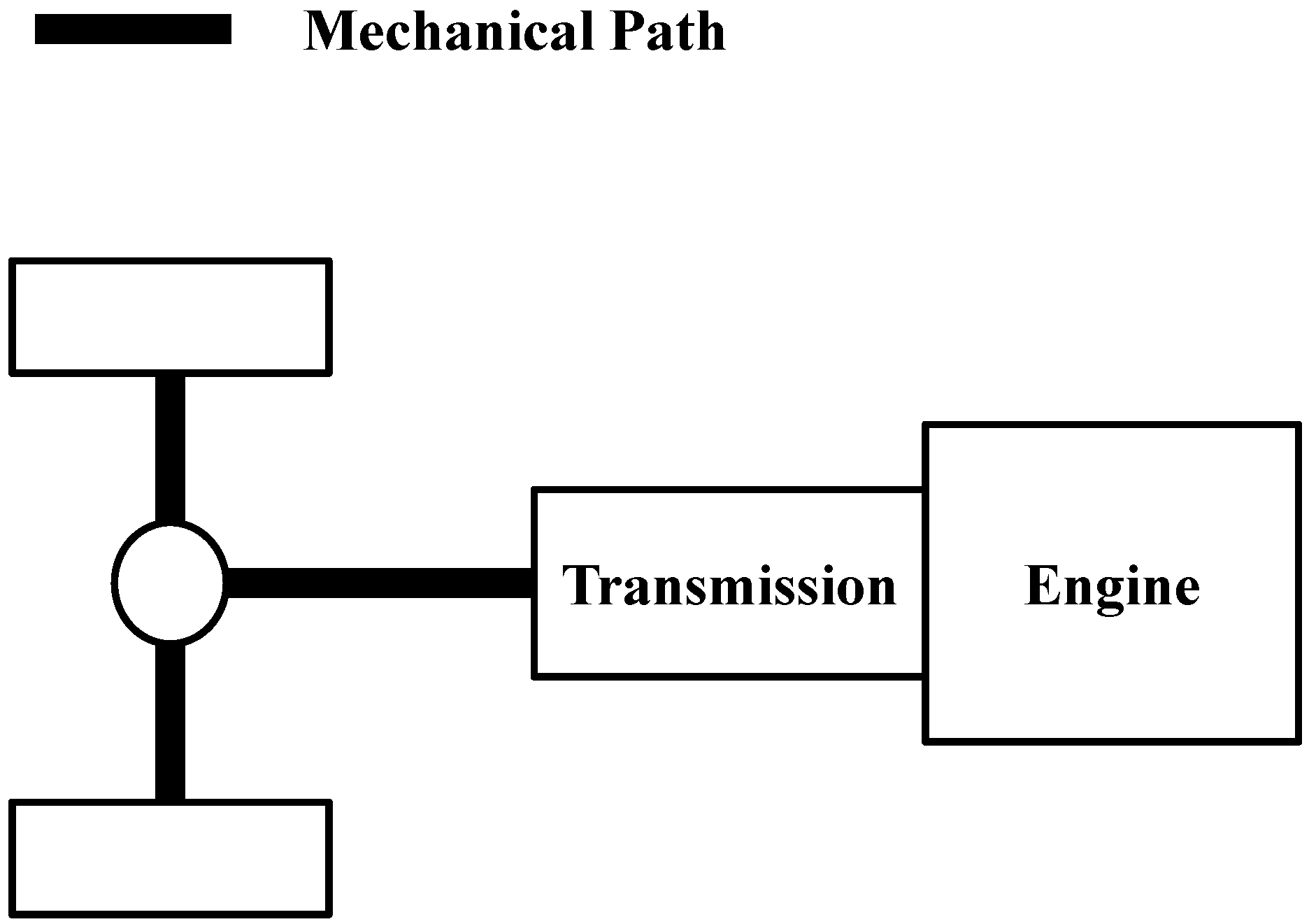
Figure 7 shows the conventional powertrain system model which comprised the subsystems of driving cycle, vehicle dynamic, transmission, and engine models. In the simulations, gearshifts were operated according to vehicle speeds and were assumed to be smooth and free from clutch slippage.
Figure 7.
Structural diagram of the manual transmission vehicle.

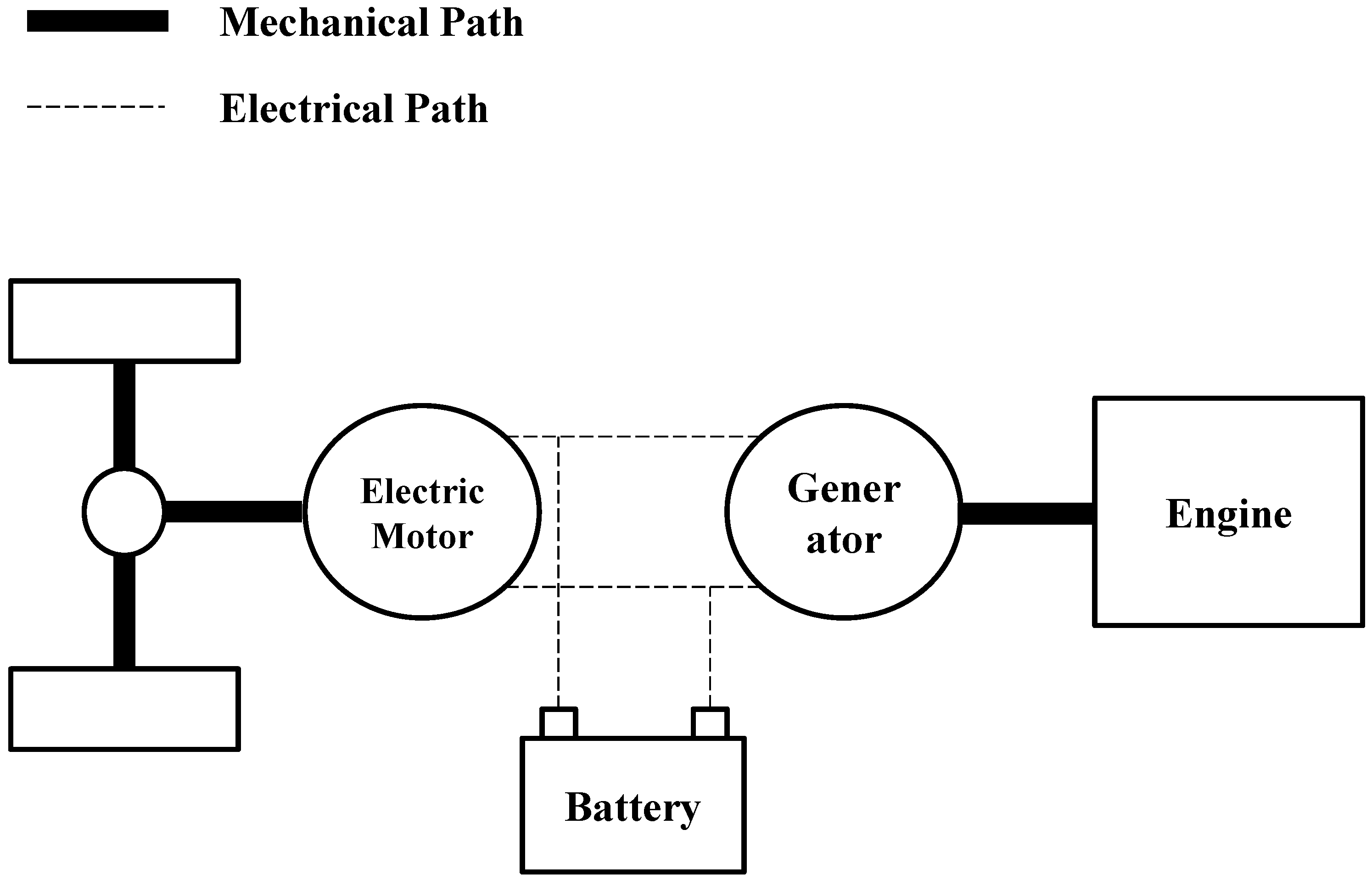
2.7. Series Hybrid Electric Vehicle
Figure 8 shows the SHEV powertrain system which comprised the driving cycle, vehicle dynamic, transmission system, power components (electric motor and generator), energy storage component (lithium-ion batteries), and engine model subsystems. In the simulations, the ON–OFF states of the engine were used to maintain the state-of-charge (SOC) of the lithium-ion batteries within a range of 0.35–0.65. The SOC range is designed to maintain the system in a high efficiency state, considering the combined efficiencies of both charging and discharging. The charging efficiency is high when SOC is low whereas the discharging efficiency is high when SOC is high [22]. This study chose the middle 30% of SOC, 0.35 to 0.65. The control procedures involved inspecting the engine status, determining the SOC, and determining whether the engine must be switched on to charge the lithium-ion batteries.
Figure 8.
Structural diagram of the SHEV.

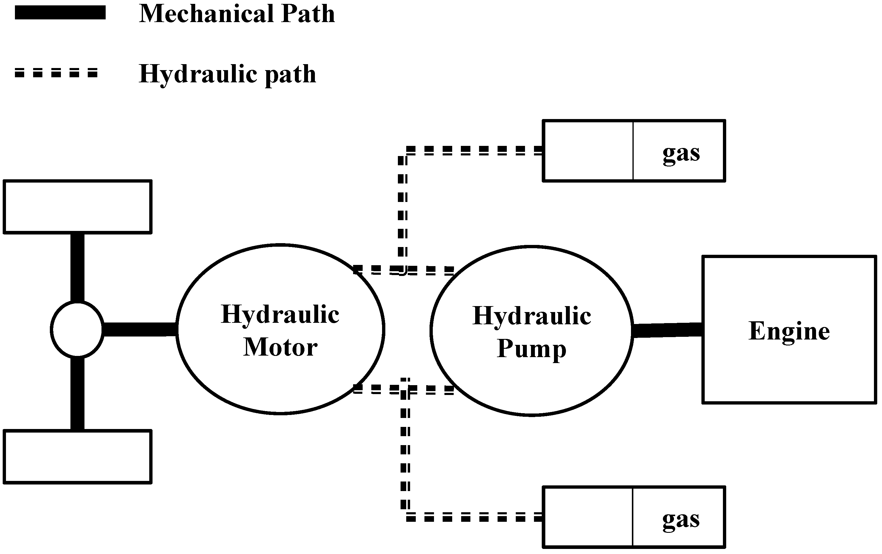
2.8. Series Hydraulic Hybrid Vehicle
Figure 9 shows the SHHV system model which comprised the driving cycle, vehicle dynamic, transmission system, power component (hydraulic motor and hydraulic pump), energy storage component (accumulator), and engine model subsystems. Regarding simulation controls, the ON–OFF states of the engine were used to control the SOC of the accumulator within the range of 0–1. The detailed control procedures were identical to those of the SHEV. The primary difference was that the accumulator had a larger SOC range than that of the lithium-ion batteries.
Figure 9.
Structural diagram of the SHHV.

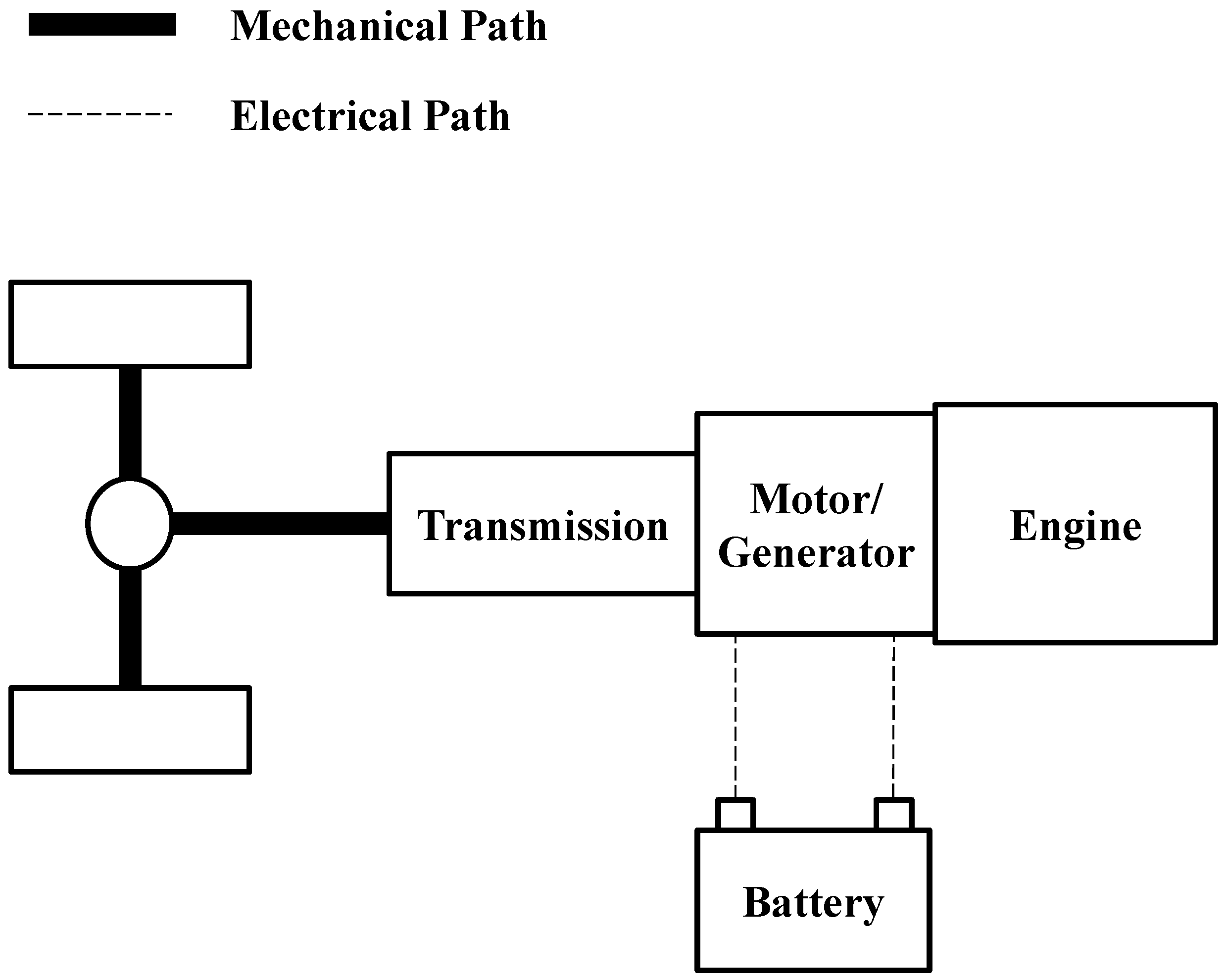
2.9. Parallel Hybrid Electric Vehicle
Figure 10 shows the PHEV system model which comprised the driving cycle, vehicle dynamics, transmission system, power component (electric motor), energy storage component (lithium-ion batteries), and engine model subsystems. Additionally, the simulation controls comprised pure electric (Mode A), pure engine (Mode B), hybrid (Mode C), engine charging (Mode D), and regenerative braking (Mode E) modes. In simulation, engine and electric motor torques were distributed according to specific road conditions (deciding among Modes A, B, and C) first. Then, the engine statuses were inspected to decide between the upper and lower SOC thresholds. The system proceeds to (engine) charging mode when battery SOC is below the set threshold; otherwise, the system proceeds according to the operating mode selected in the first step. The SOC operating range is maintained between 0.35 and 0.65.
Figure 10.
Structural diagram of the PHEV.

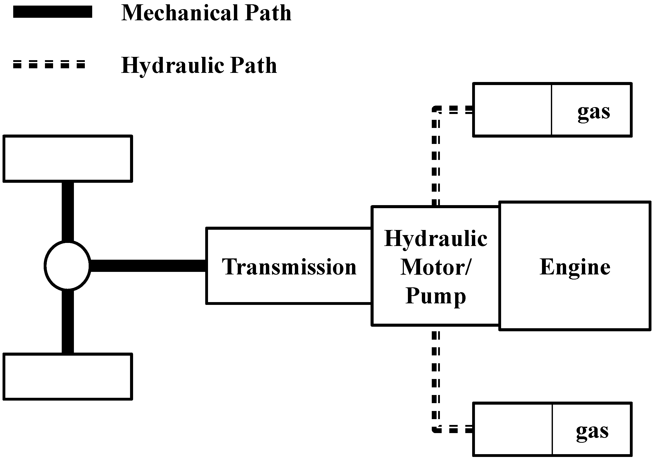
2.10. Parallel Hydraulic Hybrid Vehicle
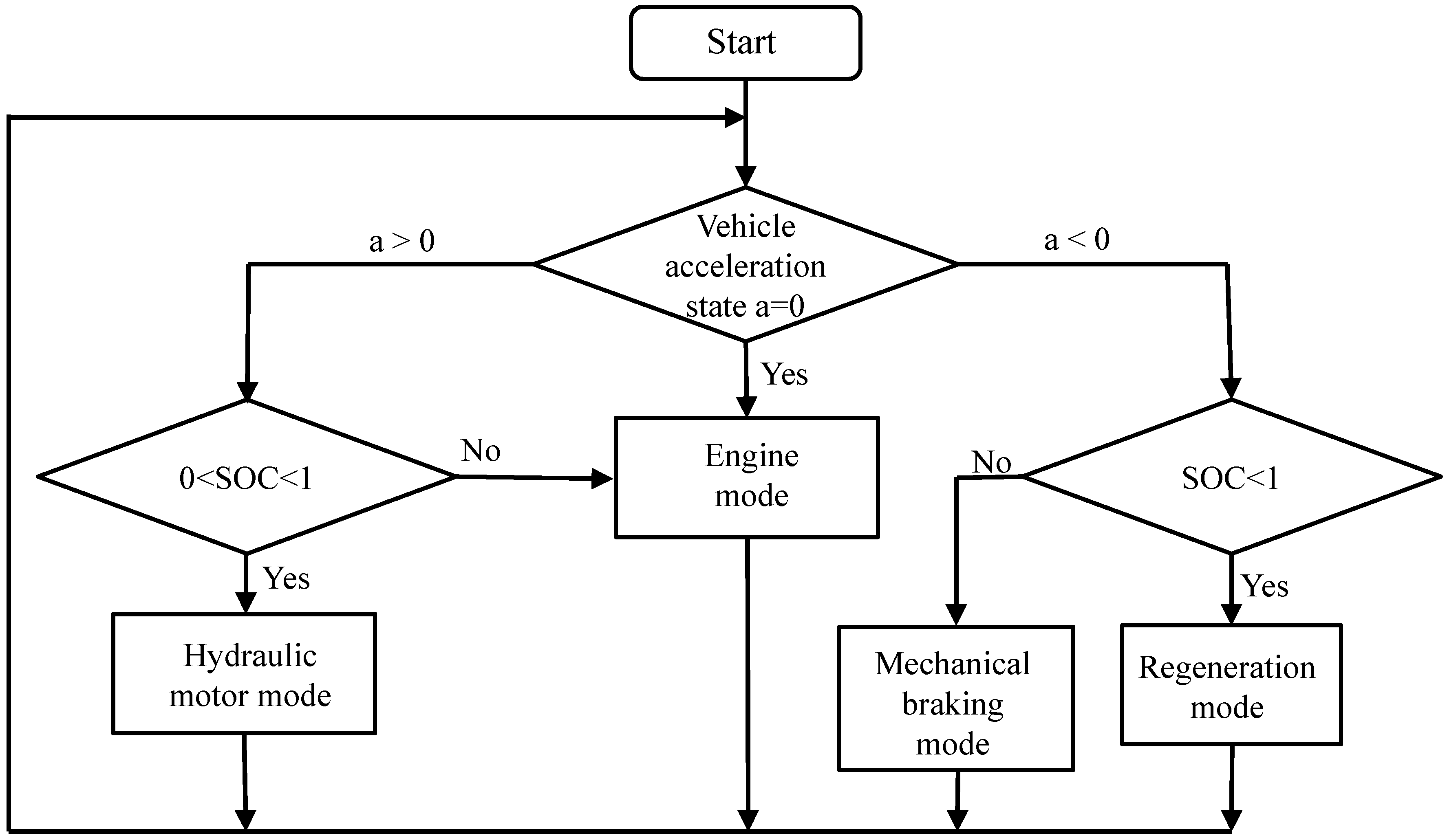
Figure 11 shows the PHHV system which comprised the driving cycle, vehicle dynamic, transmission system, power component (hydraulic motor), energy storage component (accumulator), and engine model subsystems. The start–stop method was applied to improve fuel consumption during vehicle starting and stopping [23]. The hydraulic motor and accumulator generated power for acceleration during vehicle startup. The vehicle was subsequently propelled by the engine as the accumulator depleted, and the engine was the only power source before the vehicle braking. The engine would be shut down when brake was applied. By preventing the engine from operating in an inefficient zone, this control strategy improves fuel economy. During vehicle braking, the hydraulic motor acts as a hydraulic pump that converts kinetic energy regenerated during braking into hydraulic energy and then recycles this energy to the accumulator for the next vehicle startup process. First, the state of vehicle acceleration was determined. When acceleration exceeds 0, the system proceeds to the second step to determine the SOC of the accumulator and to decide whether to operate with the hydraulic motor or in an engine mode. When acceleration equaled to 0, the system operates on engine mode, and when acceleration was less than 0, the system operates on regenerative braking mode, Figure 12.
Figure 11.
PHHV structural diagram.

Figure 12.
PHHV control flow chart.

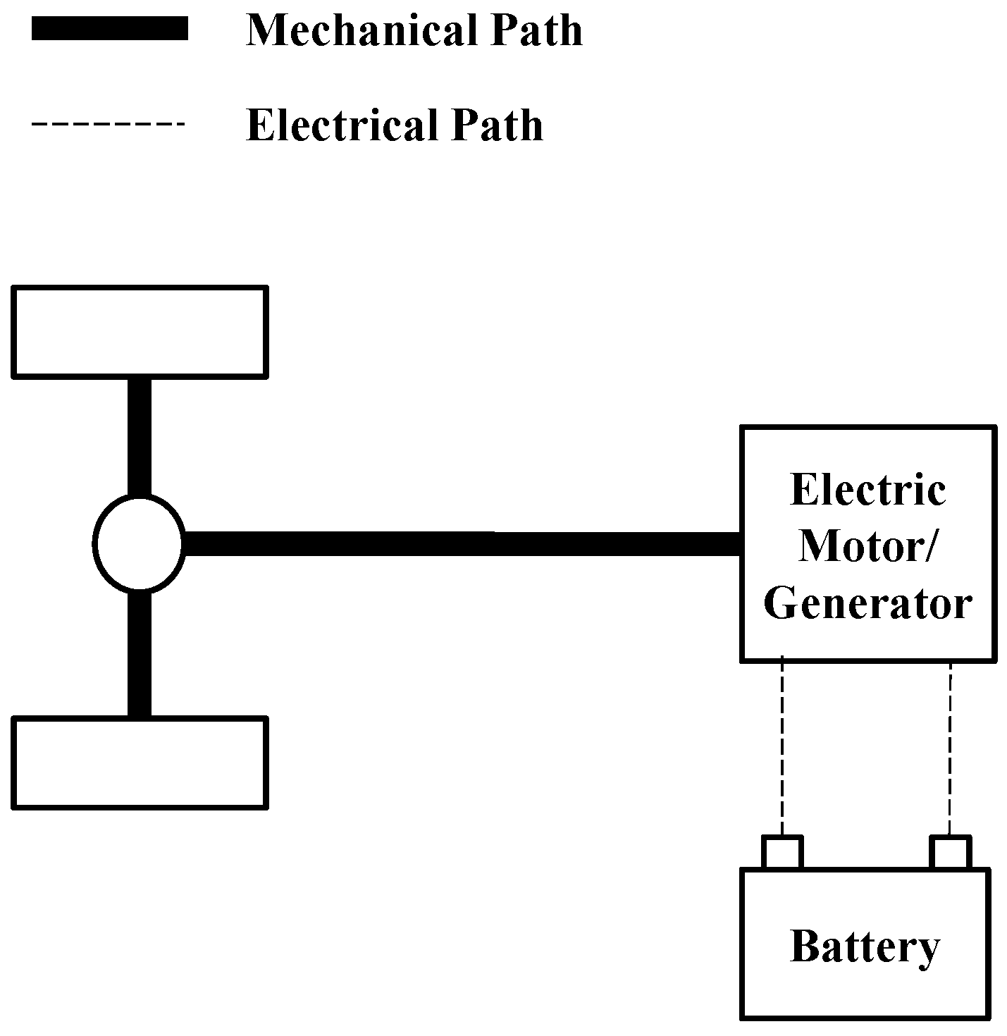
2.11. Electric Vehicle
Figure 13 shows EV system which comprised the driving cycle, vehicle dynamics, transmission system, power component model (electric motor), and energy storage component (lithium-ion batteries) model subsystems. The simulations placed restrictions on the maximum motor speed, maximum motor torque, and maximum power of the electric motor. Additionally, the maximum and minimum voltages were configured for the batteries to ensure normal operation.
Figure 13.
Structural diagram of the EV.

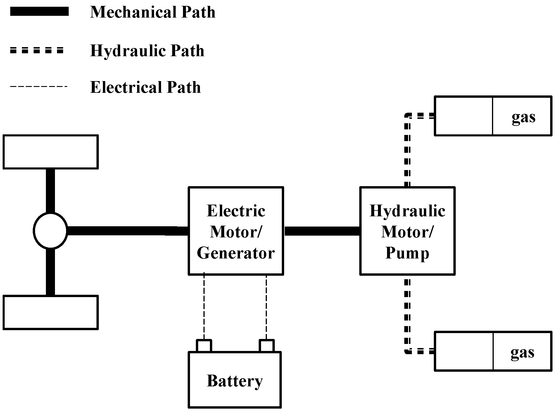
2.12. Hydraulic–Electric Hybrid Vehicle
HEHVs are primarily powered by electrical systems (electric motor and lithium-ion battery submodels) and assisted by hydraulic systems (hydraulic motor–pump and accumulator submodels). These systems reduce electrical energy consumption and extend the driving range (Figure 14).
Figure 14.
Structural diagram of the HEHV.

In simulations, the controls adopted the start–stop method identical to that applied in the PHHV system. In this study, the HEHV architecture was derived directly from that of the PHHV except the engine was replaced with an electric motor and battery. Therefore, the HEHV used the same control strategy as PHHV did, and the braking energy recycling was done by hydraulic motor instead of electric motor. The hydraulic motor is generally more efficient than the electric motor. In the HEHV, a hydraulic system is mainly used to recycle braking energy.
3. Simulation and Analysis
This section discusses the simulation results for the seven vehicle systems. Energy consumption was analyzed by simulating the NEDCs, and the performance of each component was compared. The required vehicle driving forces and powers for the NEDC were calculated first. Then, according to the performance analyzed for the manual transmission (MT) vehicles, the SHHV, PHHV, SHEV, PHEV, EV, and HEHV performance results were evaluated. Finally, the fuel economy of the SHHV, SHEV, PHHV, PHEV, EV, and HEHV systems was obtained.
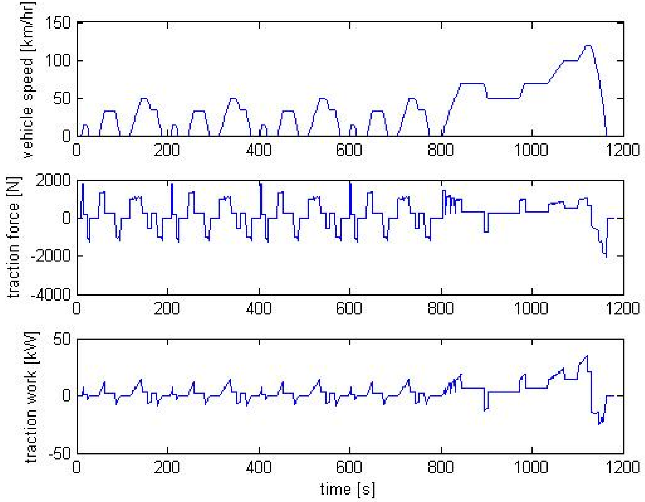
3.1. Driving Force and Power Required for the Driving Cycles
Regardless of vehicle type, specifications must be consistent in subsequent performance comparisons. Table 2 shows the common vehicle specifications. For hybrid vehicles, the fuel economy is less sensitive to its vehicle mass since part of the kinematic energy used to accelerate the vehicle can be recovered by regenerative braking. Moreover, the study focused on the fuel efficiency of different powertrain configurations. To minimize the effects of different component masses, this study tentatively disregarded the mass differences of the vehicles in order to compare the actual functional contribution of different powertrain configurations. During simulations, the required wheel driving force and power must be calculated using the driving cycle model (Figure 15). For example, the first, second, and third diagrams show the vehicle speeds, wheel driving force, and work required for the vehicles. The diagrams indicate that the maximal vehicle speed, wheel driving force, and power were 120 km/h, 1787 N, and 35 kW, respectively. Therefore, the power from the engine and electric motor in the series, parallel, and conventional vehicle systems should satisfy these conditions.
| Parameter | Symbol | Value | Unit |
|---|---|---|---|
| Vehicle mass | m | 1500 | kg |
| Frontal projected area | 2.26 | ||
| Air resistance coefficient | 0.28 | — | |
| Rolling resistance coefficient | 0.008 | — | |
| Wheel radius | r | 0.315 | m |
| Air density | 1.225 | ||
| Fuel density | 0.74 | ||
| Gravitational acceleration | g | 9.81 |
Figure 15.
Vehicle speed, wheel driving force, and power.

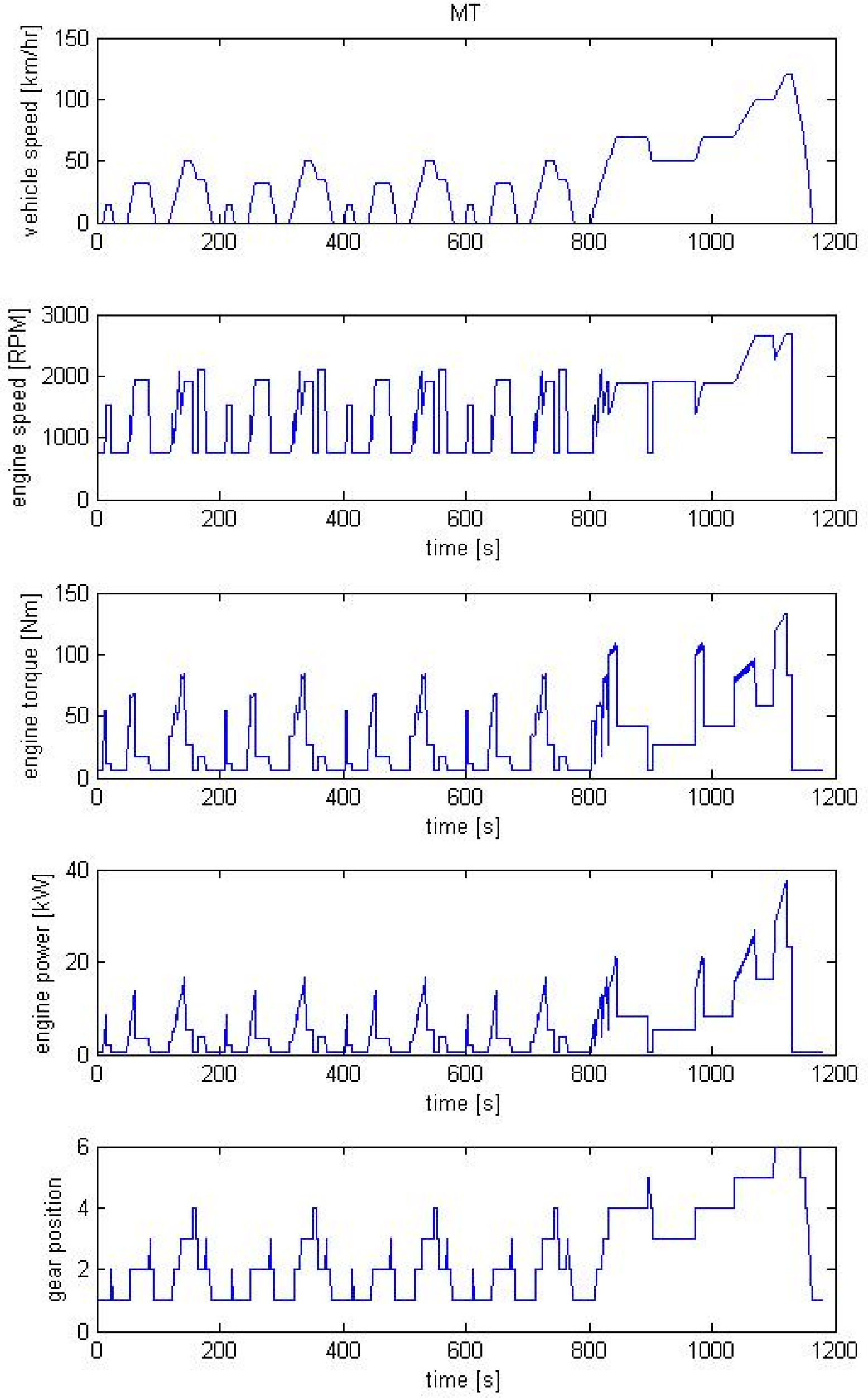
3.2. Performance Analysis of Conventional Manual Transmission Vehicles
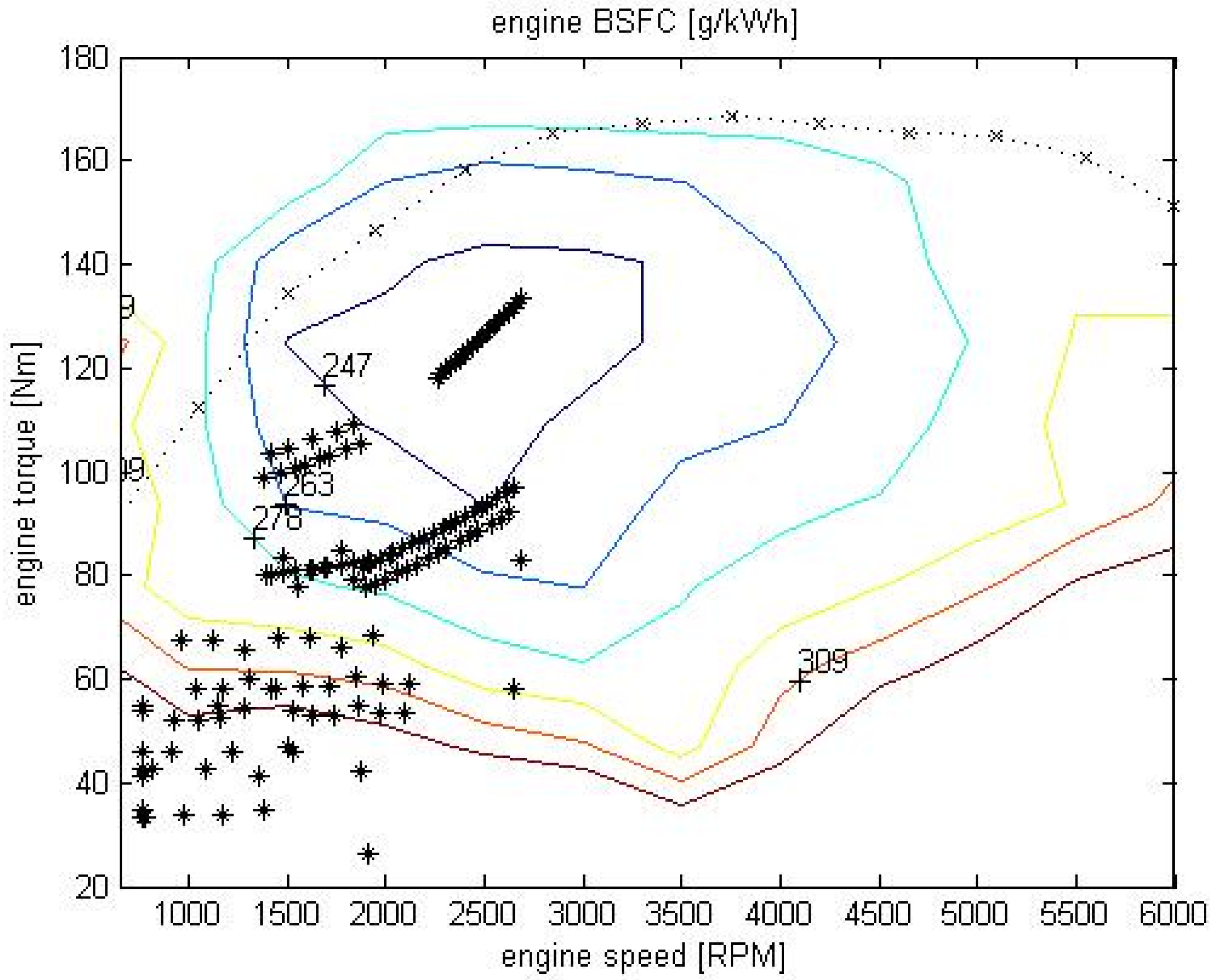
The performance of the MT vehicle was analyzed to facilitate comparison with the HEV and HHV. A model was established according to the specifications of a Toyota Camry with manual transmission and 1.8L gasoline engine. Figure 16 shows the engine operating conditions of an MT vehicle during NEDC. This figure presents, in descending order, the vehicle speed, engine speed, engine torsional moment, engine power, and gearshift conditions. These performance comparison results show that the NEDC reached a constant cruising speed after three stages of acceleration. To overcome these acceleration (including air and rolling) resistances, the engines must generate 8.6, 13.8, and 16.6 kW of power. Additionally, the maximal vehicle speed, engine speed, engine torque, and power during the entire driving cycle were 120 km/h (sixth gear), 2700 rpm, 135 Nm, and 37.5 kW, respectively. Figure 17 shows the engine operating conditions of the MT vehicle during the NEDC, which indicates that optimal fuel consumption (within 247 g/kWh) was obtained at high operating speed. During intermediate and low speed operations, fuel consumption ranged from 247 to 278 g/kWh and from 278 to 323 g/kWh, respectively. To evaluate the accuracy of simulation models, the Camry 2.0E fuel economy data was applied for the comparison between labeled fuel economy data and the MT simulation data. The fuel economies are presented in Table 3. During UDC and EUDC, the fuel economies were 8.88 and 6.59 L/100km, respectively, and average fuel consumption was 7.42 L/100km. The fuel economy of the MT vehicle during the UDC was 23.18% higher than that of Toyota Camry 2.0E. During the EUDC, the fuel economies of these two types of vehicle differed by 1.05%. Regarding average fuel consumption, the two vehicles differed by 12.08% in fuel economy, because the UDC varied more drastically within each driving cycle than EUDC did.
Figure 16.
Engine operating conditions of the MT vehicle.

Figure 17.
Engine operating points of the MT vehicle in the NEDC.

| Vehicle | Urban Fuel Consumption (L/100 km) | Extra-Urban Fuel Consumption (L/100 km) | Overall Fuel Consumption (L/100 km) |
|---|---|---|---|
| 2014 Toyota Camry 2.0E | 11.56 | 6.66 | 8.44 |
| MT | 8.88 | 6.59 | 7.42 |
| Difference (%) | −23.18 | −1.05 | −12.08 |
3.3. Performance Comparison between Series Hybrid Electric and Hydraulic Hybrid Vehicles
Figure 18a shows the performance diagrams for each component of the SHEV in the NEDC. The figure shows, in descending order, the vehicle speed, electric motor power, lithium-ion battery current, generator power, and lithium-ion battery SOC conditions. The data indicate that the engine started at 524 s and charged the battery until 733 s. This charging process was repeated at 1082 s, at which time the SOC was below 0.35. The engine started twice during this NEDC, when discharging-charging conditions (positive-negative variations) of the lithium-ion batteries were observed. Regarding the HHV, Figure 18b illustrates the performance diagrams for each component of the SHHV. The figure shows (from top to bottom) the vehicle speed, hydraulic motor power, accumulator pressure volumetric flow rate, pump power, and accumulator SOC. These simulations results revealed that the engine started ten times, which was eight more starts than in the SHEV, because the storage energy density of the accumulator was lower than that when lithium-ion batteries are used.
Figure 18.
Performance diagrams for each component in the (a) SHEV and (b) SHHV.

Regarding regenerative braking, the hydraulic motor (pump mode) could absorb high-power vehicle kinetic energy; thus, noticeable high power generation was observed during each vehicle deceleration (braking) session. Table 4 shows that, during UDC, fuel efficiency was 33.03% higher in the SHHV than in the SHEV.
| Vehicle Configuration | Urban Fuel Consumption (L/100 km) | Extra-Urban Fuel Consumption (L/100 km) | Average Fuel Consumption (L/100 km) |
|---|---|---|---|
| SHEV | 5.62 | 6.66 | 6.28 |
| SHHV | 3.77 | 5.57 | 4.91 |
| Difference (%) | −33.03 | −16.37 | −21.80 |
3.4. Performance Comparison between Parallel Hybrid Electric and Hydraulic Hybrid Vehicles
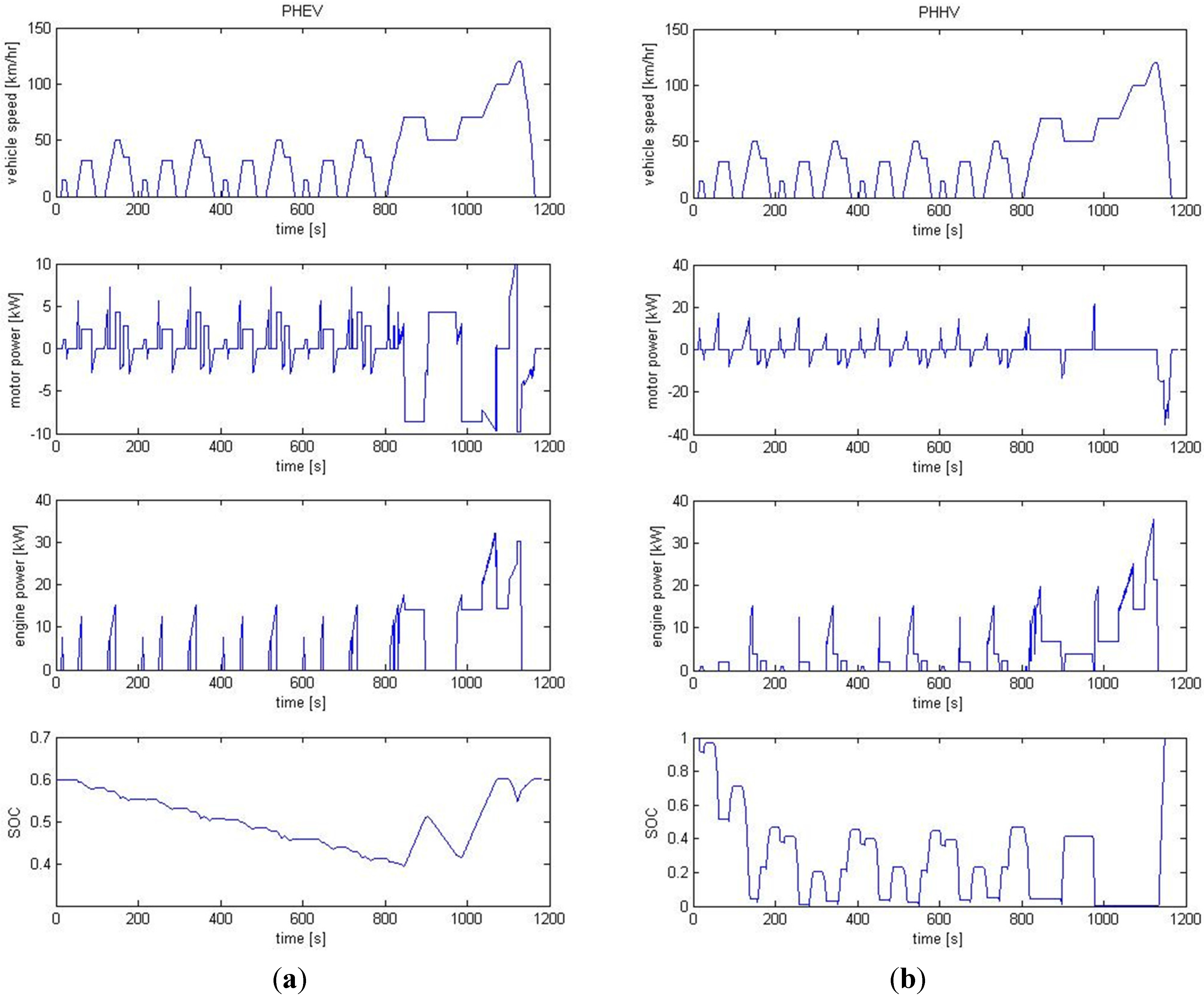
Figure 19a shows the performance diagrams for each component of the PHEV in the NEDC. The figure presents in descending order, the vehicle speed, electric motor power, engine power, and lithium-ion battery SOC order. The second and third diagrams show the coordination between the electric motor and engine. Figure 19b illustrates the performance diagrams for each component of the PHHV in the NEDC. In descending order, the figures show vehicle speed, hydraulic motor power, engine power, and accumulator SOC. These simulation results indicate that the hydraulic motor generated a substantially higher power compared with the electric motor during startup. Therefore, the control strategy used the hydraulic motor for startup and low-speed conditions and hydraulic pumps for energy recycling during deceleration (braking) sessions. Figure 20 illustrates the power distributions of engine and electric motor in pure electric motor, pure engine, engine charging, hybrid, and regenerative braking modes of the PHEV in the NEDC. In the default strategy, a torque of less than 40 Nm indicates a pure electric motor mode (Mode A), which can prevent engine operation in a region of low torque and low fuel efficiency. Between 40 and 85 Nm, the system operates in a pure engine mode (Mode B). Hybrid mode (Mode C) commences when the required torque exceeds 85 Nm, which is the region of optimal engine efficiency. During the engine charging mode (Mode D), the vehicle continues to operate and charge the batteries. Moreover, the engine can operate in the region of low fuel consumption. Figure 21 shows the engine operating point of the hydraulic assist system, which indicates that the engine generally operates in the high efficiency region. Finally, Table 5 shows the fuel economies of PHEV and PHHV. In the UDC, PHHV exhibited 6.32% higher fuel conservation compared with the PHEV. This difference occurred mainly because the control strategy for the PHHV prefers low-speed, startup, and regenerative braking conditions. In the EUDC, a reduced number of regenerative braking reflected 9.26% worse fuel economy in the PHHV compared with the PHEV.
Figure 19.
Performance diagrams for each component in the (a) PHEV and (b) PHHV.

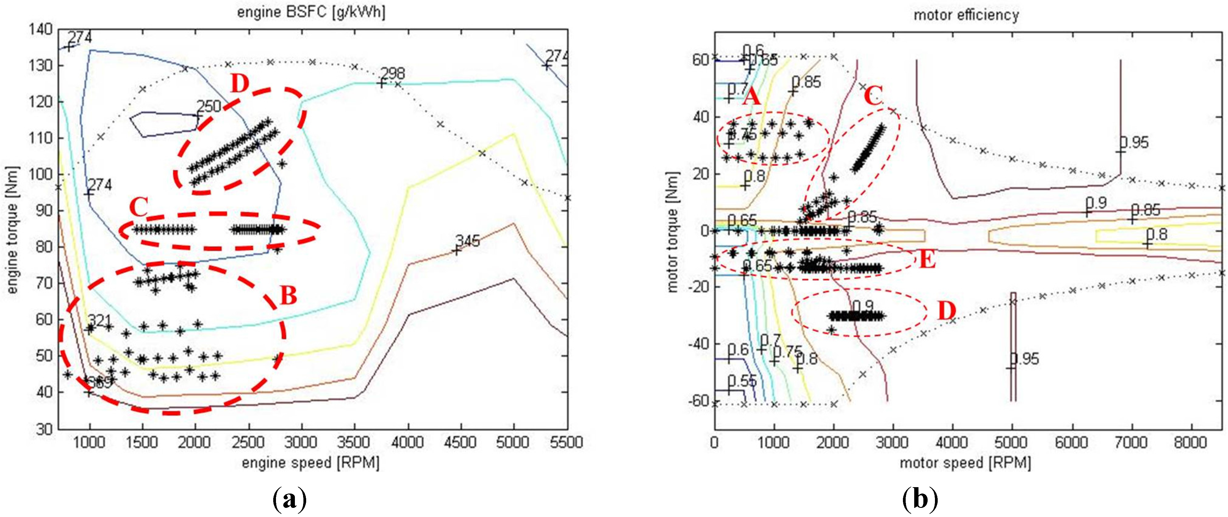
Figure 20.
PHEV operating points of the (a) engine and (b) electric motor.

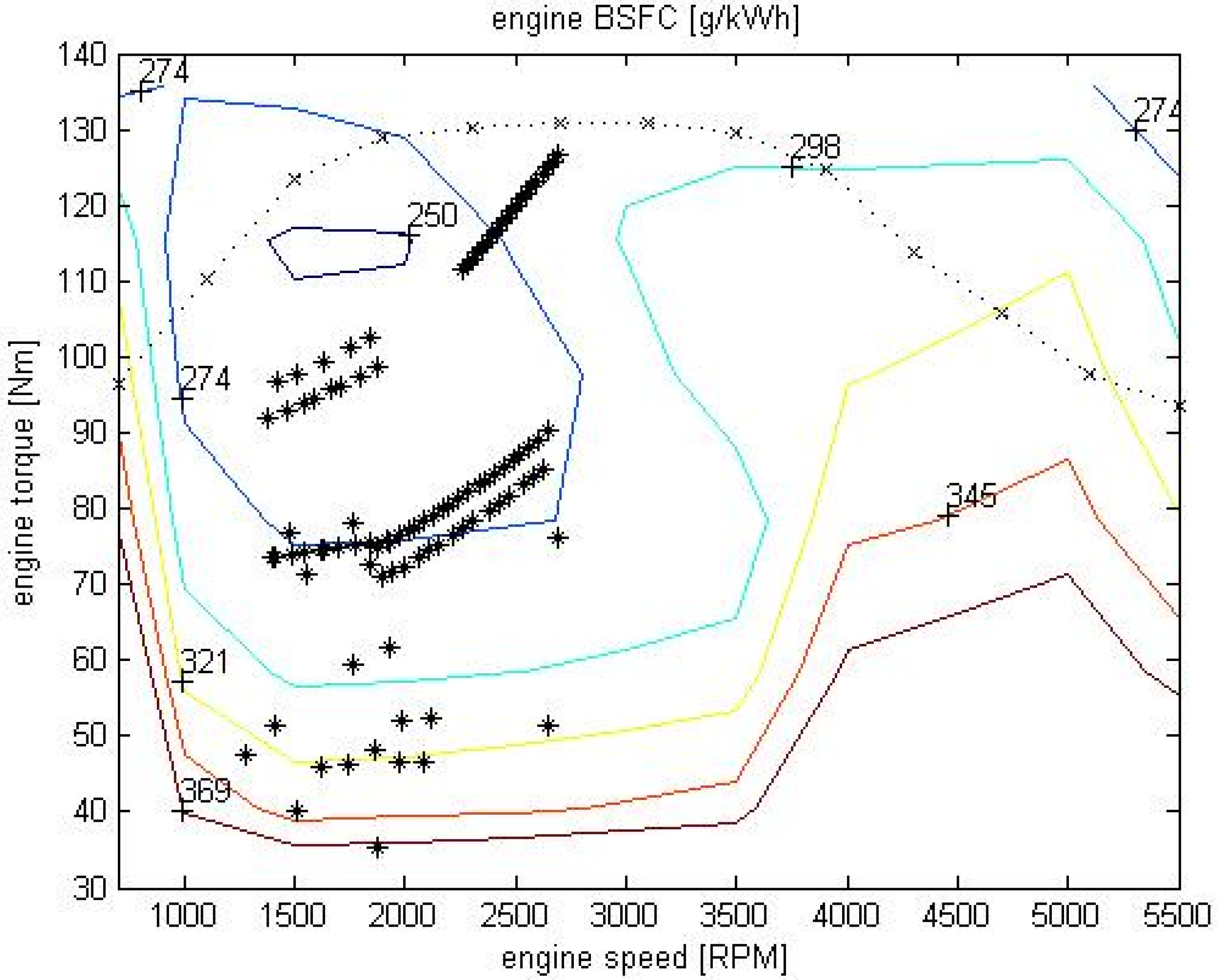
Figure 21.
PHHV engine operating points.

| Vehicle Configuration | Urban Fuel Consumption (L/100 km) | Extra-Urban Fuel Consumption (L/100 km) | Average Fuel Consumption (L/100 km) |
|---|---|---|---|
| PHEV | 4.41 | 4.68 | 4.58 |
| PHHV | 4.13 | 5.12 | 4.76 |
| Difference (%) | −6.32 | 9.26 | 3.80 |
3.5. Performance Comparison between Electric and Hydraulic–Electric Hybrid Vehicles
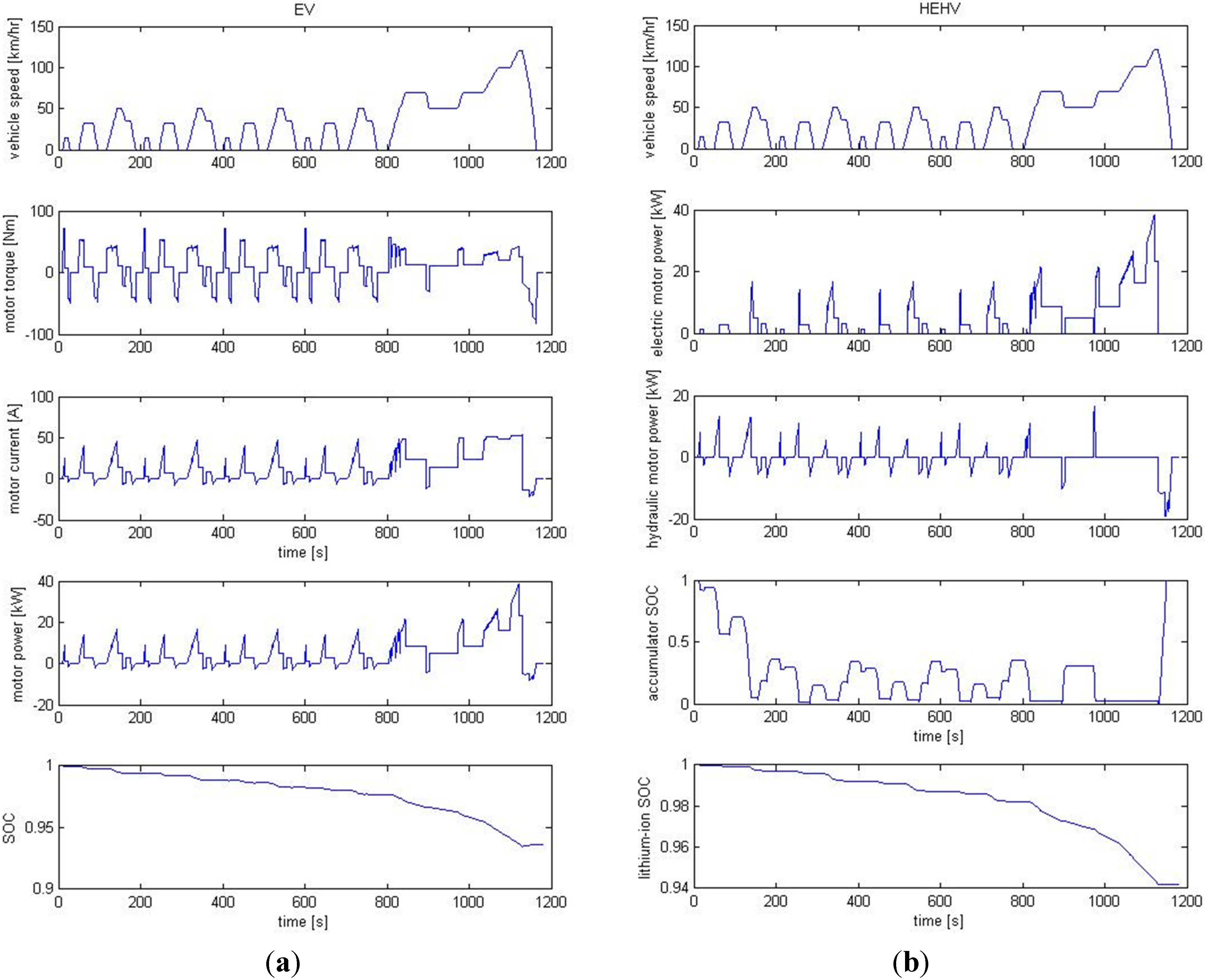
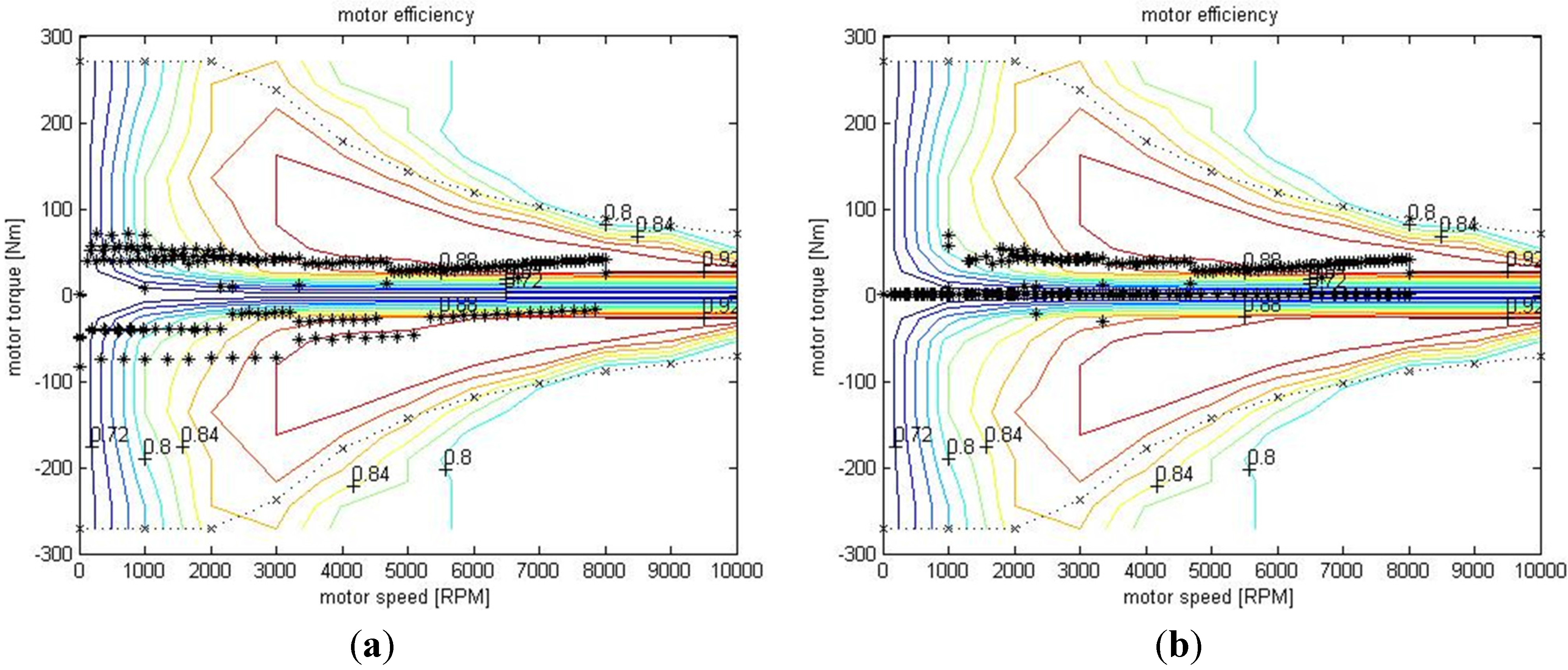
Figure 22a shows the performance diagrams for each component of the EV in the NEDC. In descending order, the figure presents the vehicle speed, electric motor torque, electric current, power, and lithium-ion battery SOC. Figure 22b illustrates the performance diagrams for each component of the HEHV in the NEDC. In descending order, the figure shows the vehicle speed, electric motor power, hydraulic motor power, lithium-ion battery SOC, and accumulator SOC. According to the electric motor operating points shown in Figure 23, the HEHV was driven by the hydraulic assist system in the low-speed region (electric motor in idling condition); therefore, the electric motor can be replaced by the hydraulic motor to power the vehicle during low speeds. In the high-speed region, the hydraulic assist system disengages. During regenerative braking, kinetic energy is recycled by using the hydraulic assist system (pump mode) instead of the electric motor. Table 6 indicates that, in the UDC, the HEHV consumed less energy than the EV did mainly because the hydraulic assist system prevented the electric motor from operating in the low-efficiency region (72% efficiency) at low speeds. Therefore, electricity consumption was decreased by 23.38%. In the EUDC, the energy consumption of the HEHV and EV did not substantially differ because the hydraulic assist system primarily operated during startup and stopping. Therefore, the hydraulic assist system was less frequently used in the EUDC than in the UDC, consequently conserving only 4.34% of electricity. Regarding total energy consumption, the HEHV provided 11.4% more electricity conservation compared with the EV.
Figure 22.
Performance diagrams for each component in the (a) EV and (b) HEHV.

Figure 23.
Electric motor operating points of the (a) EV and (b) HEHV.

| Vehicle Configuration | Urban Energy Consumption (MJ) | Extra-Urban Energy Consumption (MJ) | Total Energy Consumption (MJ) |
|---|---|---|---|
| EV | 2.079 | 3.528 | 5.607 |
| HEHV | 1.593 | 3.375 | 4.968 |
| Difference (%) | −23.38 | −4.34 | −11.40 |
Operating costs were converted to new Taiwan dollars per km (NT$/km) for a consistent comparison of all seven configurations of vehicles. According to the assumptions that the oil and electricity prices are NT$35/L and NT$5/kWh in Taiwan, Table 7 was obtained. The energy consumed per km was also included in Table 7.
| Items | Urban | Extra-Urban | Average | |||
|---|---|---|---|---|---|---|
| Metric | NT$/km | kJ/km | NT$/km | kJ/km | NT$/km | kJ/km |
| MT vehicle | 3.11 | 3073 | 2.31 | 2279 | 2.60 | 2568 |
| SHEV | 1.97 | 1946 | 2.33 | 2304 | 2.20 | 2174 |
| SHHV | 1.32 | 1303 | 1.95 | 1927 | 1.72 | 1700 |
| PHEV | 1.54 | 1526 | 1.64 | 1620 | 1.60 | 1586 |
| PHHV | 1.45 | 1430 | 1.79 | 1770 | 1.67 | 1646 |
| EV | 0.726 | 523 | 0.705 | 507 | 0.712 | 513 |
| HEHV | 0.556 | 401 | 0.674 | 485 | 0.631 | 455 |
3.6. Comparison of the Mass Effect on Energy Consumption
In all of the above simulations, vehicle mass was set to 1500 kg in order to focus on the energy efficiency of different powertrain systems. In this section, a 100 kg mass increment is added to the six derived powertrain systems to simulate the extra add-on masses from the energy storage medium, e.g., batteries and accumulators, and any energy transformation devices, e.g., motor/generators and pump/motors. Table 8 summarizes the analytical results for the effect of mass on energy consumption, which indicate that, with extra mass increment, HEHV consume relatively less energy.
| kJ/km | m = 1500 kg | m = 1600 kg | Diff. |
|---|---|---|---|
| SHEV | 2174 | 2244 | 70 |
| SHHV | 1700 | 1793 | 93 |
| PHEV | 1586 | 1630 | 44 |
| PHHV | 1646 | 1707 | 61 |
| EV | 513 | 532 | 19 |
| HEHV | 455 | 469 | 15 |
4. Conclusions
To effectively design environmentally friendly, energy efficient and cost beneficial vehicles, this research compares the energy consumption based on New European Driving Cycle using backward simulation in MATLAB/Simulink through various power component models, connection with energy storage component models, and combinations of series or parallel configurations. The study focuses on the energy efficiency comparison among different powertrain configurations. The setting for vehicle mass was similar in all simulation models to minimize the effects of different component masses and to clarify the actual functional contribution of each powertrain system. The operating efficiencies for each component were comprehensively compared. The fuel economy, power component, and energy storage component SOC of the HEV and HHV were obtained through the NEDC simulation. The conclusions of this study are as follows:
- (1)
- In the MT vehicle performance analysis, UDC and EUDC had fuel consumptions of 8.88 and 6.59 L/100 km (average, 7.42 L/100 km), respectively.
- (2)
- In the performance comparison between the SHEV and SHHV, SHHV conserved 33.03% more fuel than did the SHEV in the UDC. The improved efficiency is obtained by the hydraulic motor (pump mode), which has a higher capacity for absorbing the vehicle kinetic energy compared with the electric motor. Therefore, high power outputs by the hydraulic pump were clearly observed during each vehicle deceleration (braking) session.
- (3)
- In the performance comparison between the PHEV and PHHV, the PHHV conserved 6.32% more fuel compared with the PHEV. This is because the PHHV control strategy focused on low-speed, startup, and regenerative braking. In the EUDC, the PHHV had a 9.26% worse fuel economy compared with the PHEV because of the reduced number of regenerative braking sessions.
- (4)
- The performance comparison of the EV and HEHV revealed that the HEHV exhibited 23.38% higher electricity conservation compared with the EV in the UDC primarily because the hydraulic assist system prevented the electric motor from operating in the low-efficiency region (72%) during low-speed operations. In the EUDC, the HEHV conserved only 4.34% electricity. Regarding total energy consumption, the HEHV conserved 11.4% more electricity compared with the EV.
- (5)
- The experimental results revealed that, regardless of whether the UDC or EUDC was used, the HEHV had the best energy-conservation performance (average, NT$0.631/km). Table 9 shows that, for the MT vehicle used in this study, the HEHV presented a 75.7% improvement in economic savings.
| Configuration | Percentage Improvement (%) |
|---|---|
| MT vehicle used in this study | — (Baseline) |
| SHEV | 15.4 |
| SHHV | 33.8 |
| PHEV | 38.2 |
| PHHV | 35.9 |
| EV | 72.6 |
| HEHV | 75.7 |
Nomenclature
| CD | aerodynamic dragging coefficient |
| DPM | maximum volumetric displacement |
| EV | electric vehicle |
| Ft | tractive effort |
| HEHV | hydraulic-electric hybrid vehicle |
| Ibat | battery output current |
| PHEV | parallel hybrid electric vehicle |
| PHHV | parallel hydraulic hybrid vehicle |
| P0 | initial enclosed gas pressure of accumulator |
| P1 | maximum actuation pressure |
| P2 | minimum actuation pressure |
| QPM | volumetric fluid flow rate |
| Ra | aerodynamic dragging force |
| Rc | grade resistance |
| Rint | internal resistance of the battery |
| Rr | rolling resistance |
| Rs | inertia force |
| SHEV | series hybrid electric vehicle |
| SHHV | series hydraulic hybrid vehicle |
| V0 | accumulator volume |
| V1 | volume with pressure P1 |
| V2 | volume with pressure P2 |
| Vf | volume of discharge oil from the accumulator |
| Voc | open circuit voltage of battery |
| Vt | battery terminal voltage |
| W | vehicle weight |
| We | equilibrium weight of rotational part, |
| Z | mode factor (+1 for pumping mode, −1 for motor mode) |
| a | vehicle acceleration |
| m | vehicle mass |
| xPM | percentage of volume displacement |
| v | vehicle speed |
| vw | wind speed |
| ηvPM | volumetric efficiency |
| ηtPM | mechanical efficiency |
| μr | rolling resistance coefficient |
| ωPM | haft angular velocity |
| ∆PPM | pressure difference between the hydraulic motor/pump outlet and the inlet |
Acknowledgments
The author would like to thank the Ministry of Science and Technology of the Republic of China for financially supporting this research under Contract No. MOST 103-2221-E-027-024.
Conflicts of Interest
The author declares no conflict of interest.
References
- Doucette, R.T.; McCulloch, M.D. Modeling the prospects of plug-in hybrid electric vehicles to reduce CO2 emissions. Appl. Energy 2011, 88, 2315–2323. [Google Scholar] [CrossRef]
- Chau, K.T.; Wong, Y.S. Overview of power management in hybrid electric vehicles. Energy Convers. Manag. 2002, 43, 1953–1968. [Google Scholar] [CrossRef]
- Wu, B.; Lin, C.C.; Filipi, Z.; Peng, H.; Assanis, D. Optimal power management for a hydraulic hybrid delivery truck. Veh. Syst. Dyn. 2004, 42, 23–40. [Google Scholar] [CrossRef]
- Wang, L.; Collins, E.G., Jr.; Li, H. Optimal design and real-time control for energy management in electric vehicles. IEEE Trans. Veh. Technol. 2011, 60, 1419–1429. [Google Scholar] [CrossRef]
- Syed, F.U.; Kuang, M.L.; Czubay, J.; Ying, H. Derivation and experimental validation of a power-split hybrid electric vehicle model. IEEE Trans. Veh. Technol. 2006, 55, 1731–1747. [Google Scholar] [CrossRef]
- Gao, Y.; Ehsani, M. A torque and speed coupling hybrid drivetrain—Architecture, control, and simulation. IEEE Trans. Power Electron. 2006, 21, 741–748. [Google Scholar] [CrossRef]
- Lin, C.C.; Filipi, Z.; Wang, Y.; Louca, L.; Peng, H.; Assanis, D.; Stein, J. Integrated feed-forward hybrid electric vehicle simulation in SIMULINK and its use for power management studies. SAE Tech. Paper 2001. [Google Scholar] [CrossRef]
- Lin, C.C.; Peng, H.; Grizzle, J.W.; Liu, J.; Busdiecker, M. Control system development for an advanced-technology medium-duty hybrid electric truck. SAE Tech. Paper 2003. [Google Scholar] [CrossRef]
- Lin, C. Modeling and Control Strategy Development for Hybrid Vehicles. Ph.D. Thesis, University of Michigan, Ann Arbor, MI, USA, 2004. [Google Scholar]
- Piccolo, A.; Ippolito, L.; Zo Galdi, V.; Vaccaro, A. Optimization of energy flow management in hybrid electric vehicles via genetic algorithms. In Proceedings of the IEEE/ASME International Conference on Advanced Intelligent Mechatronics, Como, Italy, 8–12 July 2001; Volume 1, pp. 434–439.
- Schouten, N.J.; Salman, M.A.; Kheir, N.A. Fuzzy logic control for parallel hybrid vehicles. IEEE Trans. Control Syst. Technol. 2002, 10, 460–468. [Google Scholar] [CrossRef]
- Kim, N.; Rousseau, A. A comparative study of hydraulic hybrid systems for class 6 trucks. SAE Tech. Paper 2013. [Google Scholar] [CrossRef]
- Woon, M.; Nakra, S.; Ivanco, A.; Filipi, Z. Series hydraulic hybrid system for a passenger car: Design, integration and packaging study. SAE Tech. Paper 2012. [Google Scholar] [CrossRef]
- Ning, X.; Xu, Y.; Wang, Q.; Chen, J. Analysis of hydraulic regenerative braking system for electric vehicle. Adv. Mater. Res. 2012, 490–495, 195–202. [Google Scholar] [CrossRef]
- Midgley, W.J.B.; Cebon, D. Comparison of regenerative braking technologies for heavy goods vehicles in urban environments. Proc. Inst. Mech. Eng. Part D J. Automob. Eng. 2012, 226, 957–970. [Google Scholar] [CrossRef]
- Zhang, Z.; Chen, J.; Wu, B. The control strategy of optimal brake energy recovery for a parallel hydraulic hybrid vehicle. Proc. Inst. Mech. Eng. Part D J. Automob. Eng. 2012, 226, 1445–1453. [Google Scholar] [CrossRef]
- Deppen, T.O.; Alleyne, A.G.; Stelson, K.A.; Meyer, J.J. Optimal energy use in a light weight hydraulic hybrid passenger vehicle. ASME Trans. J. Dyn. Syst. Meas. Contr. 2012, 134, 041009. [Google Scholar] [CrossRef]
- Bender, F.A.; Kaszynski, M.; Sawodny, O. Drive cycle prediction and energy management optimization for hybrid hydraulic vehicles. IEEE Trans. Veh. Technol. 2013, 62, 3581–3592. [Google Scholar] [CrossRef]
- Advanced Vehicle Simulator. Available online: http://sourceforge.net/projects/adv-vehicle-sim/?source=navbar (accessed on 30 April 2015).
- Wiegman, H.L.N.; Vandenput, A.J.A. Battery state control techniques for charge sustaining applications. SAE Tech. Paper 1998. [Google Scholar] [CrossRef]
- Toulson, E.R. Evaluation of a hybrid hydraulic launch assist system for use in small road vehicles. In Proceedings of the IEEE International Symposium on Industrial Electronics, Cambridge, UK, 30 June–2 July 2008; pp. 967–972.
- Ehsani, M.; Gao, Y.; Emadi, A. Modern Electrci, Hybrid Electric, and Fuel Cell Vehicles, 2nd ed.; CRC Press: Boca Raton, FL, USA, 2010; pp. 384–385. [Google Scholar]
- Liu, G.Q.; Yan, Y.C.; Chen, J.; Na, T.M. Simulation and experimental validation study on the drive performance of a new hydraulic power assist system. In Proceedings of the IEEE Intelligent Vehicles Symposium, Xi’an, China, 3–5 June 2009; pp. 966–970.
© 2015 by the authors; licensee MDPI, Basel, Switzerland. This article is an open access article distributed under the terms and conditions of the Creative Commons Attribution license (http://creativecommons.org/licenses/by/4.0/).
Share and Cite
MDPI and ACS Style
Chen, J.-S. Energy Efficiency Comparison between Hydraulic Hybrid and Hybrid Electric Vehicles. Energies 2015, 8, 4697-4723. https://doi.org/10.3390/en8064697
AMA Style
Chen J-S. Energy Efficiency Comparison between Hydraulic Hybrid and Hybrid Electric Vehicles. Energies. 2015; 8(6):4697-4723. https://doi.org/10.3390/en8064697
Chicago/Turabian StyleChen, Jia-Shiun. 2015. "Energy Efficiency Comparison between Hydraulic Hybrid and Hybrid Electric Vehicles" Energies 8, no. 6: 4697-4723. https://doi.org/10.3390/en8064697