1. Introduction
In recent years, as environmental and energy shortage problems have become increasingly serious, new energy vehicles have becomes the development trend of future vehicles. Since the current battery energy storage technology is in a bottleneck period, taking into account the energy savings and long-distance travel requirements, plug-in hybrid vehicles are currently one of best solutions for the new energy vehicle industry.
The energy of a plug-in hybrid system comes from the power battery packs and fuel, so an energy management strategy is needed to solve the multi-energy coupling problem. The power distribution among different power components is also more complex than in traditional hybrid systems, while the energy management strategy also has a significant impact on the vehicle performance [
1,
2,
3,
4]. According to the performance design requirements, the energy management strategy is used to distribute the desire drive torque or power to make the power components work in their most efficient area [
5]. Energy management strategies can usually be divided into four kinds of strategy: rule-based, intelligent, instantaneous optimal energy and global optimal.
Wu and Boriboonsomsin presented a strategy that takes into account
a priori knowledge of vehicle location, roadway characteristics and real-time traffic conditions to generate a synthesized velocity trajectory for the trip. The synthesized velocity trajectory is used to determine the battery’s charge-depleting control that is formulated as a mixed-integer linear programming problem to minimize the total trip fuel consumption [
6]. Jiang and Fei proposed an on-road PHEV energy management cyber-physical system (CPS) with 2-level hierarchical optimizations to minimize the fuel consumption of a trip [
7]. Yu and Kuang presented a strategy that improves the fuel economy of power-split powertrain systems by optimizing the power demand distribution between the mechanical and electrical paths [
8]. Zhang and Yang presented an energy management strategy with two power parameters which includes the power thresholds for determining the engine start time and the battery power optimum thresholds when the engine is working [
9]. Lee and Kim studied an optimal engine-generator operating line for a plug-in hybrid electric bus (PHEB) to minimize the fuel consumption [
10]. He and Chowdhury presented an innovative adaptive equivalent consumption minimization strategy for a power-split PHEV with predictive traffic information [
11]. Zhang and Vahidi studied an energy management strategy for a PHEV, which is based on dynamic programming (DP) with full knowledge of future driving conditions [
12].
An intelligent management strategy must acquire expert knowledge about the controlled object in advance. Although the target of an instantaneous optimal energy management strategy is optimal at any time, the system can’t achieve the global optimum, and due to the large amount of computation, it’s difficult to achieve real-time control. The global optimal energy management strategy can only aim at a particular driving cycle. Therefore, rule-based energy management control strategies have been widely used in practical PHEV energy management systems due to the fact the algorithms are easy to implement, and the control system has good real-time performance.
Controller Area Network (CAN) is a serial data communication bus that can process the data exchange among numerous control and test devices in modern vehicles. Thye CAN bus has been widely used in electric vehicle control systems, due to its advantages such as good real-time performance, high reliability, quick communications rate, simple structure, good interoperability, high flexibility and so on [
13].
An energy management strategy can be applied in a real vehicle by downloading it into a real vehicle controller, which is a part of the CAN communication system. Therefore, rational development of an energy management strategy needs consider the application effect of the CAN bus. Combining the simulation model of the energy management strategy and that of the CAN bus, a professional bus simulation tool is used to analyze and evaluate the co-simulation results. Then, whether the system model is accurate and whether the bus protocol can meet the design requirements can be confirmed. This work will lay the foundation for the subsequent development of the controller and reduce the development cycle and costs [
14].
4. PHSB Control Strategy
Plug-in hybrid bus control strategy designs in general should follow the following four principles [
15]:
(1) Battery energy exhaustion principle. The capacity of power battery packs for PHSB is large, so in order to maximize the battery energy use and reduce fuel consumption and emissions under the premise of ensuring the power battery packs’ life, the SoC is requested to be consumed down to the lower limit threshold at the end of the trip, and in general the lower limit threshold is set to 30%.
(2) Minimum energy circulations principle. To reduce the energy efficiency loss, the energy flow situations such as the electricity from the battery to the drive motor when APU charging battery should be avoided.
(3) Driving priority principle. The sum of each power component output power should meet the vehicle driving power requirements. Under this premise, the output power of each power component is distributed reasonably, and the optimum work points of each power component are determined, thus the vehicle power components can be ensured to working in the high efficiency area and the fuel economy can be improved.
(4) Maximum braking energy recovery principle. When the vehicle is decelerating or braking, under the premise of ensuring the braking stability for PHSB, it should recover as much braking energy from the drive motor as possible.
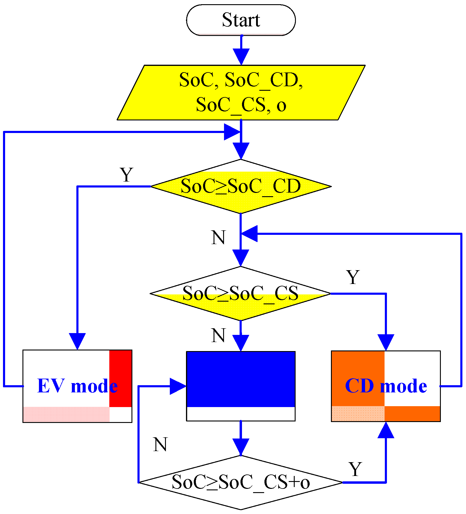
There are three kinds of energy consumption modes for PHSB, which are electric vehicle mode (EV), CD mode and CS mode. In this paper, the drive motor alone drives the vehicle during the EV mode, and all of the required energy for PHSB driving comes from the power battery packs. In the CD mode, both of the drive motor and the engine drive the PHSB, and the SoC of the power battery packs would be decreased gradually. In the CS mode, the engine provides most of the energy to drive the PHSB, and the SoC of power battery packs was maintained within an appropriate range until the PHSB stops. The energy consumption modes switching control strategy is shown in
Figure 6, where SoC_CD is the switch threshold between the EV mode and the CD mode, and SoC_CS is the switch threshold between the CD mode and the CS mode, o is the margin of switching back to CD mode from CS mode. In one PHSB trip, the mode switches constantly with the change of SoC, and EV mode switches to CD mode can’t be reversed unless the parking charge happens, but mode switch between CD mode and CS mode can be reversed when the SoC increases to a certain level.
Figure 6.
Mode switching control strategy.
Figure 6.
Mode switching control strategy.
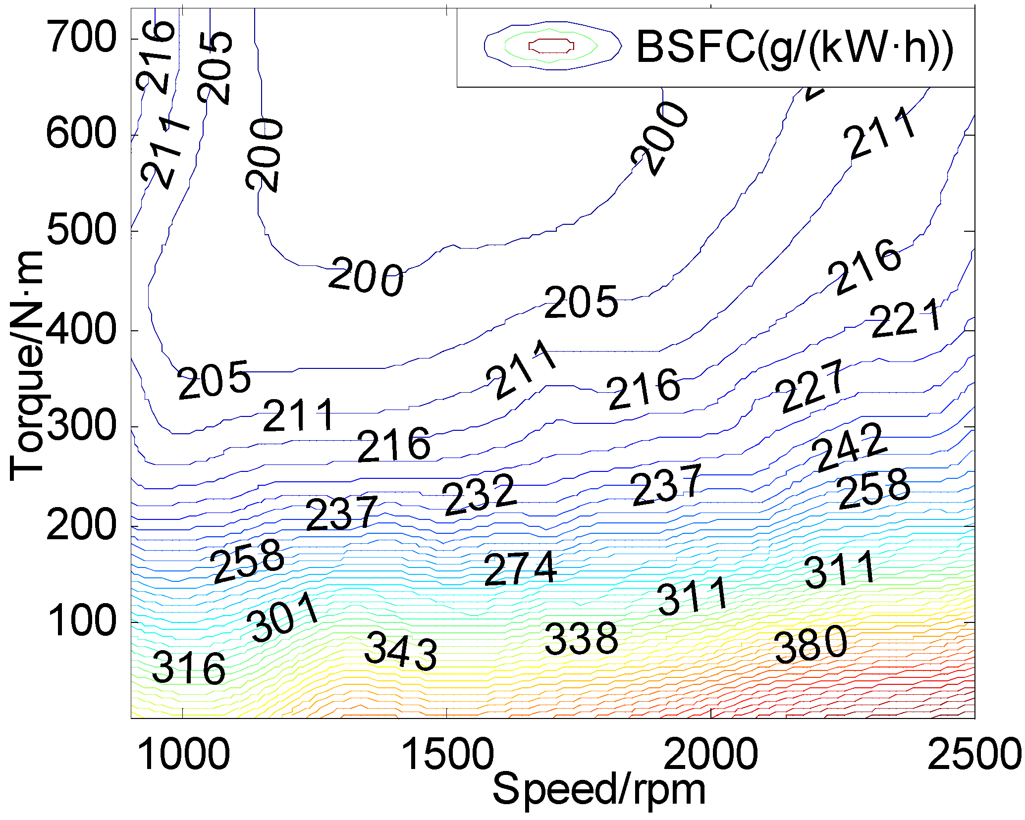
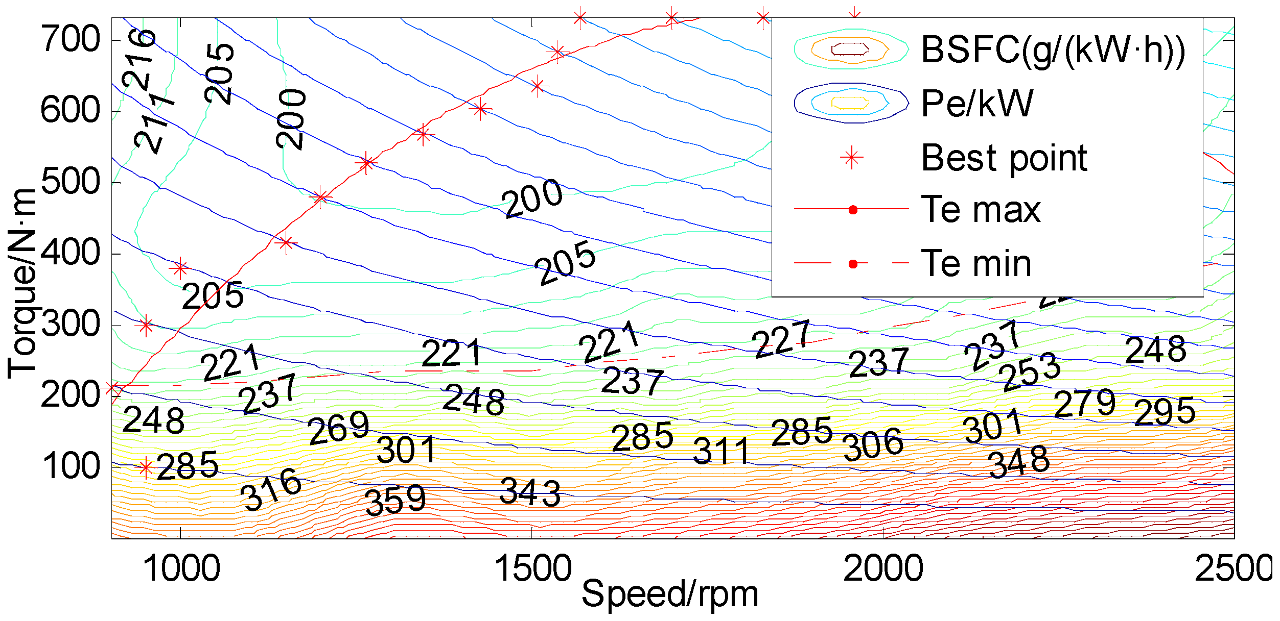
The selection of the engine optimal work area is mainly based on the engine optimal work curve. As shown in
Figure 7, the engine optimal work curve is fitted by the engine optimal work points, which correspond to the minimum fuel consumption and best fuel economy of the engine In this paper, Te_max(n) is the upper boundary of the engine optimal work area, which is the engine optimal work curve, and Te_min(n) is the lower boundary of the engine optimal work area, which is the 230 gp·kW·h fuel consumption contour. Therefore, the engine fuel consumption rate can be controlled below 230 gp·kW·h.
Figure 7.
Engine optimal work curve.
Figure 7.
Engine optimal work curve.
4.1. EV Mode
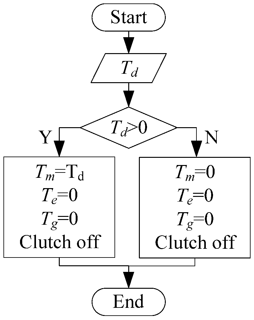
When SoC > 65%, the vehicle is in the EV (equivalent to a pure electric vehicle) mode. As shown in the
Figure 8, the energy is provided by the power battery packs at this time, and the driving demand is satisfied by the drive motor. In this mode, because of the higher SoC and the lower charge efficiency, regenerative braking is not performed to reduce the charge times and extend the power battery life.
Figure 8.
Energy management control strategy in EV mode.
Figure 8.
Energy management control strategy in EV mode.
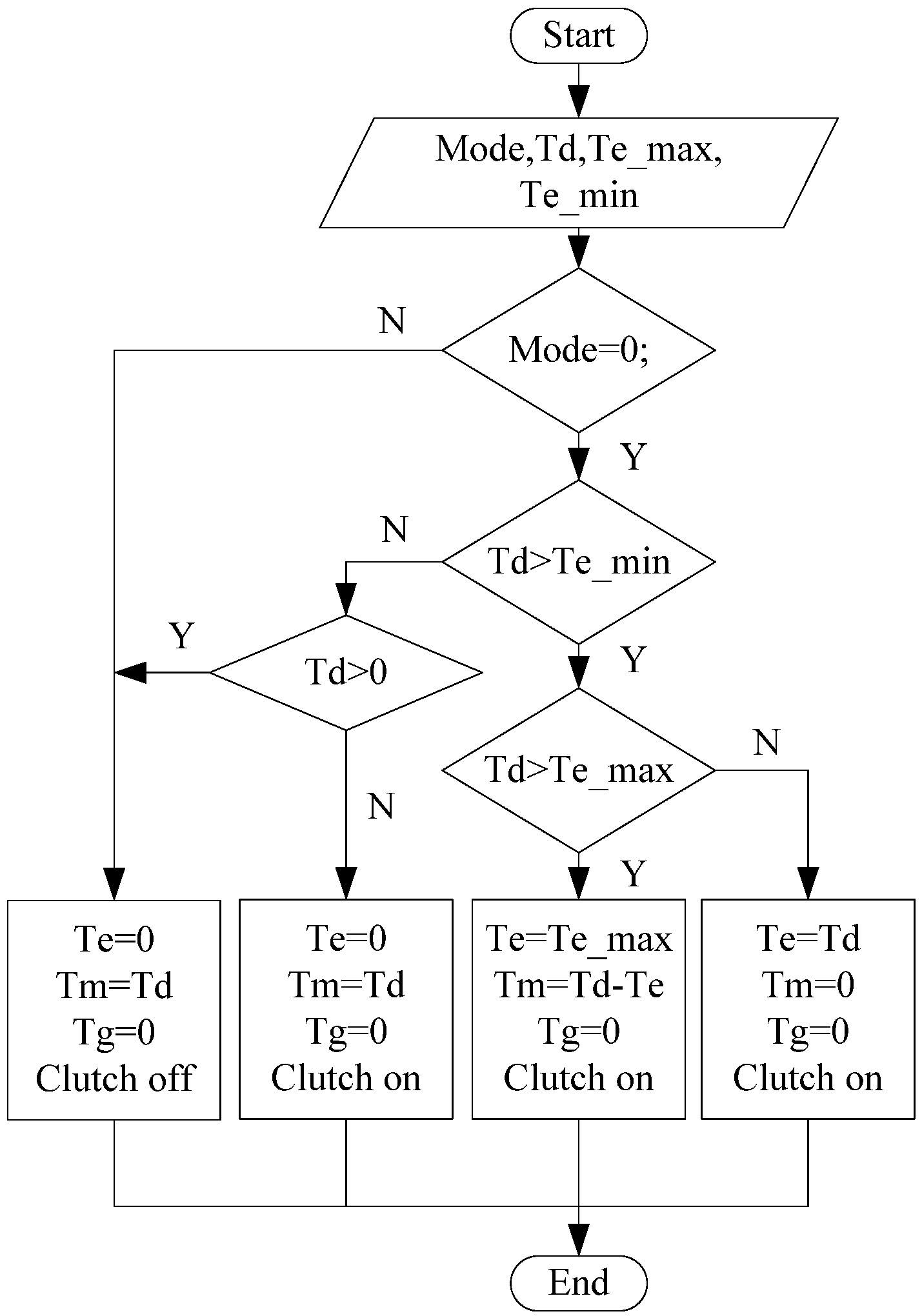
4.2. CD Mode
When 30% < SoC < 65%, it’s the CD mode and the corresponding control strategy flow is shown in
Figure 9. The PHSB is only driven by the drive motor when PHSB drives at a low speed. When the PHSB drives at a high speed, if the drive demand torque is less than the lower limit of the engine optimal work area, the engine shuts down, and the torque is provided by the drive motor; if the drive demand torque is in the engine optimal work area, the engine direct drive mode is adopted; if the drive demand torque is greater than the upper limit of the engine optimal work area, the engine and the main drive motor work jointly to meet driving demand. Regenerative braking can be employed to recover braking energy in CD mode.
Figure 9.
Energy management control strategy in CD mode.
Figure 9.
Energy management control strategy in CD mode.
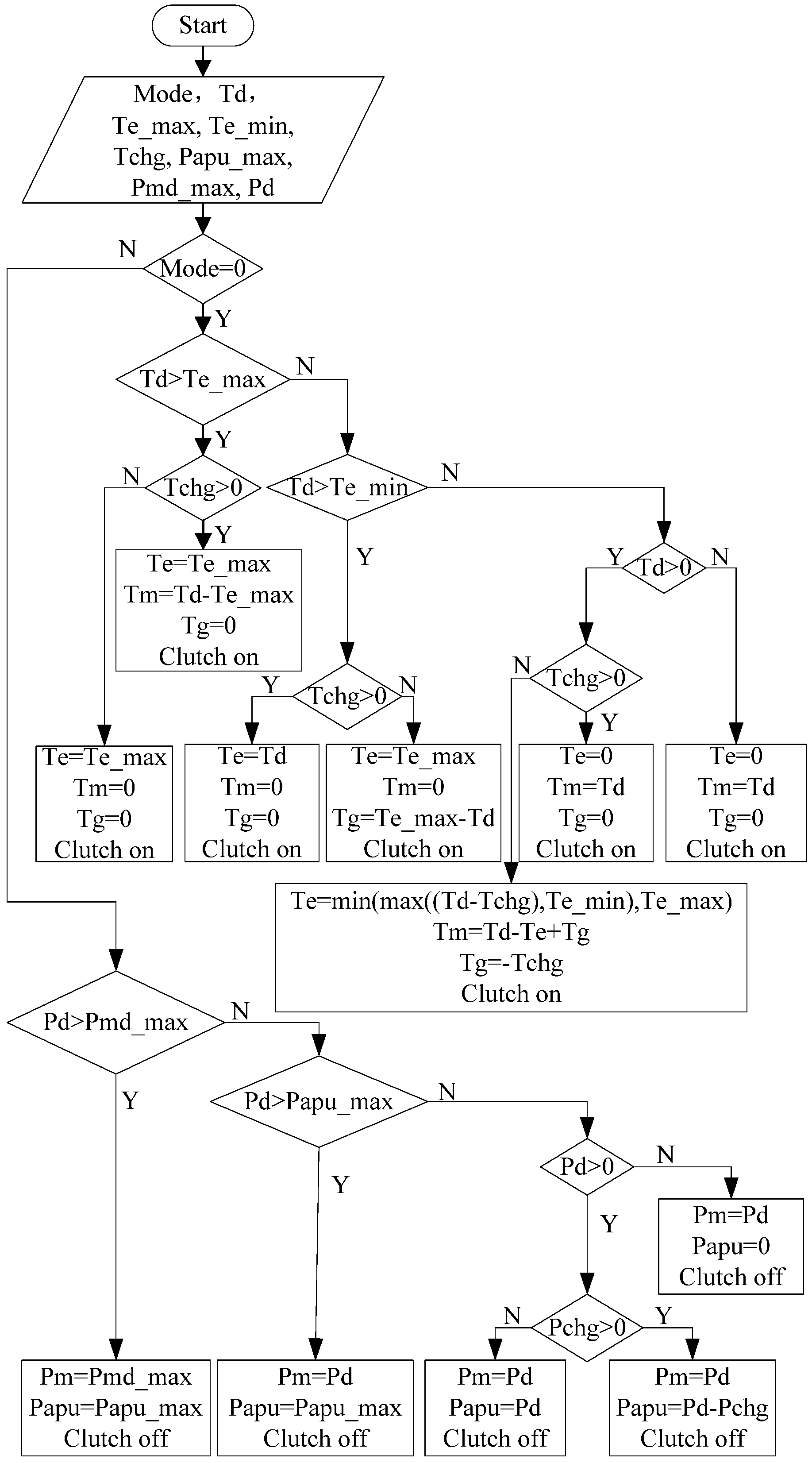
4.3. CS Mode
The control strategy follow of CS mode is shown in
Figure 10 as follows: when SoC < 35%, it is the CS mode. At this time, the control strategy needs to ensure the SoC is stabilized near 30%. The series hybrid mode is adopted when the PHSB drives at a low speed, and the demand power is satisfied by the drive motor.
Figure 10.
Energy management control strategy in CS mode.
Figure 10.
Energy management control strategy in CS mode.
If the power demand is greater than the APU maximum power, the APU works at the maximum power point; if the power demand is less than the APU maximum power but more than the lower limit of the APU and 30% < SoC < 31%, to minimize energy circulation, the APU output power is equal to the demand power; if the demand power is less than the APU maximum power but more than the lower limit of the APU and 29% < SoC < 30%, due to the power battery packs power shortage at this time, APU outputs the maximum power, meanwhile providing power to the drive motor and charging the power battery packs; if the demand power is less than the lower limit of the APU, APU works at the lower limit of the APU, it provides power to the drive motor and powers the battery packs at the same time, although it has energy circulation, it can be ensured that the engine works in optimal the work area, so the fuel consumption can be further reduced. This mode also allows regenerative braking to recover energy.
The series-parallel hybrid mode is adopted when PHSB drives at a high speed. When 30% < SoC < 31%, if the drive demand torque is less than the lower limit of the engine optimal work area, the demand torque is only provided by the drive motor, and the engine shuts down; if the drive demand torque is in the engine optimal work area, the engine direct drive mode is adopted; if the drive demand torque is greater than the upper limit of the engine optimal work area, the engine and the main drive motor work together to meet the running demand. Regenerative braking can be employed to recover energy in this mode.
When 29% <SoC < 30%, it needs to charge the power battery packs. If the drive demand torque is less than the lower limit of the engine optimal work area, the engine works in the engine optimal work area to drive the PHSB directly and start the ISG motor to charge the power battery packs; if the demand torque is in the engine optimal work area, the engine works at the upper limit of the engine optimal work area or the sum of the charge demand torque and demand torque, using the engine to drive directly and start the ISG motor to charge power battery packs; if the drive demand torque is greater than the upper limit of the engine optimal work area, the engine works atthe upper limit of the engine optimal work area to drive the bus, and the drive motor does not participate in the drive process. It also allows regenerative braking to recover energy in this mode.
5. Co-Simulation Experiments
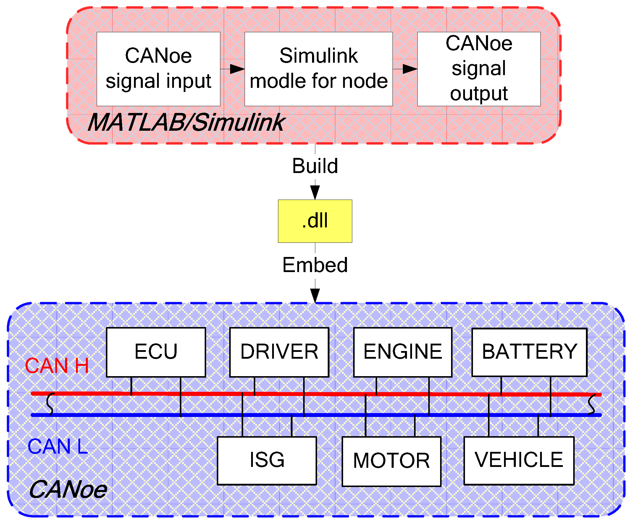
CANoe is a CAN bus simulation and test software that by using the CANdb++ database can simulate the communication protocol of the CAN bus. Although the control algorithm design and the control of CAN communication for each node can be realized in CANoe by using CAPL language, it seems jumbled and complicated for complex control algorithm and CAN communication.
MATLAB/Simulink is easy to use for developing complex control algorithms, but it lacks the capability of modeling and simulating a CAN bus. Therefore, the open interfaces of CANoe for Simulink are used to combine these two softwares for co-simulation, and the effect of the specified control strategy in CAN environments can be observed. The co-simulation detailed principle and bus topology structure are shown in
Figure 11.
Figure 11.
The co-simulation schematic of plug-in school bus.
Figure 11.
The co-simulation schematic of plug-in school bus.
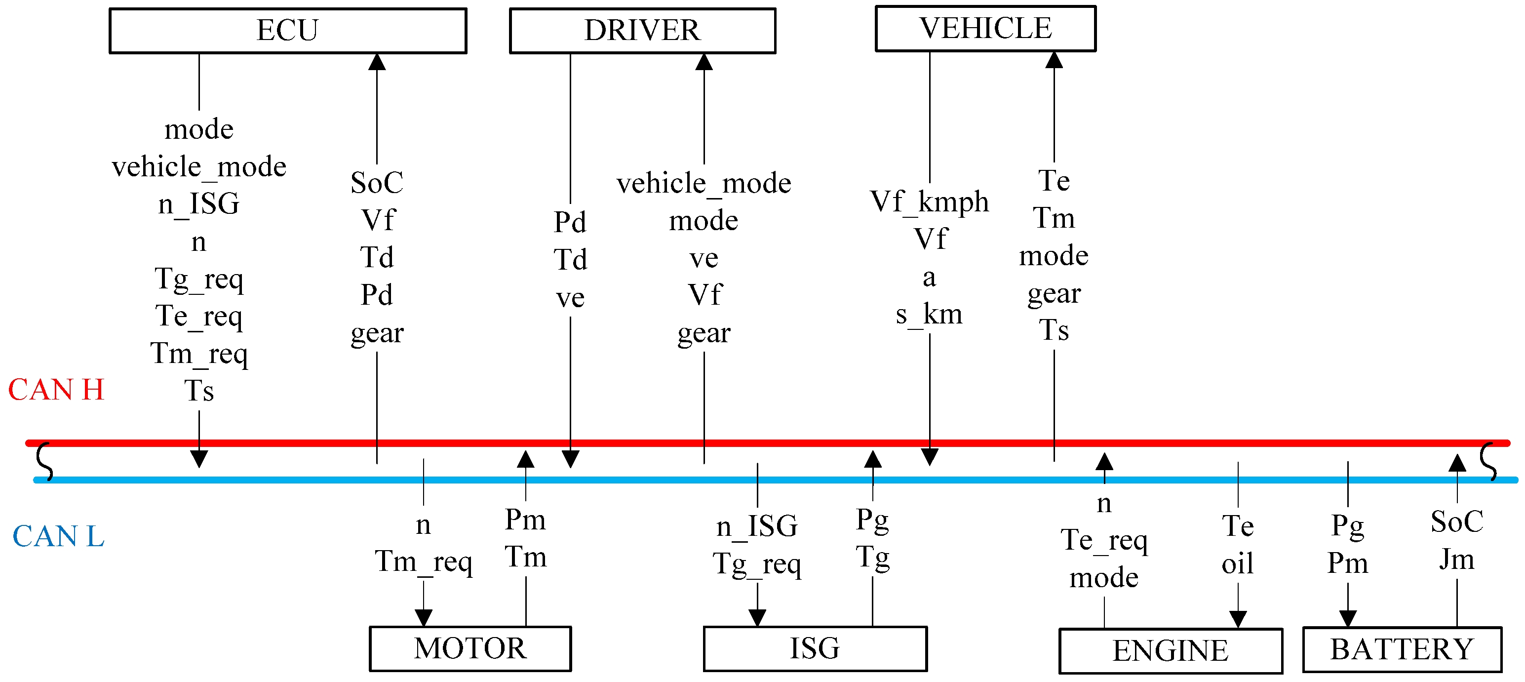
The co-simulation is carried out by using CANoe/Simulink, through the introduction of a simulated CAN bus connection to each sub-controller and vehicle model in the CANoe environment, the CAN bus load, signal delay and other characteristic parameters for the developed control strategy can be tested. The specific development procedures are as follows:
Firstly, the CANdb++ database was built, then the control strategy model was made a node, and all other power components models serve as individual nodes. The signals which are needed to transfer through the CAN bus associated with the sending and receiving messages of each node, and the completed setup database file was imported into a CANoe development panel. The signals of each node are as shown in
Figure 12.
Figure 12.
Nodes send and receive signals schematic diagram.
Figure 12.
Nodes send and receive signals schematic diagram.
Then, the input and output interfaces of models in Simulink of each control node were replaced with the corresponding Simulink/CANoe module interfaces, thus the signal association were completed. The models were converted into the .dll format control code through fast code generation technology, then the .dll file is embedded into the corresponding nodes of the CANoe development panel.
Finally, we verify whether the control strategy can send and receive signals according to the actual requirements by simulating the CAN bus environment, and observe the communication evaluation indexed like CAN bus load and so on, so as to complete the test and evaluation of the PHSB energy management strategy in the simulated CAN bus environment.
6. Simulation Results and Analysis
To verify the effectiveness and reasonability of the energy management strategy, several simulation experiments were carried out with the CANoe software. As shown in
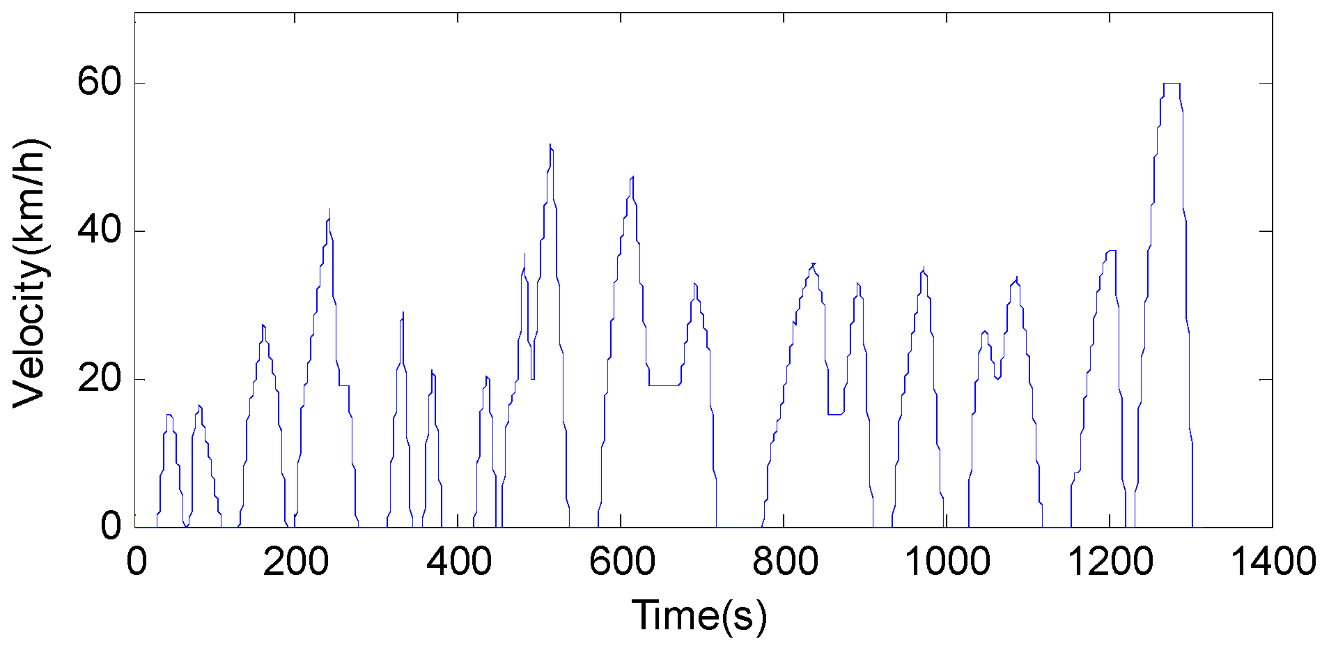
Figure 13, the Chinese typical city driving cycle is selected as the target velocity of the driver model.
Figure 13.
Chinese typical city driving cycle.
Figure 13.
Chinese typical city driving cycle.
In order to make the control strategy have a better display effect in this paper, three Chinese typical city driving cycles were run, however, wecan’t fully verify the mode switching of the control strategy by running only three Chinese typical city driving cycles, therefore, to reflect the three mode switches in the whole simulation process, the initial value of power battery packs SoC is set as 85%, the total capacity is reduced to 10 Ah, and the CAN bus baud rate is set as 500 kbs.
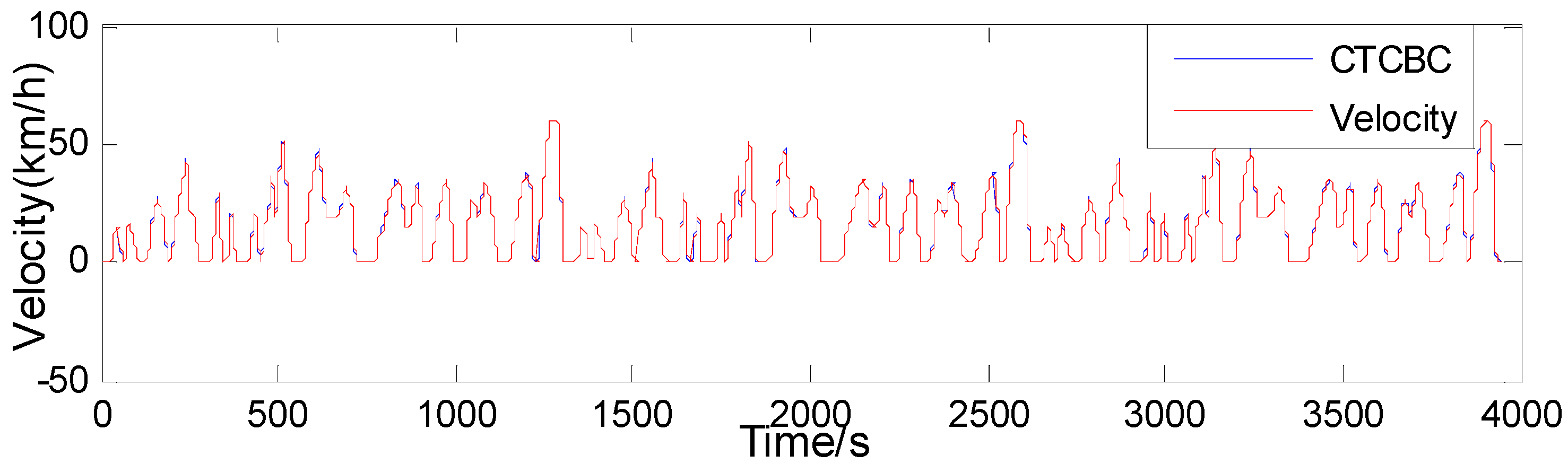
The effect of velocity following is shown in
Figure 14. The actual velocity can follow the velocity of the driving cycle well, and the requirements of the vehicle dynamic performance can be met, which indicates that the vehicle control strategy is reasonable and effective.
Figure 14.
The velocity following curve.
Figure 14.
The velocity following curve.
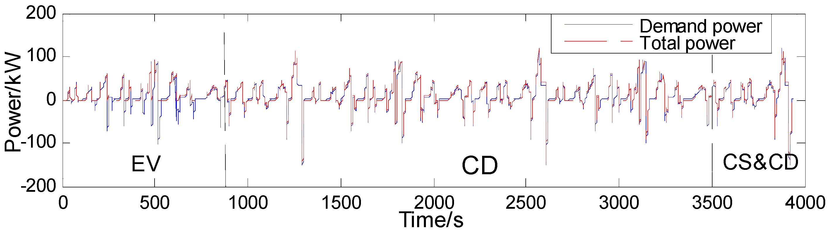
Figure 15 shows the power following between the total output power and the demand power. The results indicates that negative demand power does not coincide with the total output power before 870 s. The reason for this phenomenon is that the SoC is high in EV mode, and the designed control strategy does not allow charging and regenerative braking, so only the drive power can achieve a good follow effect. After 870 s, the work mode was changed into the CD and CS modes gradually, then the control strategy allows ISG motor generation and brake energy recovery, so that the total output power can better follow the power demand.
Figure 15.
The power following curve.
Figure 15.
The power following curve.
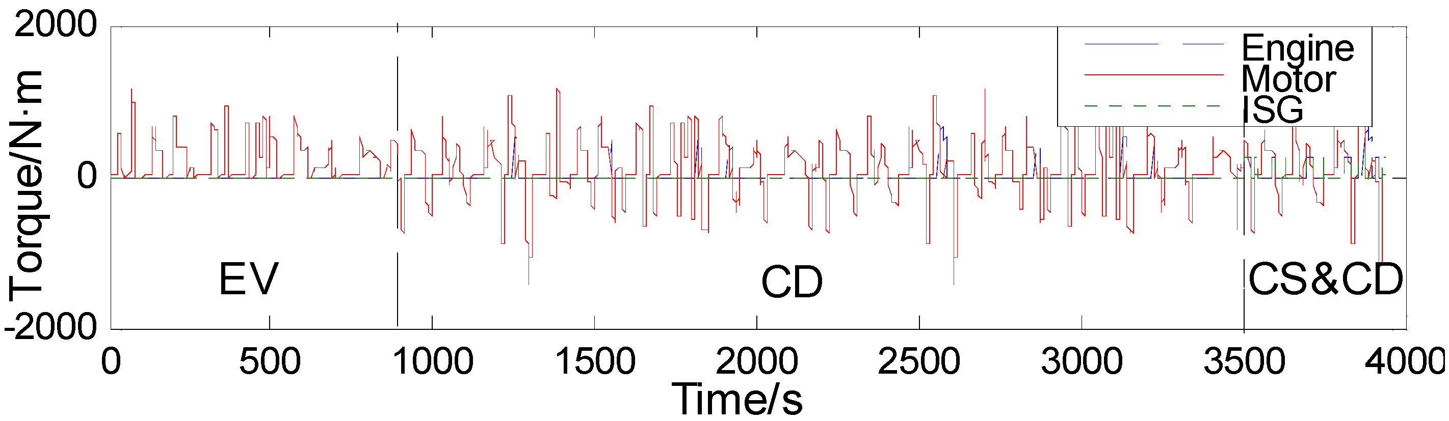
The work torque of power components is shown in
Figure 16. The engine does not work in EV mode, so the engine output torque is always 0; the ISG motor only works in CS mode, thus its torque is always 0 in the EV and CD modes; meanwhile in CS mode, the engine work range is larger than that in CD mode, due to the fact the engine not only provides the drive power in most stages, but also provides the generated power to the APU according to the control strategy in the CS stage, therefore, the engine output torque is greater than that in CD mode.
Figure 16.
Power components torque contrast.
Figure 16.
Power components torque contrast.
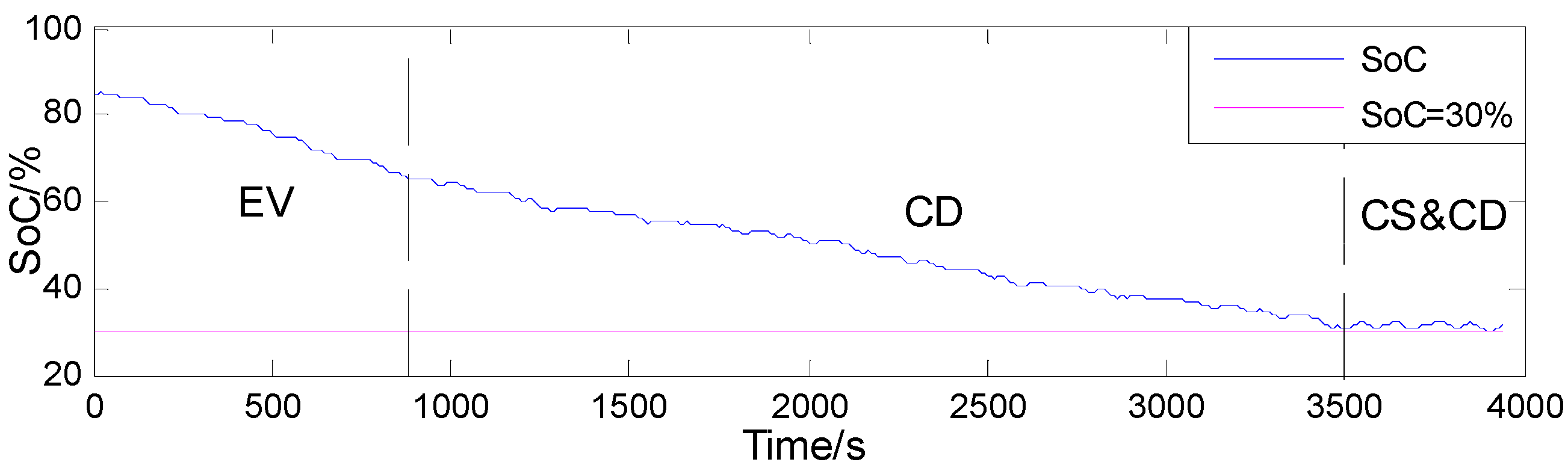
Figure 17 indicates that when the SoC is between 65% and 85%, the bus works in EV mode, without driving charging and regenerative braking, so the SoC doesn’t grow; the bus works in CD mode when the SoC is less than 65%, since this mode allows regenerative braking, the phenomenon that the SoC is increasing appears; when the SoC is less than 30%, the bus works in CS mode, SoC fluctuates between 29% and 31%, because the SoC change leads to the CD and CS mode switching, and finally makes the SoC fluctuate around 30%. It can be seen by the declining SoC slope, due to the fact the vehicle drive energy is not only from battery power, that the slope declines of SoC in CD and CS mode are slower than that in EV mode.
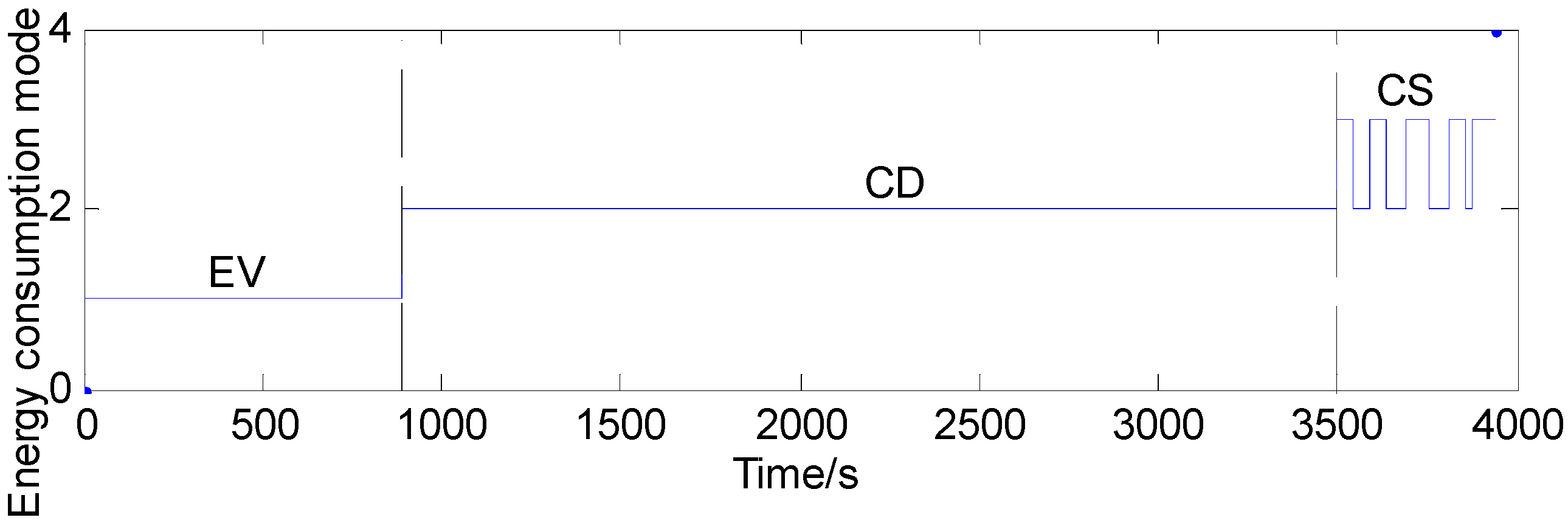
The energy consumption mode switch process of the control strategy is as shown in
Figure 18, and modes 1, 2, 3 represent EV, CS and CD modes, respectively. Combined with
Figure 17, it can be seen that, in accordance with the SoC change, switches between CD and EV mode can’t be reversed, but the switch between CD and CS mode is reversible. This results indicates that the designed control strategy can achieve CS and CD mode switching effectively during the subsequent PHSB travel, namely extending the use time of the CD mode, which is consistent with the control of objectives global optimization, and this is helpful for enhancing the fuel saving potential of the rule-based energy management control strategy.
Figure 17.
SoC change curve.
Figure 17.
SoC change curve.
Figure 18.
Energy consumption modes switch.
Figure 18.
Energy consumption modes switch.
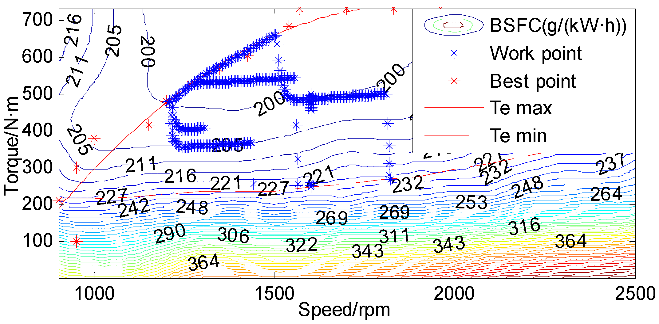
Figure 19 indicates that the engine work points (blue *) are always in the engine optimal work area, proving that the designed control strategy can obtain good fuel economy performance.
Figure 19.
Engine work points.
Figure 19.
Engine work points.
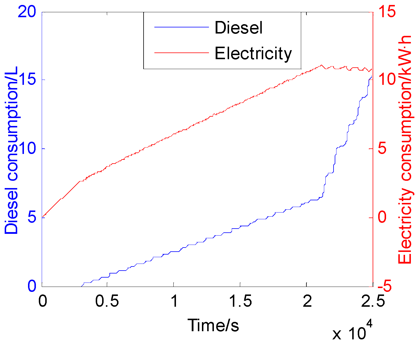
The battery capacity is restored to 72 Ah, and the SoC initial value is set as 75%, 19 Chinese typical city driving cycles were ran, and the resulting diesel consumption and electricity consumption are shown in
Figure 20, where the diesel consumption and electricity consumption are 15.3 L and 10.7 kW·h, which are equivalent to an energy consumption per 100 km of 13.7 L diesel consumption and 10.5 kW·h electricity consumption.
It can be seen from the above simulation results that the designed control strategy is reasonable and effective, the demand of PHSB dynamic performance can be guaranteed, meanwhile, the fuel consumption and power consumption reflect that the control strategy has good economic performance. If considering that the bus is running from the power battery fully charged state, due to the extended work hours of EV mode, the fuel saving effect will be more obvious.
Figure 20.
Diesel and electricity consumption.
Figure 20.
Diesel and electricity consumption.
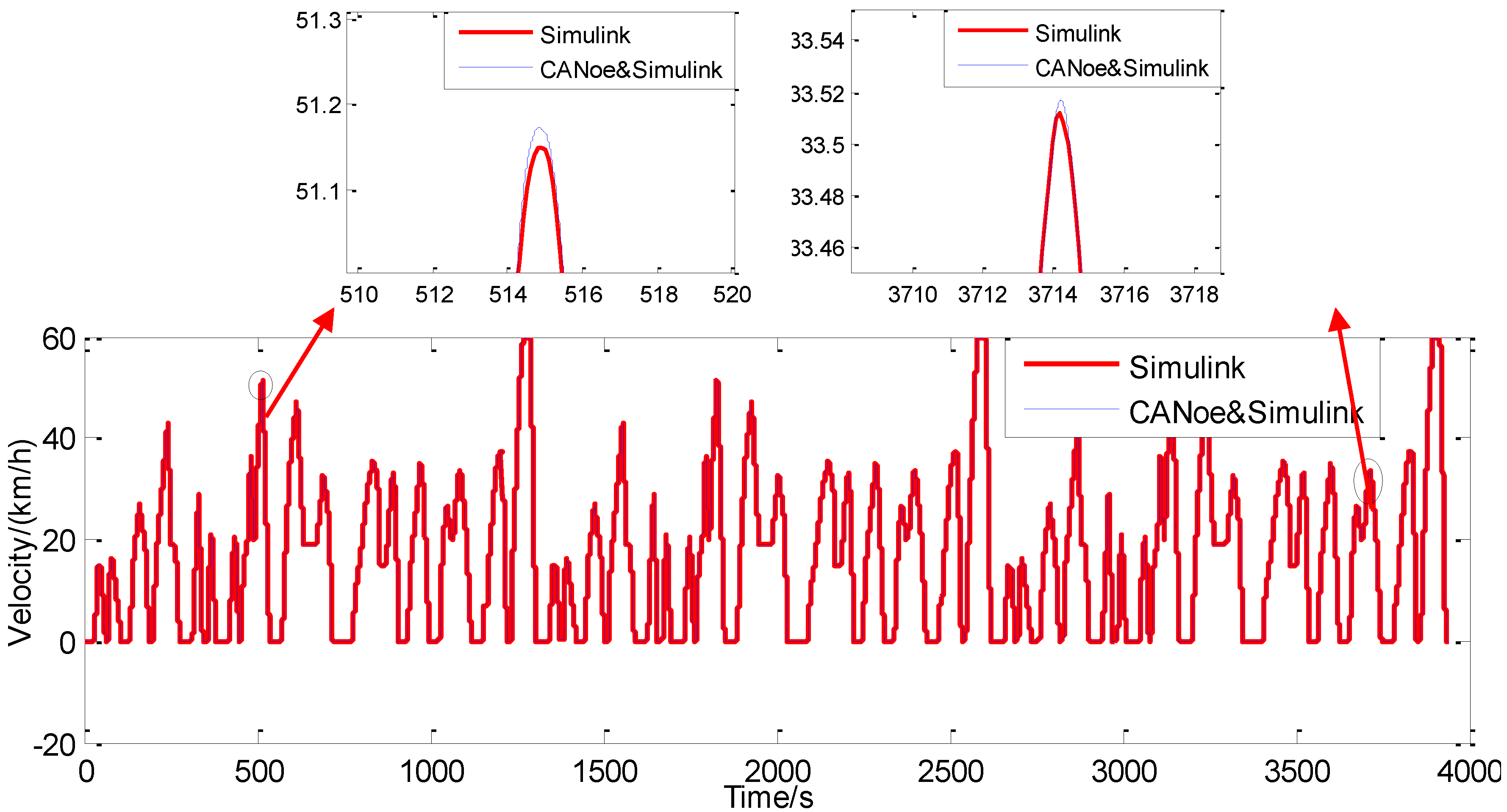
In order to detect the impact of the CAN bus performance indicators such as the load factor and signal delay on the control effect, a comparative velocity simulation was carried out with Simulink and CANoe. The comparison results are as shown in
Figure 21, where it can be seen that the two curves are basically the same.
Figure 21.
Velocity comparison from two kinds of simulations.
Figure 21.
Velocity comparison from two kinds of simulations.
It can be found by amplifying the details that the errors of the two simulation results during the rapid changes of the driving cycle are larger than at other positions, namely around the corner of the velocity curve. The communications between the nodes in Simulink are idealized, thus it’s not necessary to consider the delay response problems of the control signals. While in the CANoe environment, which adds the CAN bus simulation model, signals are transmitted at a fixed period between nodes through messages, so it can reflect the signals transmission process more truly. The power and torque of power components always change sharply at the rapid changes of the driving cycle, and the hysteresis effect of the simulation bus will enlarge the differences between the CANoe and Simulink simulation results.
For the velocity simulation results of CANoe and Simulink, 4000 sampling times’ velocities were selected randomly, and the error and the correlation coefficient between the two sets of sampling data are compared. The specific relevant indicators are shown in
Table 3.
Table 3.
Sampling velocity comparison.
Table 3.
Sampling velocity comparison.
| Parameter | Value |
|---|
| Maximum error (m/s) | 0.1071 |
| Minimum error (m/s) | 0 |
| Error standard deviation (m/s) | 0.0316 |
| Correlation coefficient | 0.98 |
| Determination coefficient | 0.96 |
The correlation coefficient can be used to represent the level of direct linear relationship intensity between the two sets of sample data, and the determination coefficient is the square of the correlation coefficient, which determines the close level of the comparative sample data, the correlation coefficient expression is as follows:
where
X represents the samples of the CANoe simulation results,
Y represents the samples of the Simulink simulation results.
It can be seen from the
Table 3 that there is close correlation between the two simulation results, and the impact caused by CAN communication delay is small. The evaluation parameters of CAN bus communication effect in CANoe software are shown in
Figure 22, which indicates that the CAN bus load rate maximum is 27.31%, less than 30%, thus it won’t cause a bus jam, the message delay is reasonable, the minimum interval for sending is 0 ms, 12 frames are sent each time, consistent with number of messages, the average transmission time is 2.710 s, and there are no error frames, no sending and receiving errors, so all the CAN communication properties meet the design requirements.
Figure 22.
The CAN communication evaluation parameters in CANoe.
Figure 22.
The CAN communication evaluation parameters in CANoe.
Note: n/a means the property parameter can’t be used in the corresponding analysis.
7. Conclusions
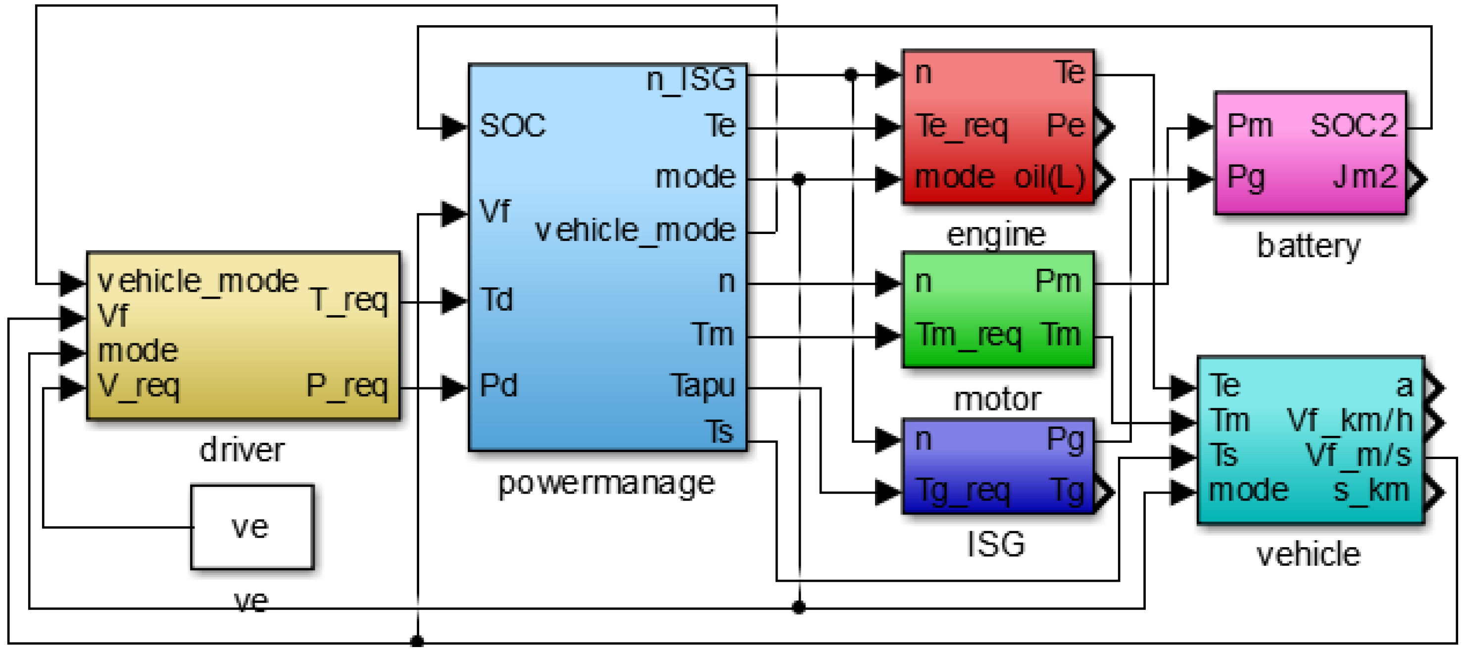
(1) In this paper, MATLAB/Simulink software is used to build a forward simulation model for a PHSB, and a rule-based energy management strategy is developed. In order to study the response of designed control strategy in the CAN bus environment, a simulation model of a singlet topology CAN bus is built with CANoe, and every model of the PHSB simulation model in the Simulink environment is separately imported to the corresponding node of the CAN bus simulation model through automatic code generation techniques.
(2) The Chinese typical city driving cycle is used as a target velocity, and several simulation experiments were carried out with CANoe. The simulation results show that the developed rule-based control strategy can follow well the target velocity and demand power, indicating that the developed control strategy can meet the requirements of PHSB dynamic performance. Meanwhile, it can realize CD mode and CS mode switching in the subsequent travel, and the SOC is stabilized around 30%. The energy consumption per 100 km is 13.7 L diesel and 10.5 kW·h electricity with an initial SoC of 75%, so the economy requirements of the PHSB can be guaranteed.
(3) The velocity comparison results between the Simulink/CANoe co-simulation and the Simulink individual simulation show that the correlation coefficient of the two sets of sampling velocities is 0.98, and the determination coefficient is 0.96, which indicates that the developed control strategy has a reasonable bus load and little delay effect. Co-simulation results shows that the bus communication is normal, there are no error frames, and each indicator of the bus communication is reasonable. The control strategy validation in the bus simulation environment shows that the developed control strategy has real-time and high reliability performance, so the study presented in this paper could lay the foundation for the hardware development of a vehicle controller.


