
Model-based Sensor Fault Diagnosis of a Lithium-ion Battery in Electric Vehicles

Collaborative Innovation Center of Electric Vehicles in Beijing, National Engineering Laboratory for Electric Vehicles, Beijing Institute of Technology, Beijing 100081, China
*
Author to whom correspondence should be addressed.
Energies 2015, 8(7), 6509-6527; https://doi.org/10.3390/en8076509
Submission received: 15 April 2015
/
Revised: 19 June 2015
/
Accepted: 19 June 2015
/
Published: 26 June 2015
(This article belongs to the Special Issue Advances in Plug-in Hybrid Vehicles and Hybrid Vehicles)
Abstract
:The battery critical functions such as State-of-Charge (SoC) and State-of-Health (SoH) estimations, over-current, and over-/under-voltage protections mainly depend on current and voltage sensor measurements. Therefore, it is imperative to develop a reliable sensor fault diagnosis scheme to guarantee the battery performance, safety and life. This paper presents a systematic model-based fault diagnosis scheme for a battery cell to detect current or voltage sensor faults. The battery model is developed based on the equivalent circuit technique. For the diagnostic scheme implementation, the extended Kalman filter (EKF) is used to estimate the terminal voltage of battery cell, and the residual carrying fault information is then generated by comparing the measured and estimated voltage. Further, the residual is evaluated by a statistical inference method that determines the presence of a fault. To highlight the importance of battery sensor fault diagnosis, the effects of sensors faults on battery SoC estimation and possible influences are analyzed. Finally, the effectiveness of the proposed diagnostic scheme is experimentally validated, and the results show that the current or voltage sensor fault can be accurately detected.
1. Introduction
The energy crisis and environmental issues regarding peaking petroleum production and greenhouse gas emissions have promoted the development of various kinds of electric vehicles (EVs). Lithium-ion batteries are attracting more and more attention as the energy storage system in today’s EV market, due to their inherent benefits of high power and energy density, long lifespan and low maintenance cost [1]. These growing demands make the battery performance and life of critical importance. To guarantee the battery performance, reliability and life, a battery management system is required to perform the critical functions like State-of-Charge (SoC) and State-of-Health (SoH) estimations, and over-current, and under-/over-voltage protection [2,3,4]. These critical functions rely deeply on embedded current and voltage sensor measurements. The sensors in the battery system may present different kinds of failures because of manufacturing defects, extended exposure to high temperature, and external shock or vibrations [5]. If the current or voltage sensor is faulty, the battery SoC and SoH estimations may be affected. An inaccurately estimated SoC acting in a role similar to that of a fuel meter for an internal combustion engine, may result in the battery suffering from over-charge or/and over-discharge [6]. This will accelerate the batter aging and decrease the battery life. Moreover, the current and voltage protection circuitries may be not working properly in the case of a faulty sensor. Therefore, it is imperative to develop a reliable and robust sensor fault diagnosis scheme for the lithium-ion battery that has been rarely addressed in the literature.
Data-driven and model-based fault diagnosis approaches are broadly applied in industrial applications [7]. The data-driven approach greatly depends on the analysis of extensive historical data to make a fault decision, but along with the major problems of time consumption, complexity of training, and computational cost [8]. However, model-based methods require an accurate mathematical model to capture the system process behaviors, and to help understand the underlying characteristics. With the benefits of low cost and high flexibility, model-based fault diagnosis has been extensively used to solve the challenge of accurate fault diagnosis in recent works. Observer-based fault diagnosis approaches further improve the robustness of model-based technique by avoiding the fault information loss due to the inaccurate initial value and unknown disturbance [9].
A bank of reduced order Luenberger observers (LOs) were applied to detect the variation of battery internal resistance in [10]. LO offers good performance under noise-free conditions, but in the presence of noise, it may face the challenge of achieving a satisfactory result. The nonlinear parity equation approach was used for a lithium-ion battery in a noise-free environment [11], but assuming the temperature data is always known. A multiple-model based fault diagnosis scheme was proposed for the lithium-ion battery to detect the over-charge and over-discharge with the use of a bank of extended Kalman filters (EKFs) in [12]. This method requires the identification of a healthy model, over-charge model and over-discharge model, and each model works in parallel with an EKF. The major problems of this approach may be attributed to the large computational demands of identifying each model and running a bank of EKFs. To the best of our knowledge, the topic of battery sensor fault diagnosis is still very rare.
In this paper, a systematic model-based fault diagnosis scheme is proposed for a lithium-ion battery cell to detect current or voltage sensor faults. This is just an example, and this methodology can be generally applied to any other faults of interest. For the diagnostic implementation, EKF is used to generate the residual carrying fault information. The use of EKF-based fault diagnosis shows good capabilities of noise robustness and guaranteeing accurate fault decisions [13,14,15,16,17]. It provides the benefits of detecting a fault at an early stage, decoupling the faults of interest from others, and minimizing the influences due to the model uncertainties and unknown disturbances. Besides, EKF can achieve a good diagnostic performance with the inherent benefits of being easily implementable and offering less computational complexity. Despite these potential benefits, EKF has not been used for the critical topic of battery sensor fault diagnosis. Further, the generated residual is evaluated by a statistical inference method that determines the presence of a fault. Moreover, to emphasize the importance of battery sensor fault diagnosis, the effects of sensors faults on SoC estimation are analyzed. Finally, the effectiveness of the proposed diagnostic scheme is experimentally validated under two different driving cycles, and the results show the current or voltage sensor fault could be accurately detected.
The rest of this paper is organized as follows: Section 2 describes the battery modeling, while Section 3 presents the model-based fault diagnosis scheme. Section 4 gives the battery experimental design and model identification results, and Section 5 analyzes the effects of sensors faults on battery SoC estimation. The diagnostic experimental evaluation and resulting conclusions are given in Section 6 and Section 7, respectively.
2. Battery Modeling
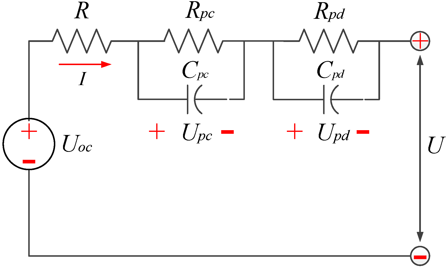
For modeling a lithium-ion battery, different kinds of techniques have been proposed in the literature like electrochemical, experimental, neutral networks, and equivalent circuit modeling [2]. In particular, the equivalent circuit models (ECMs) are the most commonly used approaches for control-oriented applications due to their good representation of cell dynamics and less computational demands. A comprehensive study of different order ECMs was presented, showing that higher order models have a better representation of the electrochemical phenomenon but at the expense of a higher computational demand [18]. To balance the model accuracy and computational demands, the second order ECM is used in this work. The model, as shown in Figure 1, is composed of an open circuit voltage (OCV) Uoc, an ohmic resistance R, and two parallel RC networks (Rpc-Cpc, and Rpd-Cpd). The Rpc-Cpc network represents the interfacial impedance of the cell, while the Rpd-Cpd network depicts the local properties of the electrode. The equivalent circuit parameters are dependent on the battery SoC, temperature and aging. In this study, the battery operation temperature is assumed to be constant and the battery aging is not considered. The model representations with the Kirchhoff’s voltage law are given by:
where I is the current that is positive at discharge and negative at charge; U is the cell terminal voltage; Upc is the voltage drop across the capacitor Cpc; and Upd is the voltage drop across the capacitor Cpd.
Figure 1.
Second order equivalent circuit model.

The battery OCV is usually a nonlinear function of SoC, and it can be expressed as:
The nonlinear relationship can be calibrated through experimental tests. The battery SoC is defined as the ratio of the remaining useful capacity to the total available capacity [2]. The SoC calculated by Coulomb counting can be expressed in the discrete form as:
where Cn is the battery nominal capacity in Ampere-hours; η is the coulomb efficiency assumed to be 1 at charging and 0.98 at discharging as the battery works in a limited current range; k is the time index; and Δt is the time interval.
Using the zero-order hold (ZOH) discretization method [19], the discrete time form of model dynamics are given by:
For a nonlinear time invariant system [20], the dynamics in discrete time are expressed as:
where wk and vk are an independent, zero mean, Gaussian process and measurement noise of covariance Qk and Vk, respectively; g(xk, uk) is the nonlinear system process function; and h(xk, uk) is the nonlinear measurement function.
The state variables for the battery cell are defined as xk = [Upc(k) Upd(k) SoC(k)]T, and the functions g(xk, uk) and h(xk, uk) can be expressed as:
3. Model-based Fault Diagnosis Scheme
Model-based fault diagnosis requires an accurate mathematical model to represent the system processes. This process model should show a good agreement with the system dynamics, and meanwhile it should be used to generate residual by comparing the model response and measured process output. Thus, there may be some errors in the residual because of inaccurate initial values, and unknown disturbances. To surmount this issue, the process model and subsequent residual generation process are replaced by the state observables, which is called observer-based fault diagnosis [7].
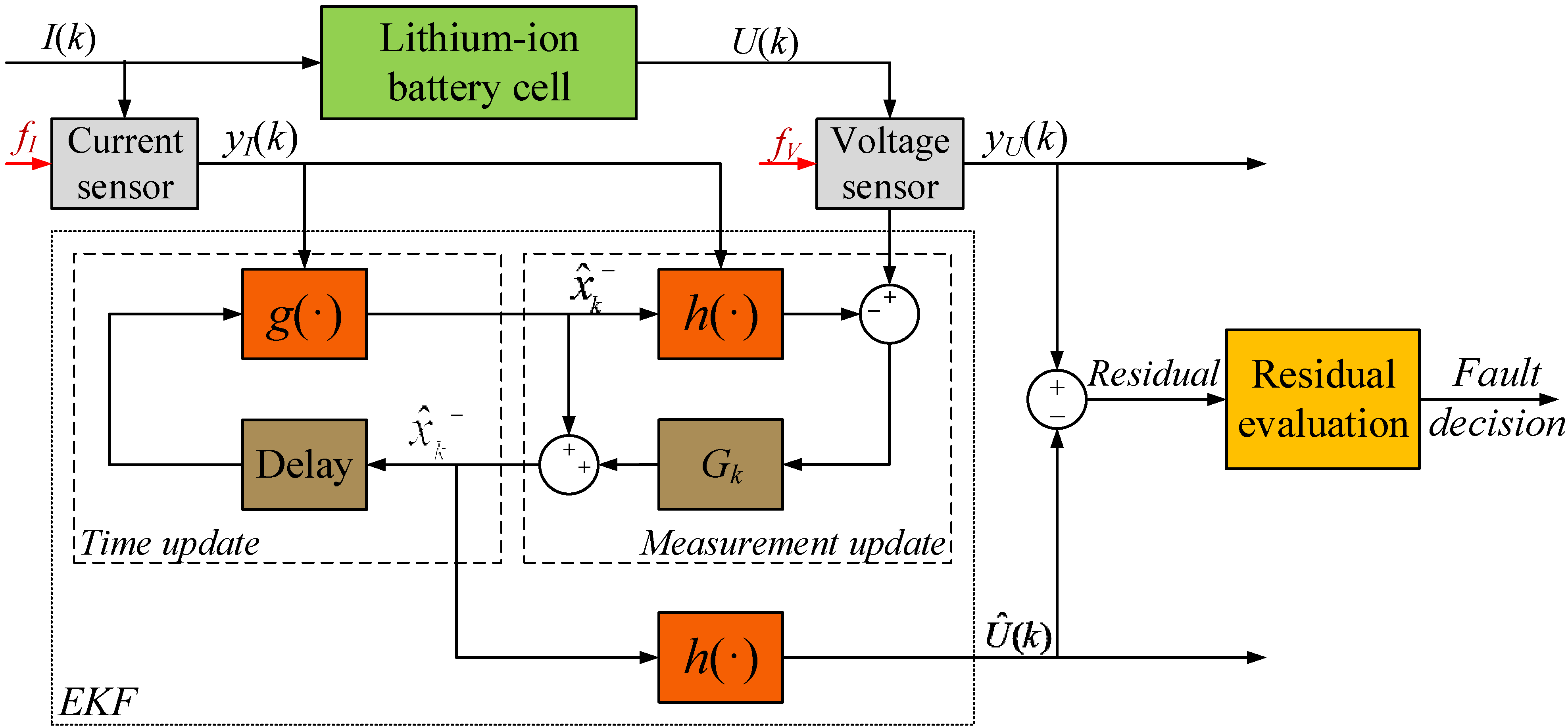
The general configuration of EKF-based fault diagnosis is shown in Figure 2. EKF works in parallel with the lithium-ion battery cell, and based on the measured input current and output voltage, the battery states are estimated. The estimated states are used to further predict the battery output voltage Û(k). The residual with the fault information is then generated by comparing the EKF-estimated and measured output voltage. To make a reliable fault decision, the generated residual will be evaluated by a statistical inference method. In this work, it is assumed that only one sensor fault is present at a time.
Figure 2.
Schematic of the proposed fault diagnosis.

3.1. Considered Sensor Fault
Most of the current and voltage sensors used in the battery systems of EVs are Hall effect sensors, which are subject to bias (offset) and gain fault (scaling) [3]:
Bias is a constant offset from the nominal statistics of the sensor signal. The current sensor is usually subject to bias faults, that may be caused by flaws in the sensor core such as degradation or breakage, and abrupt current changes [5].
Gain fault (scaling): magnitudes are scaled by a factor where the form of the waveform itself does not change. Gain faults are assumed to occur in the voltage sensor. This fault mode may present due to long exposures to high temperatures, and external shock or vibrations [5].
In industrial application, it has been demonstrated that the bias and gain faults could be considered additive faults that are commonly modelled as [5,14,16]:
where yx is the current or voltage sensor measurement; x is the battery input current I or terminal voltage U; and fx is the current fault or voltage fault value.
3.2. Extended Kalman Filter Design
For a nonlinear system, the basic idea of EKF for state estimation is to linearize the nonlinear dynamics around the current mean and covariance [20]. The time update equations to calculate the a priori estimations for the states and error covariance are given by:
while the measurement update equations to correct the a priori estimation for the state and error covariance to get an improved a posteriori estimation, are defined as:
where is the a priori state estimate at step k; is the a priori covariance estimate at step k; represents the updated a posteriori state estimate; is the updated a posteriori covariance estimate; and Gk is the Kalman gain. For the battery dynamics, the Jacobian matrix Ak and observation matrix Ck are given by:
The estimated output voltage is expressed as:
Then the residual carrying the fault/or fault-free information, can be generated by comparing the estimated and measured output voltage defined as:
where r is the generated residual; and yU(k) is the measured terminal voltage. Assuming there is no measurement noise and modelling error, the residual r would be zero in the sensor fault-free case; the residual r = 0 will be violated if a fault occurs.
3.3. Residual Evaluation
Due to the existing modelling error and measurement noise, the residual would be non-zero even under healthy sensor conditions, therefore, the conventional residual evaluation methods like constant thresholding would be not sufficient to evaluate the residual. To reduce the false alarms or missed detection instances, a statistical cumulative sum (CUSUM) test is applied [21]. The CUSUM test is to test two hypotheses H0 and H1 against each other to determine which of them describes the observed data, where H0 and H1 represent the no-fault and faulty case, respectively. The cumulative sum of the log-likelihood ratio of an observation z is defined as:
where z(i) is the Gaussian distributed observed signal, i.e., the residual r; s(·) is the log-likelihood ratio; S(k) is the cumulative sum of the log-likelihood ratio, and it will be increasing during the fault occurring. pH1 and pH0 are the probability density function in the faulty and fault-free case, respectively; H1~N(μ1, σ12) and H0~N(μ0, σ02).
If both the mean and variance of the residual change, the log-likelihood ratio s(z) is derived as:
The fault decision logic is defined as:
where J is the pre-defined threshold that is calibrated through experiments. For the fault flag, “1” means there is a fault, while “0” means there is no fault.
4. Experiment Design and Model Identification
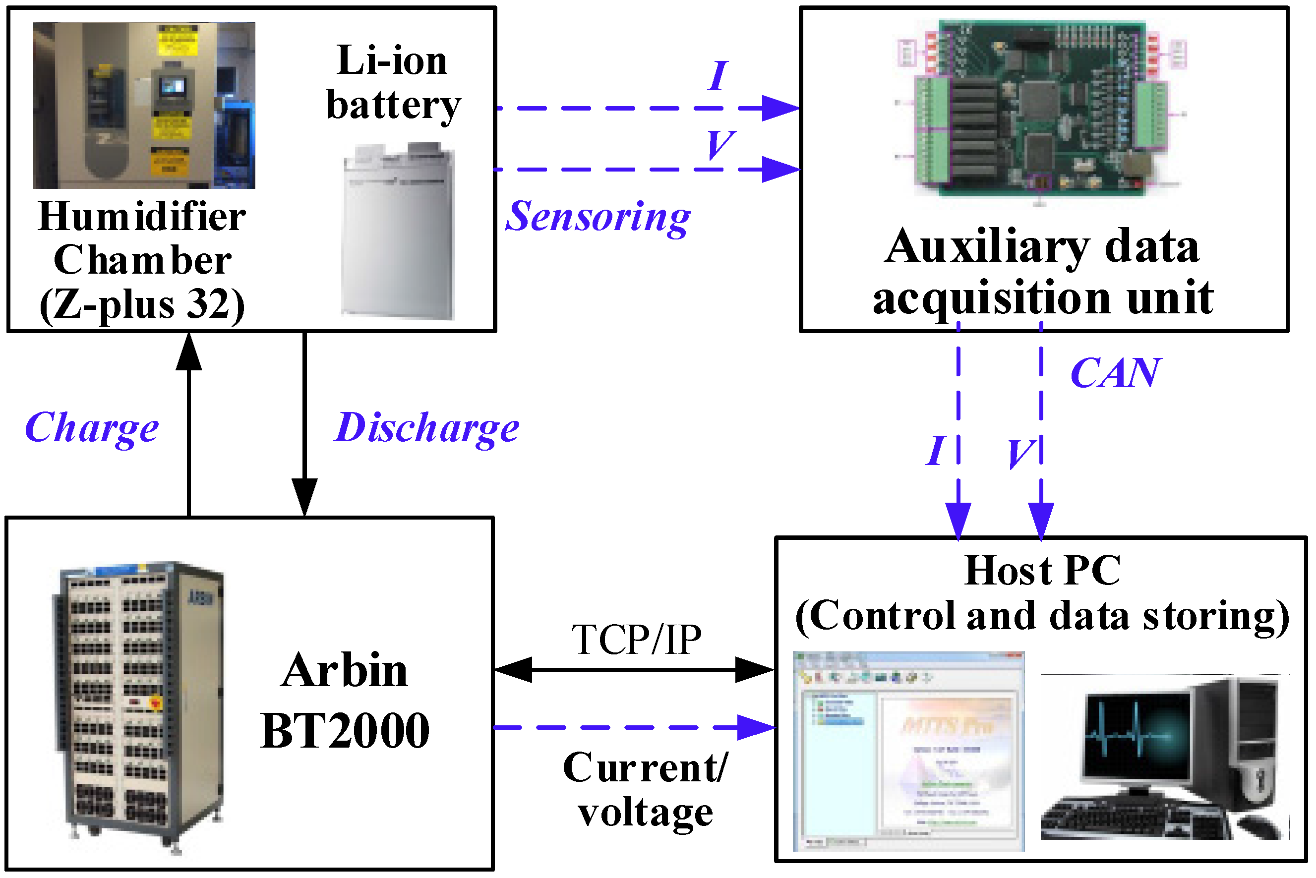
The aim of this section is to identify the battery model through experimental tests before implementing the diagnostic scheme. Experiments have been conducted on a manganese-based lithium-ion battery cell with the rated capacity of 32 Ah and nominal voltage of 4.2 V. The battery experimental setup, as shown in Figure 3, is composed of a battery test system (Arbin BT 2000), a humidifier chamber (CSZ’s Z-plus 32) to provide a controlled environment with temperature ranging from −55 °C to 85 °C, an auxiliary data acquisition unit to collect the measured signals, and a computer with Arbin’s MITS Pro software used for controlling the battery test system and storing the data. The BT 2000 is used to charge and discharge the battery according to the designed program with a maximum current of 300 A and maximum voltage of 60 V, and it can also record the current, voltage data, as well as Amp-hours (Ah) etc. The current and voltage data also can be collected by the auxiliary acquisition unit. The current and voltage data was recorded with a sample frequency of 10 Hz at the temperature 25 °C. The recorded current is taken as positive at discharge and negative at charge. To guarantee the initial SoC is always known, prior to each test, the battery was charged to 100%.
Figure 3.
Schematic of the battery test bench.

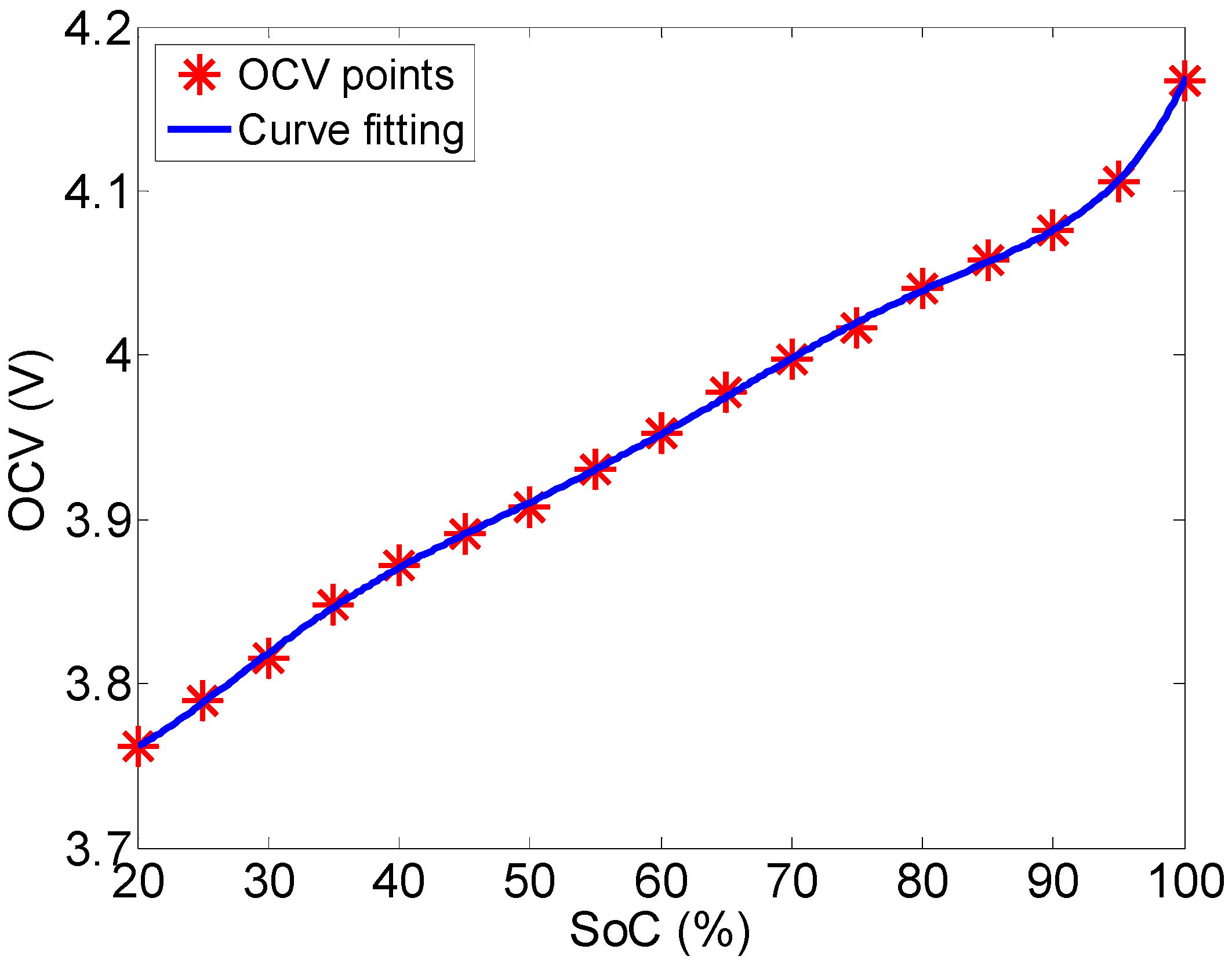
The tested available capacity is around 30.86 Ah. Through experimental tests, the recorded OCV data at each given SoC were obtained and plotted in Figure 4. The OCV-SoC relationship can be captured by a sixth order polynomial function given by:
where a1 = 36.43, a2 = −123, a3 = 165, a4 = −111.5, a5 = 39.48, a6 = −6.36, a7 = 4.12. The detailed processes of the capacity and OCV tests can be found in [22].
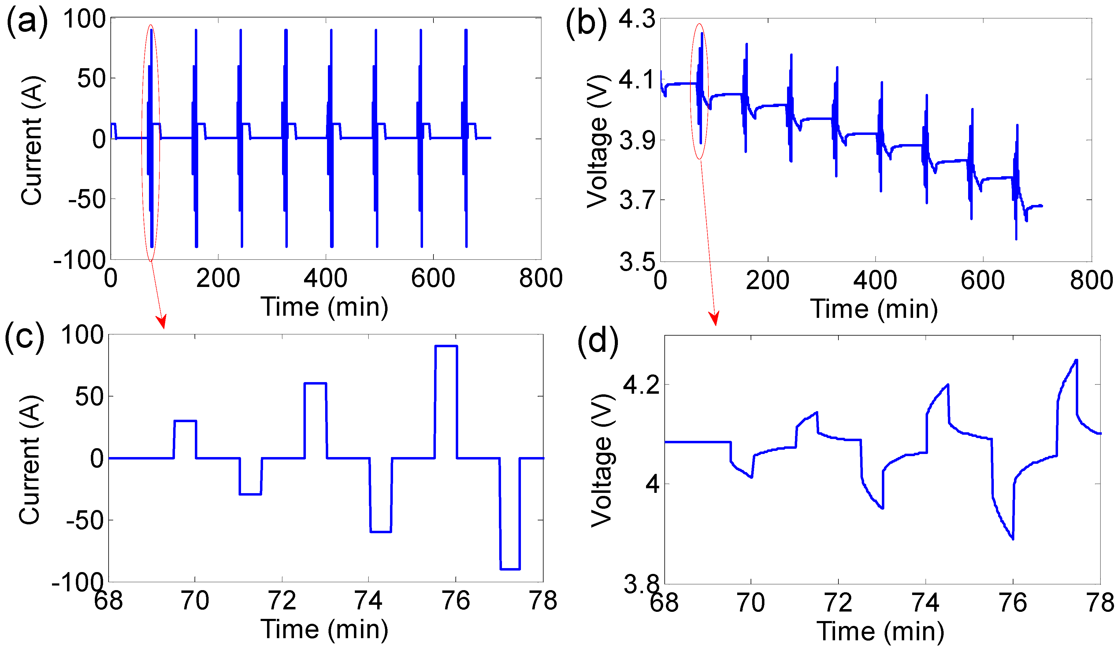
The hybrid pulse test was performed to identify the equivalent parameters R, Rpc, Cpc, Rpd and Cpd at each given SoC [22]. Figure 5a,b show the input current and corresponding voltage, while Figure 5c,d plot the amplified current pulses and voltages at 90% SoC. To identify these parameters, the recursive least squares with forgetting factor technique is used.
Figure 4.
Recorded OCV points and curve fitting results.

Figure 5.
Hybrid pulse test. (a) Current demand; (b) Corresponding voltage; (c) Current pulses at SoC 90%; (d) Voltage of current pulse at SoC 90%.
Figure 5.
Hybrid pulse test. (a) Current demand; (b) Corresponding voltage; (c) Current pulses at SoC 90%; (d) Voltage of current pulse at SoC 90%.

4.1. Equivalent Circuit Parameters Identification
Compared to the standard recursive least squares (RLS), the RLS with forgetting factor (RLSF) can give less weight to the older data and more weight to more recent data, which is appropriate for time-variant parameter identification [19]. The system to be identified can be expressed in the discrete time form as:
where y(k) is the observed battery voltage, θ is the parameter vector to be identified, and φ(k) is the regressor matrix with the observed current and voltage data.
Equations (6) and (7) can be represented as:
The voltage difference Ud = U-Uoc is considered as the OCV has been obtained. Then y(k) in Equation (26) would be Ud(k). Equations (8) and (27) through the z-transformation can be written as:
Through the inverse z-transformation, Equation (29) is rewritten as:
The parametric form for the battery model is given by:
The RLSF estimation equations can be illustrated as:
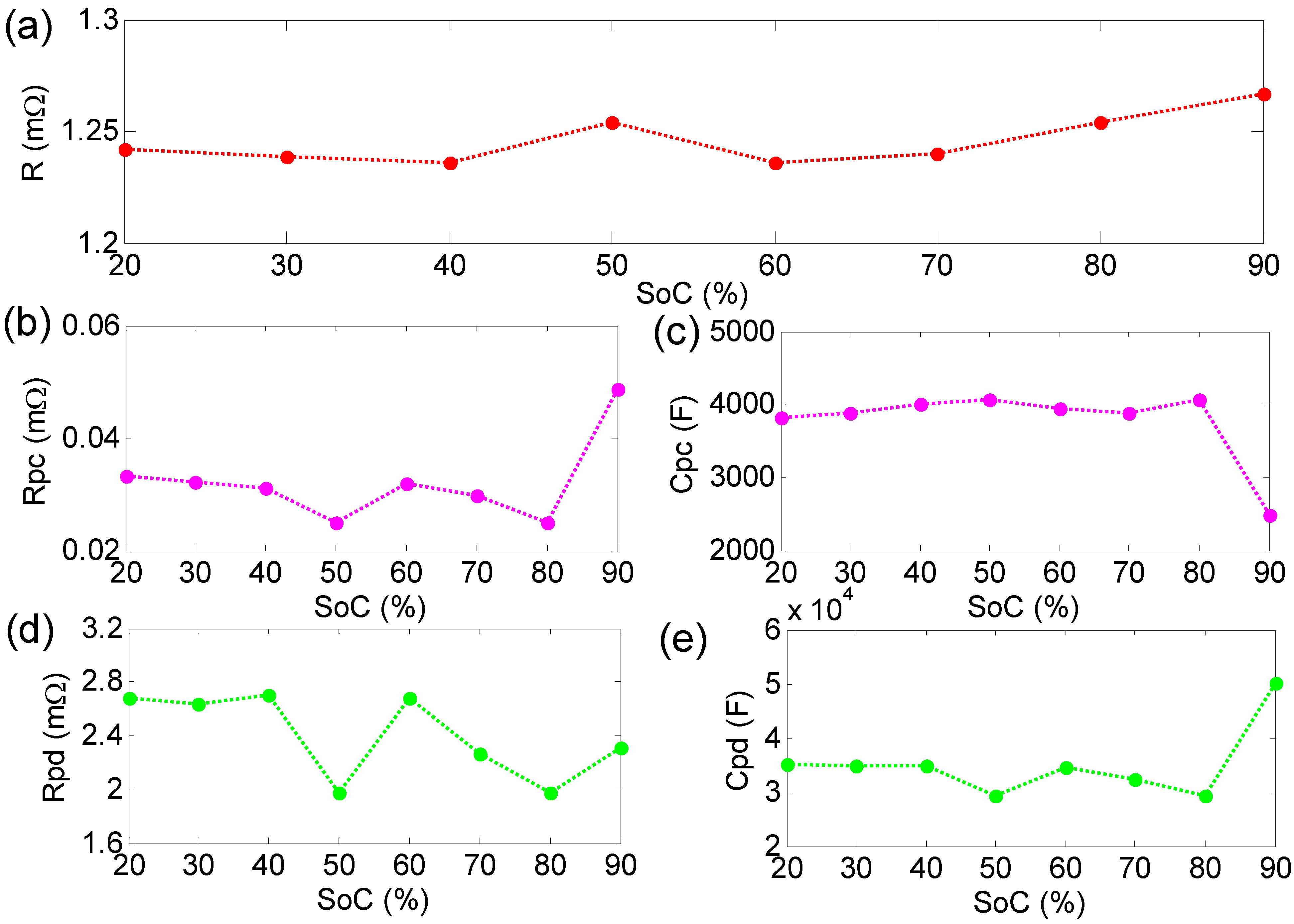
where Ud(k) is the observed voltage difference; P(k) is the covariance matrix; K(k) is the algorithm gain; and λ is the forgetting factor, 0< λ ≤ 1. The identified parameters at SoC from 20% to 90% are plotted in Figure 6.
Figure 6.
Parameters identification results. (a) Identified R; (b) Identified Rpc; (c) Identified Cpc; (d) Identified Rpd; (e) Identified Cpd.
Figure 6.
Parameters identification results. (a) Identified R; (b) Identified Rpc; (c) Identified Cpc; (d) Identified Rpd; (e) Identified Cpd.

4.2. Model Validation
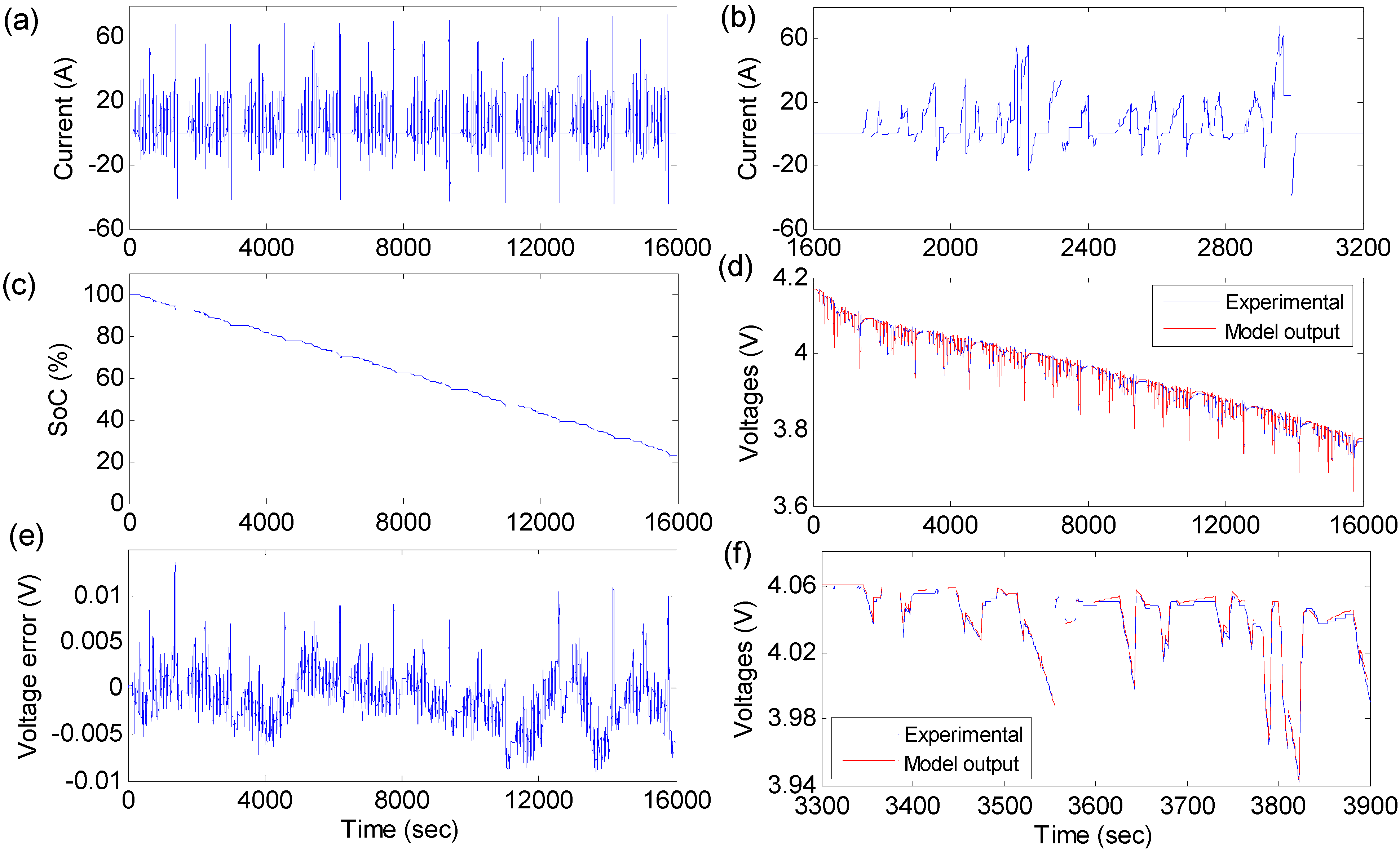
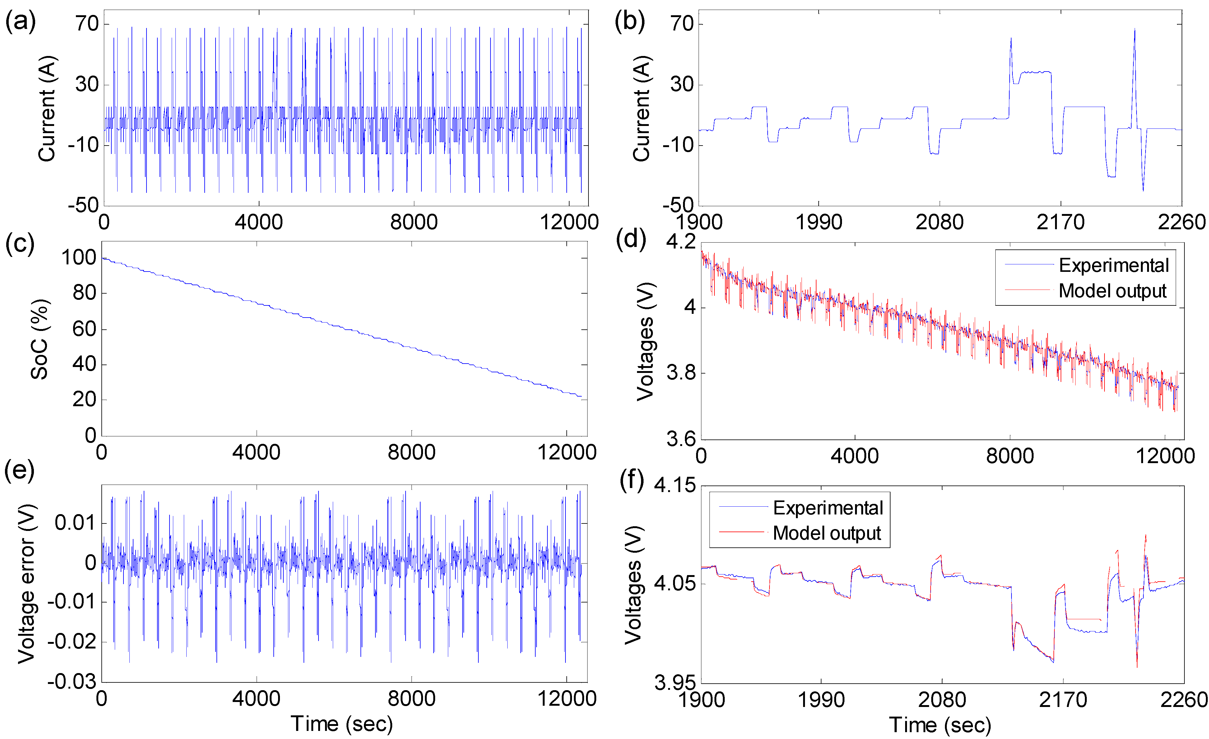
The scaled Urban Driving Cycle (UDC) and Dynamic Stress Test (DST) are used for the battery to simulate the actual driving cycles of EVs. These driving cycles were firstly performed to validate the model with the identified parameters. Figure 7 shows the model validation results under the ten UDC cycles, and the initial SoC is set to 1. Figure 7a–c plots the input current, amplified current of one driving cycle, and SoC trajectory, respectively. Figure 7d shows the comparison of experimental and model output voltage, while Figure 7e plots the voltage error. It can be found that the maximum error is around 0.012 V. Figure 7f plots the amplified portion of experimental and output voltages showing more details. The root mean square (RMS) value under ten UDC cycles is around 27 mV. Similar results under DST test are plotted in Figure 8. The maximum absolute error is around 0.025 V, while the RMS value is 20.6 mV. According to the results, it can be concluded that the model could accurately capture the cell dynamics, and it is suitable to be used for model-based fault diagnosis.
Figure 7.
Model validation under UDC test. (a) Input current profile; (b) Amplified current of one driving cycle; (c) SoC trajectory; (d) Comparison of experimental and model output voltages; (e) Voltage error; (f) Amplified experimental and model output voltage.
Figure 7.
Model validation under UDC test. (a) Input current profile; (b) Amplified current of one driving cycle; (c) SoC trajectory; (d) Comparison of experimental and model output voltages; (e) Voltage error; (f) Amplified experimental and model output voltage.

Figure 8.
Model validation under DST test. (a) Input current profile; (b) Amplified current of one DST driving cycle; (c) SoC trajectory; (d) Comparison of experimental and model output voltages; (e) Voltage error; (f) Amplified experimental and model output voltage.
Figure 8.
Model validation under DST test. (a) Input current profile; (b) Amplified current of one DST driving cycle; (c) SoC trajectory; (d) Comparison of experimental and model output voltages; (e) Voltage error; (f) Amplified experimental and model output voltage.

5. Faults Effects Analysis
To this end, the current or voltage sensor faults are injected into the UDC and DST tests in the battery test bench. In this section, only the UDC test is considered. The aim of this section is to investigate the effects of current or voltage sensor faults on the battery SoC estimations. The experimental SoC in the sensor fault-free case, and the estimation results under the sensor healthy and faulty condition are plotted in Figure 9. The initial SoC is set to be 80%, and the polarization voltages are taken to be zero. The initial error covariance P0, noise covariance Q and V of EKF algorithm were set through trial-and-error as follows:
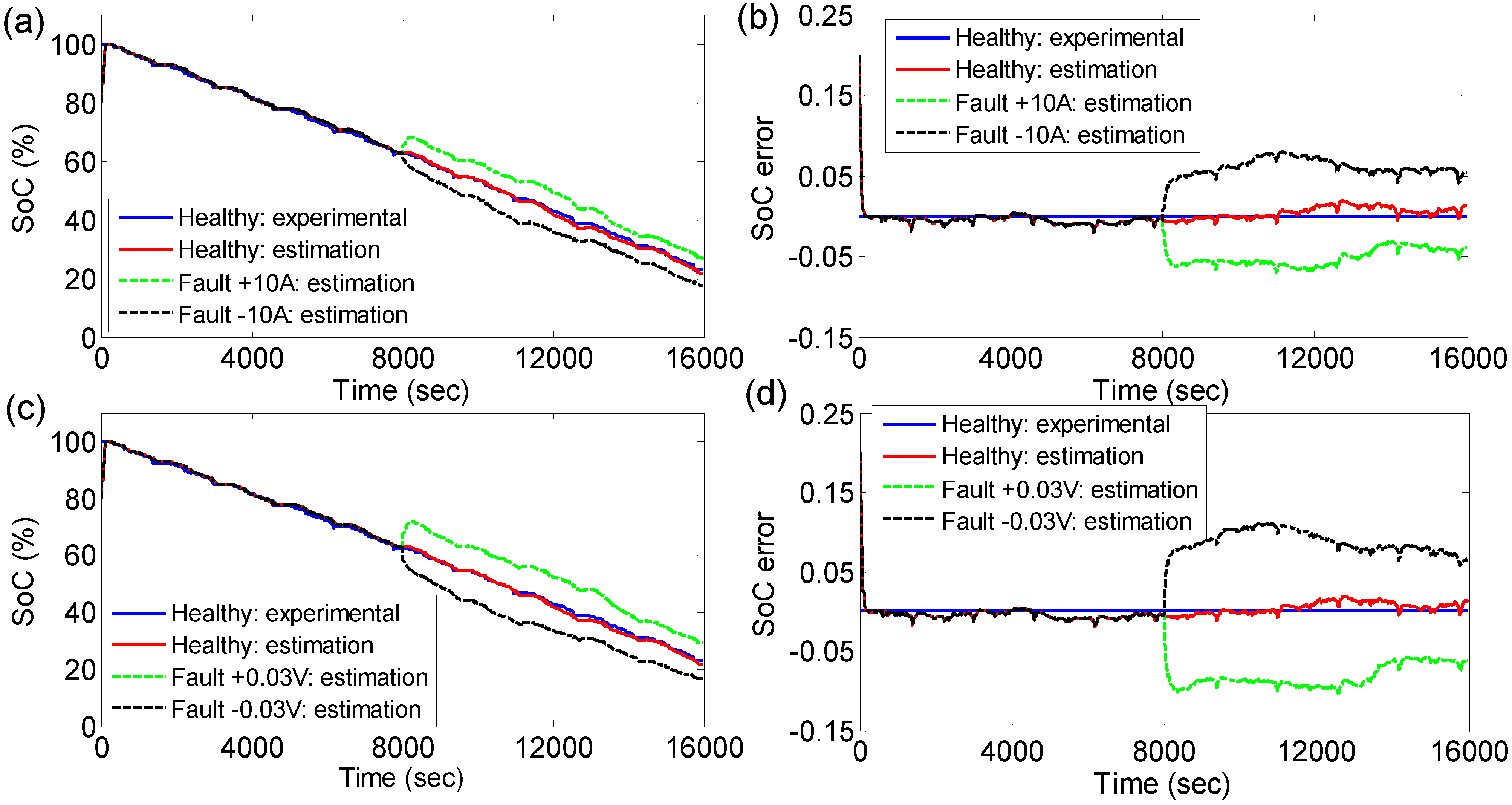
Figure 9.
Effects of sensor faults on battery SoC estimation under UDC test. (a) SoC estimation results in the current sensor healthy and faulty conditions; (b) SoC estimation errors in the current sensor healthy and faulty conditions; (c) SoC estimation results in the voltage sensor healthy and faulty conditions; (d) SoC estimation errors in the voltage sensor healthy and faulty conditions.

To prevent the battery from over-discharge, the lower limit of the battery SoC is taken as 20%. The current sensor fault with ±10 A bias was injected at the time 8000 s respectively. Figure 9a plots the experimental SoC in the sensor fault-free case, and estimation results under the current sensor fault-free and faulty conditions, while Figure 9b shows the SoC estimation errors. It can be found from Figure 9a that the computed SoC in BMS (EKF-estimated SoC) is around 30% at the time 16,000 s when the current sensor has a +10 A bias fault. Therefore, BMS will command to continually discharge the battery until SoC reaching around 20%, but in real life the battery has been at the lower limit. This will result in the battery suffering from over-discharge, accelerating the battery aging and decreasing the battery life. The computed SoC will prematurely reach 20% when the current sensor has a −10 A bias fault, and the battery cannot release the supposed energy. It can be found from Figure 9b that the estimation errors are out of the acceptable range 5% in the current sensor faulty cases.
Similar results could be found in Figure 9c,d when the voltage sensor with ±0.03 V fault was injected at the time of 8000 s. The battery may be over-discharged when the voltage sensor has a +0.03 V fault as shown in Figure 9c. It can be observed from Figure 9d that the estimation errors are around 10% under the voltage sensor faulty condition.
6. Experimental Diagnostic Evaluation
The purpose of this section is to validate the proposed diagnostic scheme. The proposed scheme is experimentally tested under the UDC and DST test conditions, including the recorded faulty current or voltage data. Due to the incorporated low-pass filter function into the measurement units, the large noise influences are eliminated. The errors of the installed Hall current and voltage sensor are less than 0.2% and 0.5%, respectively. The alarm threshold J is calibrated to be 300 (the alarm threshold J is calibrated through an extensive number of experimental tests under the fault-free and faulty conditions. To reduce the false alarm and missed detection due to the parameters variations in the changing environment, the experimental tests are performed in a controlled environment. This is also why the temperature is assumed to be constant. Besides, the threshold calibration needs to consider the maximum magnitudes of residuals under the fault-free tests).
6.1. Current Sensor Fault Detection
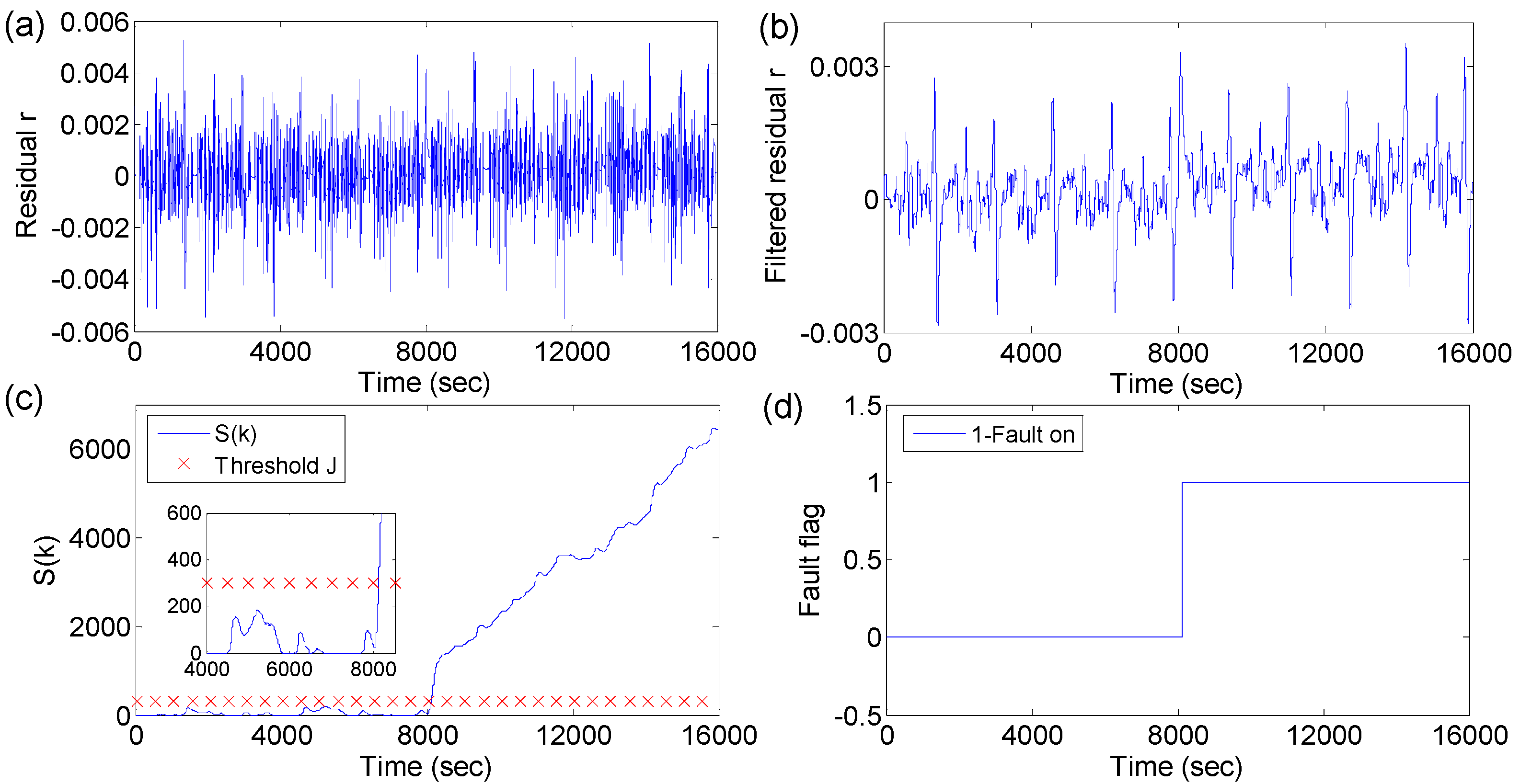
Different fault sizes and injection times are considered for the current sensor. For instance, the current sensor with a +3 A bias fault was injected into the UDC test at the time 8000 s, and the diagnostic results are shown in Figure 10. Figure 10a,b show the generated and filtered residual r respectively. It can be found from Figure 10a that the residual is non-zero in both the fault-free and faulty cases, and both show non-stationary behavior. Moreover, the behavior of the residual is similar before and after the fault injection. It is hard to tell from Figure 10a that a fault has occurred by using the constant thresholding approach. Actually, the mean of residual changes after the fault was injected at the time of 8000 s can be found from Figure 10b, but it is subtle. Through the CUSUM test as shown in Figure 10c, it can be found that S(k) continually increases from the time of 8000 s, and at the time of 8079 s, the alarm threshold J is crossed. This indicates the presence of a current sensor fault, and the detection signal is plotted in Figure 10d. There is a detection time delay of about 79 s, and this may be caused by the characteristics of the filter [23] and the defined threshold value. The possible explanation for the threshold is that it may be defined a little high, but there may be false alarms if the threshold is set lower. This tells us that there is a tradeoff between the false alarms and detection time. The detection time for the current sensor with different fault sizes and injection times under UDC tests are summarized in Table 1. It can be found that the larger the fault, the shorter the detection time. Besides, the detection time is correlated with the fault injection time because of the different dynamics at different times.
Figure 10.
Current sensor fault diagnostic results under UDC test. (a) Generated residual r; (b) Filtered residual r; (c) Residual evaluation result S(k) using CUSUM; (d) Detected current sensor fault.
Figure 10.
Current sensor fault diagnostic results under UDC test. (a) Generated residual r; (b) Filtered residual r; (c) Residual evaluation result S(k) using CUSUM; (d) Detected current sensor fault.


| Fault size | −1.5 A | +3 A | +5 A | +10 A |
|---|---|---|---|---|
| Injection time (7750 s–end) | 938 s | 68 s | 45 s | 29 s |
| Injection time (8000 s–end) | 997 s | 79 s | 67 s | 56 s |
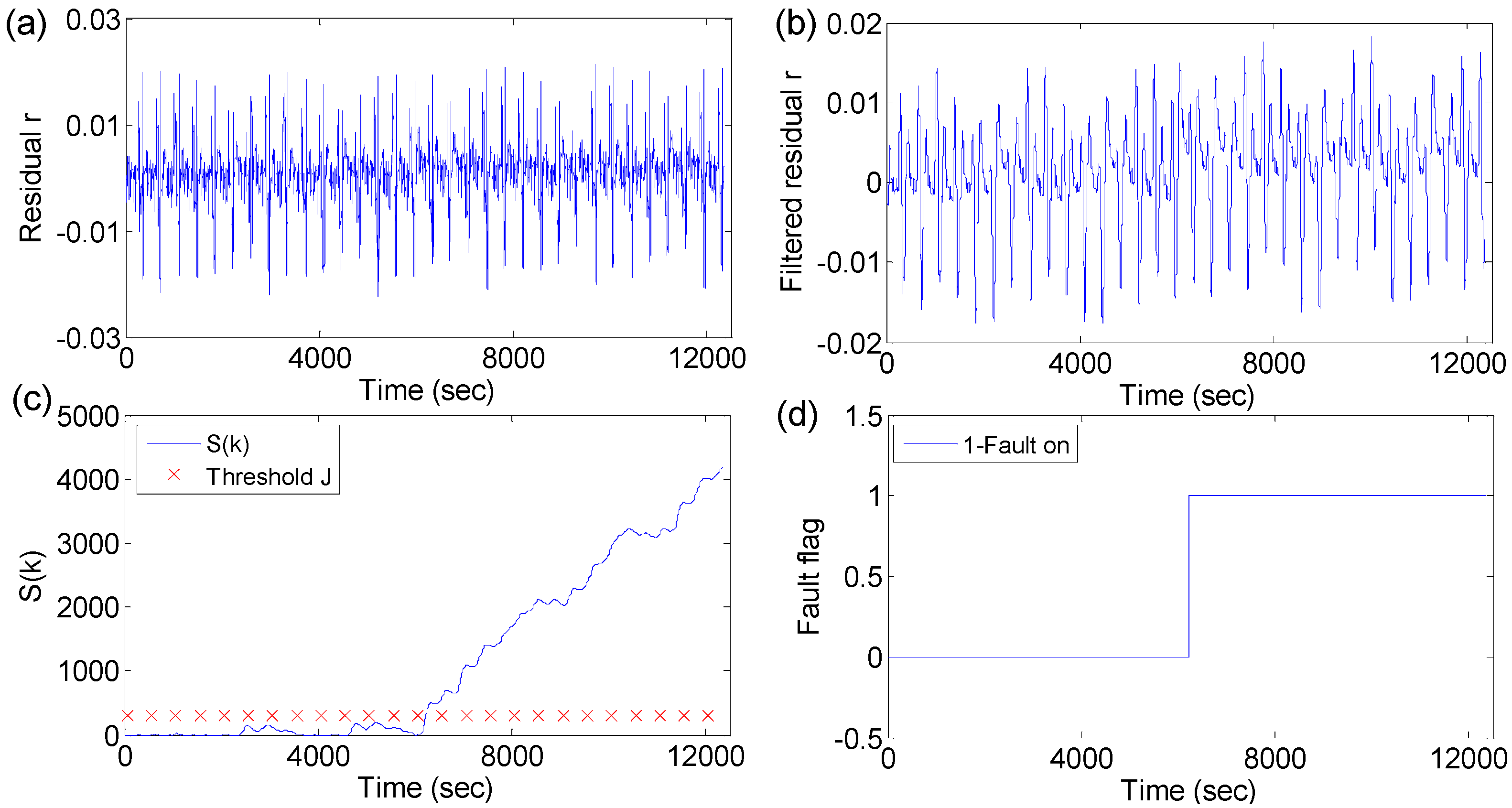
The DST tests were also performed to test the diagnostic performance of current sensor faults. Figure 11 shows the diagnostic results when a +3 A bias fault was injected at the time 6000 s, and the detection time is around 186 s. Through a number of experimental UDC and DST tests with different fault sizes and injection time, the maximum, minimum and mean detection time for the current sensor fault are obtained and summarized in Table 2. The detection times are reasonable and acceptable under different fault sizes.
Figure 11.
Current sensor fault diagnostic results under DST test. (a) Generated residual r; (b) Filtered residual r; (c) Residual evaluation result S(k) using CUSUM; (d) Detected current sensor fault.
Figure 11.
Current sensor fault diagnostic results under DST test. (a) Generated residual r; (b) Filtered residual r; (c) Residual evaluation result S(k) using CUSUM; (d) Detected current sensor fault.

| Fault size | −1.5 A | +3 A | +5 A | +10 A |
|---|---|---|---|---|
| Maximum (sec) | 962 | 189 | 56 | 35 |
| Minimum (sec) | 936 | 67 | 39 | 27 |
| Mean (sec) | 946 | 136 | 43 | 29 |
6.2. Voltage Sensor Fault Detection
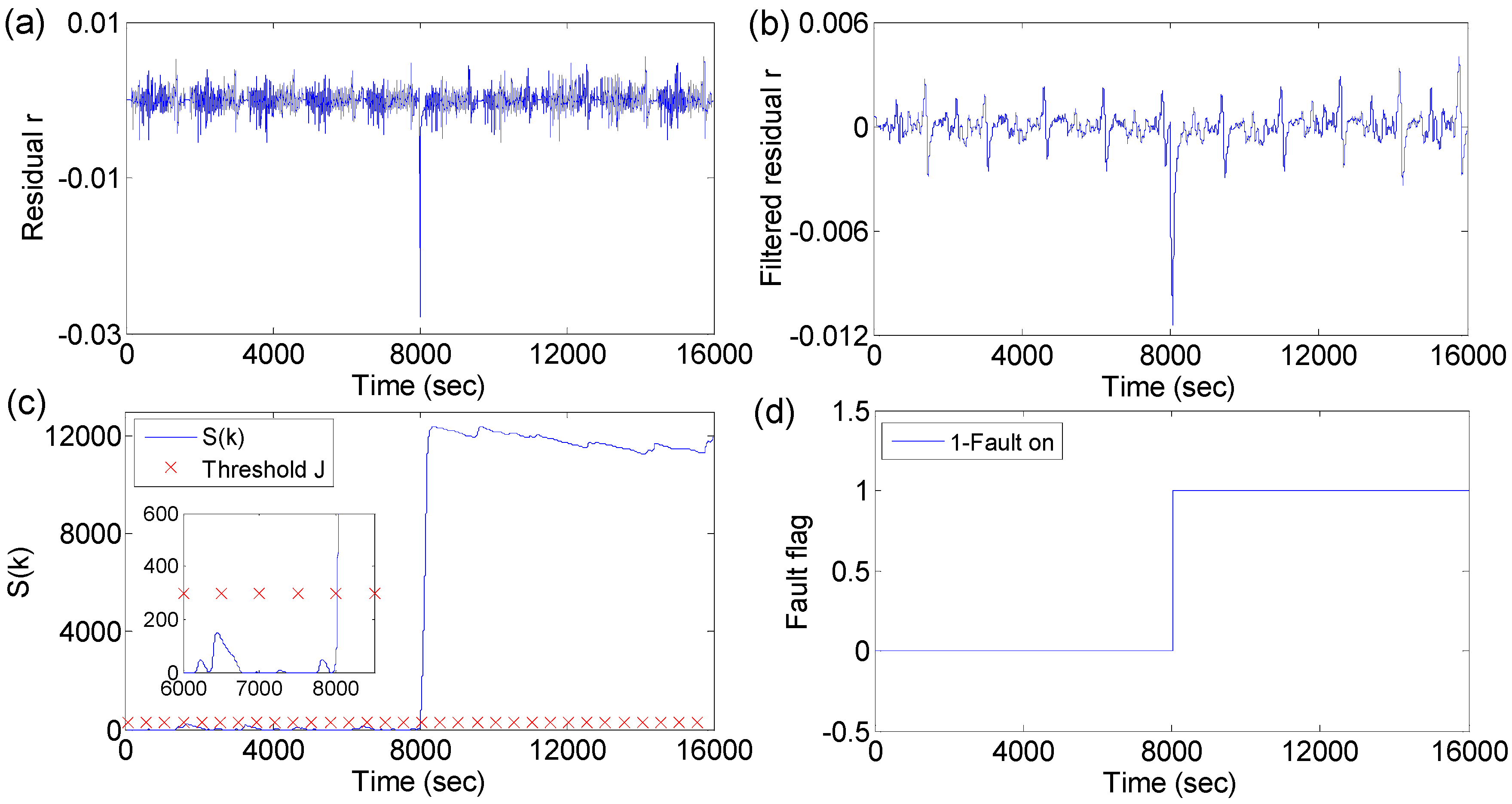
Similarly, the voltage sensor fault diagnostic performance is evaluated under the UDC and DST tests. Various fault sizes and injection times are considered for the voltage sensor. Taking the fault with −0.8% off-scaling injected into the UDC test at the time 8000 s as an example, the diagnostic results are plotted in Figure 12. Figure 12a,b show the generated and filtered residual r, respectively. It can be found from Figure 12a that the residual has a distinct drop around the time of 8000 s, and then the behavior of the residual quickly becomes similar than that before the fault injection. This distinct drop may be misunderstood as a disturbance. Through the CUSUM test as shown in Figure 12c, it can be observed that the threshold was exceeded at the time 8021 s, indicating the presence of the voltage sensor fault. The detected voltage sensor fault signal is plotted in Figure 12d. The detection time for the voltage sensor with different fault sizes and injection times under UDC tests are summarized in Table 3.
Figure 12.
Voltage sensor fault diagnostic results under UDC test. (a) Generated residual r; (b) Filtered residual r; (c) Residual evaluation result S(k) using CUSUM; (d) Detected voltage sensor fault.
Figure 12.
Voltage sensor fault diagnostic results under UDC test. (a) Generated residual r; (b) Filtered residual r; (c) Residual evaluation result S(k) using CUSUM; (d) Detected voltage sensor fault.

| Fault size | −0.8% | +1% | +1.5% | +2% |
|---|---|---|---|---|
| Injection time (7750 s–end) | 39 s | 16 s | 10 s | 8 s |
| Injection time (8000 s–end) | 23 s | 20 s | 16 s | 10 s |
The example of DST tests for voltage sensor fault with −0.8% off scaling injected at the time 6000 s is shown in Figure 13. The same fault size but a different fault injection time is considered. The detection time is around 55 s. Finally, the maximum, minimum and mean detection time for the voltage sensor fault under a number of UDC and DST tests are summarized in Table 4. Compared to the current sensor fault detection time in Table 2, the detection time for voltage sensor fault is relatively shorter. This tells us that the residual is much more sensitive to voltage sensor faults than current sensor faults. It is reasonable since the residual is generated through the voltage signal.
Figure 13.
Voltage sensor fault diagnostic results under DST test. (a) Generated residual r; (b) Filtered residual r; (c) Residual evaluation result S(k) using CUSUM; (d) Detected voltage sensor fault.
Figure 13.
Voltage sensor fault diagnostic results under DST test. (a) Generated residual r; (b) Filtered residual r; (c) Residual evaluation result S(k) using CUSUM; (d) Detected voltage sensor fault.

| Fault size | −0.8% | +1% | +1.5% | +2% |
|---|---|---|---|---|
| Maximum (sec) | 56 | 39 | 25 | 17 |
| Minimum (sec) | 23 | 19 | 13 | 8 |
| Mean (sec) | 36 | 26 | 17 | 11 |
7. Conclusions
This paper presents a systematic model-based diagnostic scheme for a lithium-ion battery cell to determine the presence of the current or voltage sensor faults. The following conclusions may be put forth:
- (1)
- Based on the second order equivalent circuit model, EKF is used to estimate the battery terminal voltage to generate a residual carrying the fault information. The residual is then evaluated by a statistical CUSUM test to make a reliable diagnostic decision.
- (2)
- To highlight the importance of sensor fault diagnosis, the effects of current or voltage sensor faults on battery SoC estimation are analyzed. The results show the battery may be over-discharged in the faulty sensor cases.
- (3)
- The proposed diagnostic scheme is experimentally validated under the UDC and DST driving cycles. Different fault sizes and injection times are considered to evaluate the fault detection performance. The results show current or voltage sensor faults could be accurately detected in a reasonable time.
Acknowledgments
This work was supported by National High Technology Research and Development Program of China (2013BAG05B00) in part, National Natural Science Foundation of China (51276022) in part, Program for New Century Excellent Talents in University (NCET-11-0785) in part, and the Higher school discipline innovation intelligence plan (“111”plan) in part.
Author Contributions
All authors contributed to this work in collaboration. Zhentong Liu validated the model and implemented the proposed diagnostic scheme, and Hongwen He provided substantial help with the experimental setup and the battery test schedule.
Conflicts of Interest
The authors declare no conflict of interest.
References
- Striebel, K.; Shim, J.; Sierra, A.; Yang, H.; Song, X.; Kostecki, R.; McCarthy, K. The development of low cost LiFePO4-based high power lithium-ion batteries. J. Power Sources 2005, 146, 33–38. [Google Scholar] [CrossRef]
- Lu, L.; Han, X.; Li, J.; Hua, J.; Ouyang, M. A review on the key issues for lithium-ion battery management in electric vehicles. J. Power Sources 2013, 226, 272–288. [Google Scholar] [CrossRef]
- Mikolajczak, C.; Kahn, M.; White, K.; Thomas, L.R. Lithium-Ion Batteries Hazard and Use Assessment; Springer: New York, NY, USA, 2011. [Google Scholar]
- Barré, A.; Deguilhem, B.; Grolleau, S.; Gérard, M.; Suard, F.; Riu, D. A review on lithium-ion battery ageing mechanisms and estimations for automotive applications. J. Power Sources 2013, 241, 680–689. [Google Scholar] [CrossRef]
- Balaban, E.; Saxena, A.; Bansal, P.; Goebel, K.F.; Curran, S. Modeling, detection, and disambiguation of sensor faults for aerospace applications. IEEE Sens. J. 2009, 9, 1907–1917. [Google Scholar] [CrossRef]
- Plett, G.L. Extended Kalman filtering for battery management systems of LiPB-based HEV battery packs—Part 3. State and parameter estimation. J. Power Sources 2004, 134, 277–292. [Google Scholar] [CrossRef]
- Blanke, M.; Kinnaert, M.; Lunze, J.; Staroswiecki, M. Diagnosis and Fault-Tolerant Control, 2nd ed.; Springer: New York, NY, USA, 2006. [Google Scholar]
- Venkatasubramanian, V.; Rengaswamy, R.; Yin, K.; Kavuri, S. A review of process fault detection and diagnosis—Part II: Qualitative models and search strategies. Comput. Chem. Eng. 2003, 27, 313–326. [Google Scholar] [CrossRef]
- Isermann, R. Model-based fault-detection and diagnosis—Status and applications. Annu. Rev. Control 2005, 29, 71–85. [Google Scholar] [CrossRef]
- Chen, W.; Chen, W.T.; Saif, M.; Li, M.F.; Wu, H. Simultaneous Fault Isolation and Estimation of Lithium-Ion Batteries via Synthesized Design of Luenberger and Learning Observers. IEEE Trans. Control Syst. Technol. 2014, 22, 290–298. [Google Scholar] [CrossRef]
- Marcicki, J.; Onori, S.; Rizzoni, G. Nonlinear fault detection and isolation for a lithium-ion battery management system. In Proceedings of the ASME 2010 Dynamic System and Control Conference, Cambridge, MA, USA, 12–15 September 2010.
- Singh, A.; Izadian, A.; Anwar, S. Adaptive Nonlinear Model-Based Fault Diagnosis of Li-ion Batteries. IEEE Trans. Ind. Electron. 2015, 62, 1002–1011. [Google Scholar]
- Hajiyev, C. Innovation Approach Based Sensor FDI in LEO Satellite Attitude Determination and Control System. In Kalman Filter: Recent Advances and Application; 1-Tech Education and Publishing KG: Vienna, Austria, 2009; pp. 347–374. [Google Scholar]
- Shang, L.; Liu, G. Sensor and Actuator Fault Detection and Isolation for a High Performance Aircraft Engine Bleed Air Temperature Control System. IEEE Trans. Control Syst. Technol. 2011, 19, 1260–1268. [Google Scholar] [CrossRef]
- An, L.; Sepehri, N. Hydraulic actuator circuit fault detection using extended Kalman filter. In Proceedings of the 2003 American Control Conference, Denver, CO, USA, 4–6 June 2003; Volume 5, pp. 4261–4266.
- Foo, G.H.; Zhang, X.; Vilathgamuwa, D.M. A Sensor Fault Detection and Isolation Method in Interior Permanent-Magnet Synchronous Motor Drives Based on an Extended Kalman Filter. IEEE Trans. Ind. Electron. 2013, 60, 3485–3495. [Google Scholar] [CrossRef]
- Diao, S.; Makni, Z.; Bisson, J.F.; Diallo, D.; Marchand, C. Sensor Fault Diagnosis for Improving the Availability of Electrical Drives. In Proceedings of the IECON 2013—39th Annual Conference of the IEEE Industrial Electronics Society, Vienna, Austria, 10–13 November 2013; pp. 3108–3113.
- Hu, X.; Li, S.; Peng, H. A comparative study of equivalent circuit models for Li-ion batteries. J. Power Sources 2012, 198, 359–367. [Google Scholar] [CrossRef]
- Ioannou, P.A.; Sun, J. Robust Adaptive Control; Dover Publications: Mineola, NY, USA, 1996. [Google Scholar]
- Simon, D. Optimal State Estimation Kalman, H Infinite, and Nonlinear Approaches; Wiley-Interscience: Hoboken, NJ, USA, 2006. [Google Scholar]
- Rizzoni, G. Statistical inference methods for residual analysis and change detection. In The Ohio Sate University Lecture; Ohio State University: Columbus, OH, USA, 2014. [Google Scholar]
- The Idaho National Laboratory. Battery Test Manual for Plug-In Hybrid Electric Vehicles; Idaho National Laboratory: Idaho Falls, ID, USA, 2010. [Google Scholar]
- Redinbo, G.R. Decoding real-number convolutional codes: Change detection, Kalman estimation. IEEE Trans. Inf. Theory 1997, 43, 1864–1876. [Google Scholar] [CrossRef]
© 2015 by the authors; licensee MDPI, Basel, Switzerland. This article is an open access article distributed under the terms and conditions of the Creative Commons Attribution license (http://creativecommons.org/licenses/by/4.0/).
Share and Cite
MDPI and ACS Style
Liu, Z.; He, H. Model-based Sensor Fault Diagnosis of a Lithium-ion Battery in Electric Vehicles. Energies 2015, 8, 6509-6527. https://doi.org/10.3390/en8076509
AMA Style
Liu Z, He H. Model-based Sensor Fault Diagnosis of a Lithium-ion Battery in Electric Vehicles. Energies. 2015; 8(7):6509-6527. https://doi.org/10.3390/en8076509
Chicago/Turabian StyleLiu, Zhentong, and Hongwen He. 2015. "Model-based Sensor Fault Diagnosis of a Lithium-ion Battery in Electric Vehicles" Energies 8, no. 7: 6509-6527. https://doi.org/10.3390/en8076509