Thermal Analysis of a Novel Cylindrical Transverse-Flux Permanent-Magnet Linear Machine

Abstract

This paper presents a novel staggered-teeth cylindrical transverse-flux permanent-magnet linear machine (TFPMLM), which aims to improve the power factor and force density. Due to the compact structure and high performance requirement, thermal problems should be seriously considered. The three-dimensional (3-D) temperature field model is established. The determination of convection heat transfer coefficients is discussed. Equivalent thermal conductivities of stator core and winding are given to simplify the analysis. With the thermal effect of the adhesive coatings among permanent magnets (PMs) and mover yoke taken into account, the temperature field distribution and variation rules of the TFPMLM are obtained using the finite volume method (FVM). The influences of slot filling factor and air flow velocity on the temperature field distribution are analyzed. It is found that the hottest spot of the TFPMLM appears in the middle of the end winding; and there is no risk of demagnetization for PMs.

1. Introduction

In the past decade, transverse-flux permanent-magnet linear machine (TFPMLM) has been widely employed in the applications of electrical power generation [1,2,3,4,5], magnetic levitation [6,7], electromagnetic launcher [8,9], etc. [10]. Many scholars have been dedicated to the analysis, design and optimization of TFPMLM using the approaches of equivalent magnetic circuit network (EMCN) [11,12], finite element method (FEA) [1,2], modern intelligent algorithms [10,13].

However, the TFPMLM generally has the disadvantages of low power factor and complex structure leading to difficult manufacturability. A novel staggered-teeth TFPMLM is proposed in order to solve the problems of high flux leakage and low power factor existing in the conventional TFPMLM [14,15,16]. For the staggered-teeth TFPMLM, the three phases can be arranged in axial direction or circumferential direction, and cylindrical topologies are particularly competitive for free-piston energy converter applications. In [15], optimizations of the leakage factor for two staggered-teeth topologies and the performance comparison between them are carried out; in addition, the methods to improve force density and power factor for the staggered-teeth TFPMLM are researched. In [16], a comprehensive analysis of flux leakage, no-load and load characteristics with different axial thicknesses of stator core is made; furthermore, a cut-tip stator tooth is adopted to cripple the thrust ripple and increase the power factor. Compared with the TFPMLM employing soft magnetic composite (SMC) to achieve the complex structure and three-dimensional (3-D) flux path, the stator core of staggered-teeth TFPMLM is laminated by electrical-steel sheets, which results in a relatively simple manufacturing process and high reliability [17,18].

Due to the compact structure and high performance requirement, thermal problems should be seriously considered. This paper focuses on the thermal analysis of circumferential three-phase topology of the staggered-teeth TFPMLM. A 3-D temperature field model is established and corresponding boundary conditions, especially the determination of convection heat transfer coefficients, are discussed. A comprehensive research on temperature rise is carried out. The influences of air flow velocity and slot filling factor on the temperature field distribution are analyzed.

2. Transverse-Flux Permanent-Magnet Linear Machine (TFPMLM) Temperature Field Model

2.1. Structure of the Transverse-Flux Permanent-Magnet Linear Machine (TFPMLM)

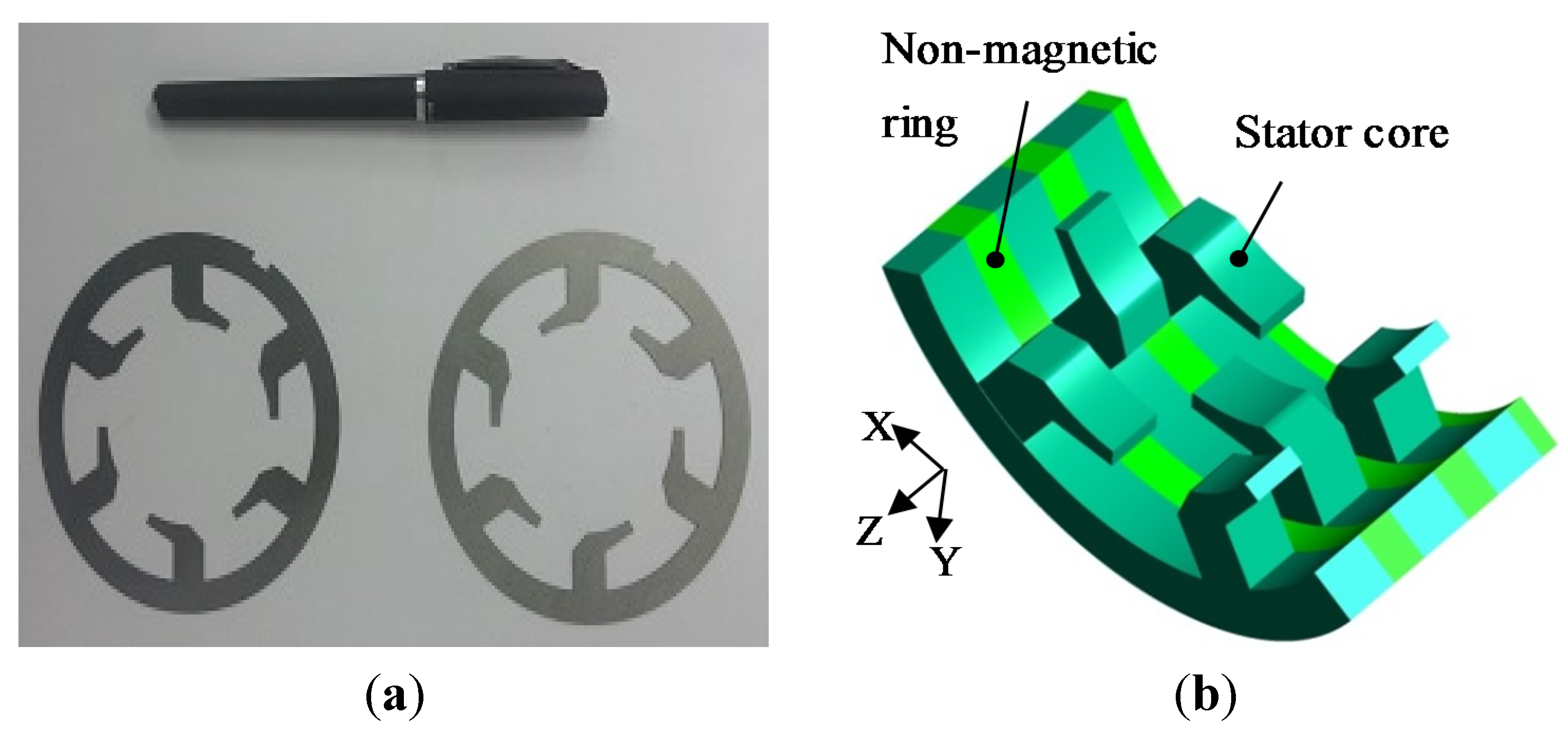
The schematic diagram of the staggered-teeth TFPMLM prototype is shown in Figure 1. The machine is self-cooled. For every pole pair, the stacked stator core is composed of two types of laminations, as shown in Figure 2; two axially adjacent stacked stator cores are separated by a non-magnetic ring. By employing the staggered teeth, the axial pole-to-pole armature flux leakage can be reduced dramatically. There are six stator teeth along the circumferential direction. Each coil is wound around one tooth, and two adjacent coils in series form one phase winding. Six coils are evenly divided into three phases.

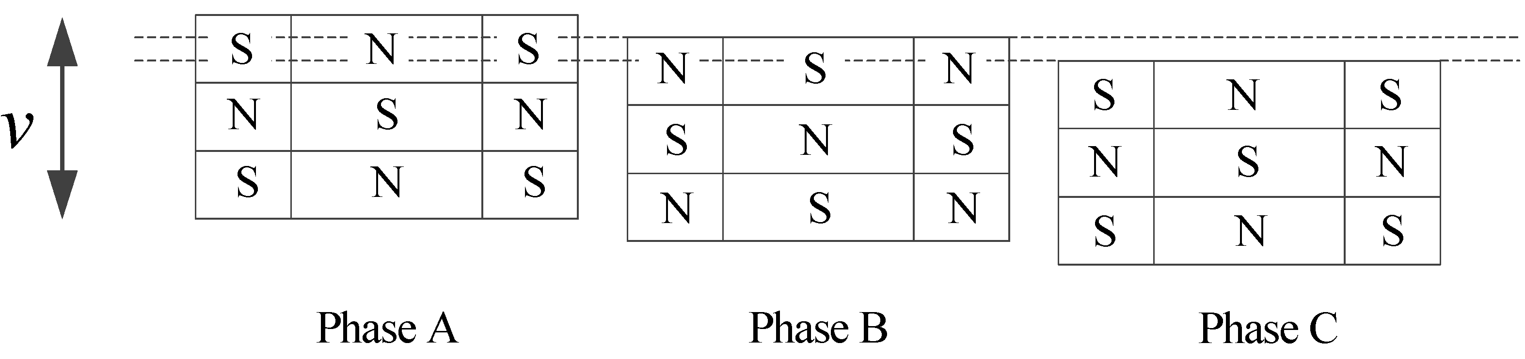
The permanent magnets (PMs) of two adjacent phases are arranged by 2/3 pole pitch displacement in the axial direction. The arrangement of PMs are shown in Figure 3, where v refers to the motion direction. On the basis of the optimization with the targets of minimizing the flux leakage and maximizing the force density [14,15,16], an optimum design for the TFPMLM is obtained, and the basic parameters are listed in Table 1.

Figure 1. Schematic diagram of the transverse-flux permanent-magnet linear machine (TFPMLM). PM: permanent magnet.

Figure 1. Schematic diagram of the transverse-flux permanent-magnet linear machine (TFPMLM). PM: permanent magnet.

Figure 2. Stator lamination of the TFPMLM: (a) lamination; and (b) model of the stator core.

Figure 2. Stator lamination of the TFPMLM: (a) lamination; and (b) model of the stator core.

Figure 3. Arrangement of PMs.

Figure 3. Arrangement of PMs.

Table 1. Basic parameters of the transverse-flux permanent-magnet linear machine (TFPMLM).

Parameters	Value	Parameters	Value
Rated power (W)	500	Rated current (A)	8
Power factor	0.71	Pole-arc coefficient	1
PM	NdFe35	Thickness of PM (mm)	4
Casing outer diameter (mm)	120	Stator outer diameter (mm)	100
Stator inner diameter (mm)	54	Mover outer diameter (mm)	52

Table 1. Basic parameters of the transverse-flux permanent-magnet linear machine (TFPMLM).

Parameters	Value	Parameters	Value
Rated power (W)	500	Rated current (A)	8
Power factor	0.71	Pole-arc coefficient	1
PM	NdFe35	Thickness of PM (mm)	4
Casing outer diameter (mm)	120	Stator outer diameter (mm)	100
Stator inner diameter (mm)	54	Mover outer diameter (mm)	52

2.2. Physical Model

The process of temperature field analysis involves electromagnetic, fluid mechanics and heat transfer theory, which is extraordinarily complicated [19,20,21,22,23,24]. The temperature field model is established. The solved region is minimized to reduce computational cost, and some secondary factors which have little impact on the heat generation and cooling effect are simplified. Some assumptions are made as follows:

(1) The central cross section in the axial direction is the symmetry plane according to the structure of the TFPMLM prototype, so the heat generation and cooling condition are symmetrical in the two regions divided by the central cross section.

(2) Heat generation and cooling condition are also considered symmetrical for the three circumferential sectorial regions which correspond to the three phases.

(3) The influences of mechanical loss and shaft are neglected.

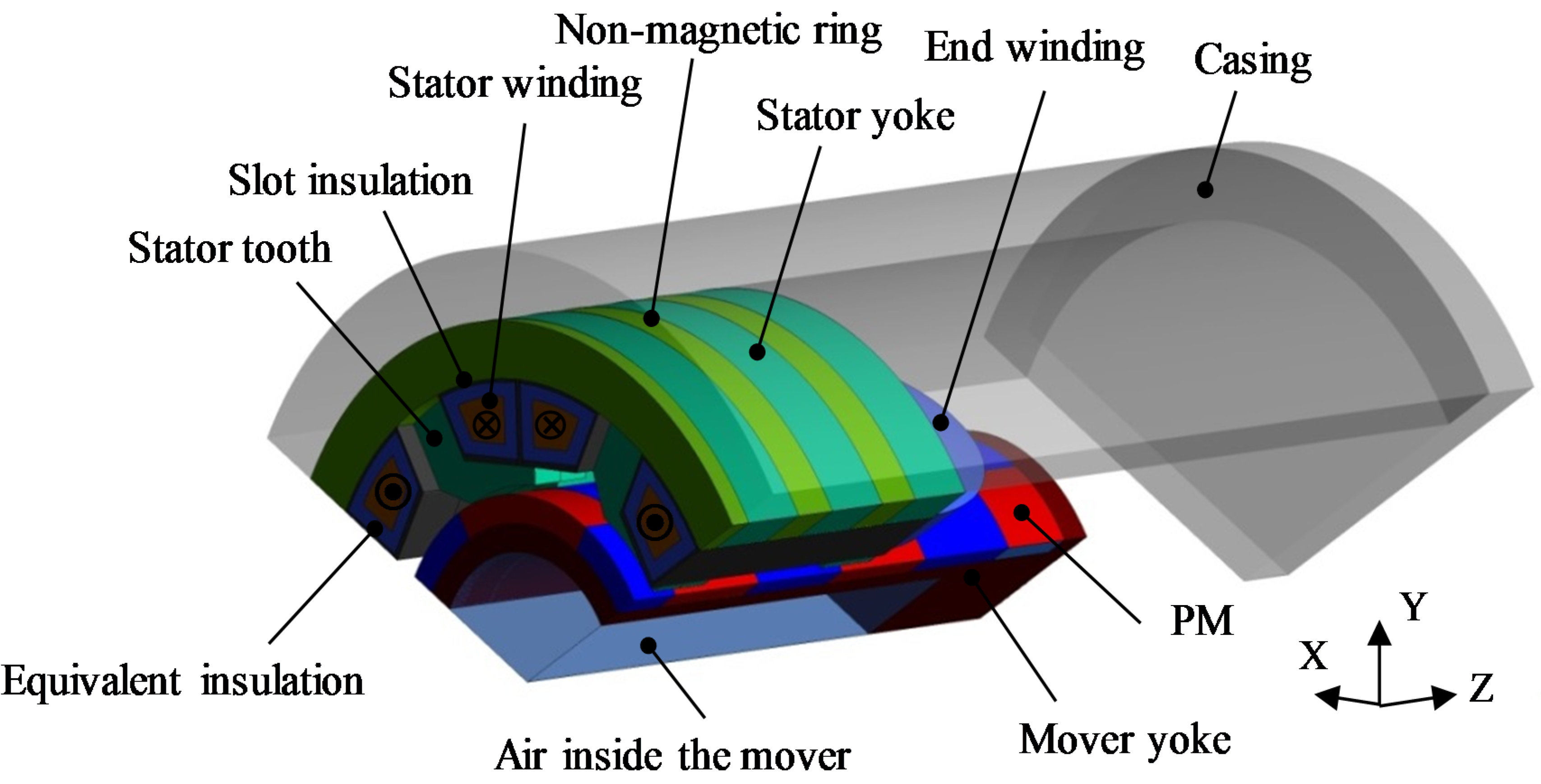
Based on the aforementioned assumption, a 3-D temperature field model of the TFPMLM is established in this paper. The model covers half length of the prototype in the axial direction and one third in the circumferential direction, as illustrated in Figure 4. It includes stator winding, stator yoke, stator tooth, slot insulation, equivalent insulation, casing, mover yoke, PM, and air inside the mover. The ☉ and ⊗ indicate the direction of the winding.

Figure 4. Physical model of the TFPMLM temperature field.

Figure 4. Physical model of the TFPMLM temperature field.

The air inside the mover, which is an enclosed area, can be regarded as relatively static to the mover during the operation of the TFPMLM. The heat produced by the eddy current loss of the mover yoke conducts to the air by conduction heat transfer; consequently, the air inside the mover is modeled and treated as a solid component. Due to staggered and separated arrangement of PMs, the eddy current loss of each piece of PM is different. In order to consider its influence on temperature field distribution of the mover, the PMs are modeled separately along the axial and circumferential direction.

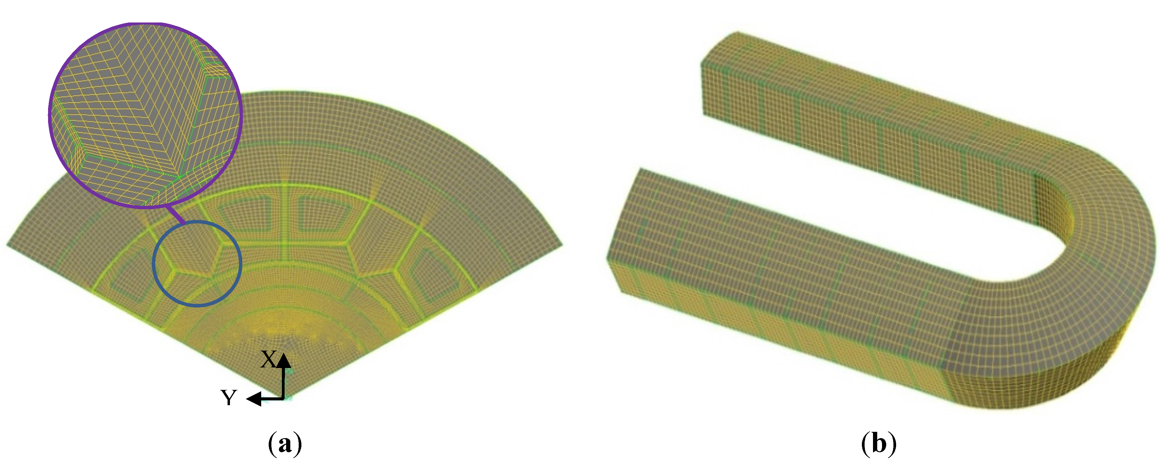
Meshing quality has a significant influence on the precision of FVM analysis. The 3-D TFPMLM physical model is meshed using hexahedron elements, in total 1,749,360 nodes and 1,532,098 elements. Small size region, such as slot insulation, and focused region, such as stator winding, are meshed smoothly and intensively, as shown in Figure 5.

Figure 5. Meshing of the physical model: (a) local view; and (b) stator winding.

Figure 5. Meshing of the physical model: (a) local view; and (b) stator winding.

2.3. Mathematical Model and Boundary Conditions

Based on the heat transfer theory, a mathematical model for 3-D temperature field of the TFPMLM is shown [25]:

$$\frac{\partial T}{\partial x}\left({\text{λ}}_x\frac{\partial T}{\partial x}\right)+\frac{\partial T}{\partial y}\left({\text{λ}}_y\frac{\partial T}{\partial y}\right)+\frac{\partial T}{\partial z}\left({\text{λ}}_z\frac{\partial T}{\partial z}\right)+\dot{q}=0$$

(1)

where T is temperature; λ_x, λ_y, λ_z are thermal conductivities in x-, y- and z- directions, respectively; $\dot{q}$ is heat generated per unit volume.

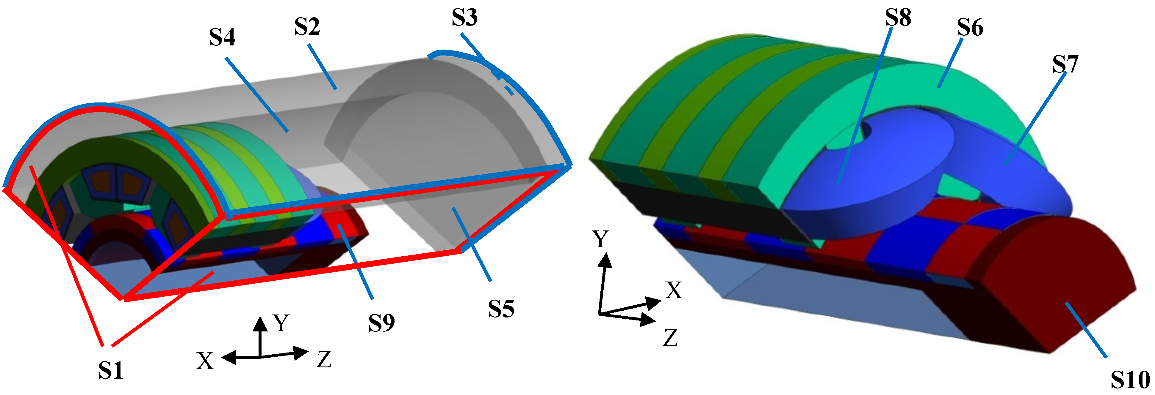
The corresponding boundary conditions are required to determine the unique solution of this thermal issue. Figure 6 illustrates the boundary conditions to be determined. According to the basic assumptions and operating condition of the TFPMLM, the boundary conditions of the TFPMLM can be determined as follows:

(1) The central cross section in axial direction and the two cut planes in circumferential direction are adiabatic surfaces (S1, red area); which satisfy the Neumann boundary condition as:

$${-{\text{λ}}_n\frac{\partial T}{\partial n}|}_{\text{S1}}=0$$

(2)

where λ_n is thermal conductivity in normal direction of the surface.

(2) The surfaces which directly contact the cooling air satisfy the Robin boundary condition as Equation (3):

$${-{\text{λ}}_n\frac{\partial T}{\partial n}|}_{\text{S2-S10}}=h(T-T_{\text{f}})$$

(3)

where h is convection heat transfer coefficient; T_f is temperature of free stream. The involved surfaces include the outer surfaces of casing and end cap S2/S3 (blue area), inner surface of casing S4, inner surface of end cap S5, outer surface of stator core in end region S6, surface of end winding S7/S8, surface of PMs S9, outer surface of mover S10. The convection heat transfer coefficients of each surface are discussed in Section 3 in detail.

(3) The ambient temperature is 20 °C.

Figure 6. Boundary of the TFPMLM temperature field model: S2: outer surface of casing; S3: outer surface of end cap; S4: inner surface of casing; S5: inner surface of end cap, S6: outer surface of stator core in end region; S7: vertical outer surface of end winding; S8: horizontal outer surface of end winding; S9: outer surface of PMs; and S10: outer surface of mover.

Figure 6. Boundary of the TFPMLM temperature field model: S2: outer surface of casing; S3: outer surface of end cap; S4: inner surface of casing; S5: inner surface of end cap, S6: outer surface of stator core in end region; S7: vertical outer surface of end winding; S8: horizontal outer surface of end winding; S9: outer surface of PMs; and S10: outer surface of mover.

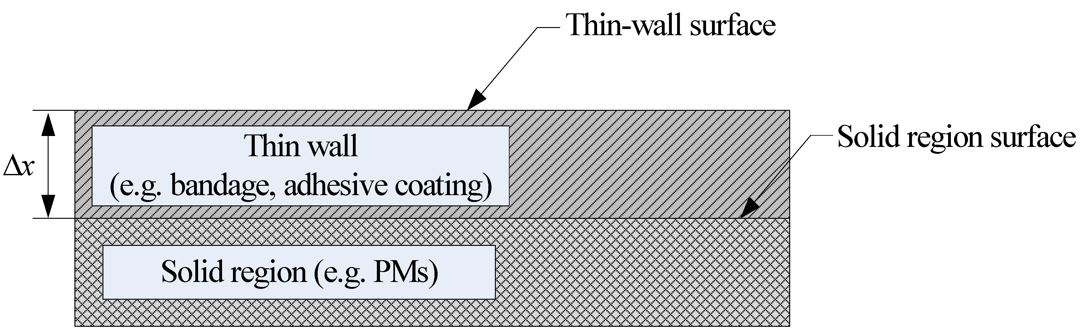
The PMs are glued to the mover yoke as well as to other adjacent PMs, and are also bound to mover yoke through a bandage. The thermal conductivities of adhesive coating and bandage are comparatively smaller than that of PM, thus having a certain influence on heat transfer of the PMs and mover yoke. However, their thicknesses within the range of 0.2 mm to 0.4 mm are too thin to model in the thermal analysis. A thin-wall thermal resistance boundary is adopted to simulate the thermal influence of the adhesive coating and bandage [26]. Their thicknesses and materials need to be specified, thus obtaining a thermal resistance per unit area of the thin-wall, which is given as:

$$R_{\text{p}}=\mathrm{\Delta }x/k$$

(4)

where $\mathrm{\Delta }x$ is the thickness of the thin wall; k is thermal conductivity of the thin wall. The boundary condition specified originally on the surface of the solid region is transferred to the surface of the thin wall, as illustrated in Figure 7. A one-dimensional steady heat conduction equation is used to compute the temperature gradient inside the thin-wall, and it is assumed that the heat conduction is only along the radial direction in the thin wall.

Figure 7. Schematic diagram of the thin-wall thermal resistance boundary.

Figure 7. Schematic diagram of the thin-wall thermal resistance boundary.

3. Determination of the Critical Thermal Parameters

3.1. Convection Heat Transfer Coefficient

The heat transfer coefficient is a key factor in the precise simulation of temperature field distribution. Heat transfer coefficient has a dependence on the thermal properties of the fluid (viscosity, thermal conductivity, specific heat, density), flow velocity of the fluid, and characteristic dimension of the geometry. Accordingly, predicting the values of convection heat transfer coefficient is a complicated and crucial process, particularly for the complex situations in an electric machine. This section presents the determinations of the convection heat transfer coefficients for those surfaces satisfying Robin boundary condition.

3.1.1. Heat Transfer Coefficients for Forced Convection Surfaces

The air confined in the casing is forced to move due to the reciprocating motion of the mover, and conducts forced convection heat transfer with the surfaces S4, S5, S9, and S10. The empirical correlations in the forced convection system are used to estimate the heat transfer coefficients of foregoing surfaces [25,27,28,29].

The judgement of flow condition of forced flow air is the essential step to determine the proper empirical correlations to adopt. Reynolds number is widely used as a criterion for laminar and turbulent flow:

$$Re=\frac{ul}{\nu }$$

(5)

where Re is Reynolds number; u is air flow velocity; l is characteristic dimension of geometry; v is kinematic viscosity.

For Re > 2300, the forced-flow air is in transition or turbulence, and the heat transfer coefficients for S4 and S9 are calculated according to Equation (6) developed by Dittus and Boelter for forced convection heat transfer in pipe and tube flow [25]:

$$Nu=0.023R{e}^{0.8}P{r}^{0.4}$$

(6)

Where Pr is Prandtl Number, a dimensionless parameter associated with kinematic viscosity v and thermal diffusivity α.

For Re < 2300, the forced-flow air is laminar, and the Nusselt number, which depends on the ratio of inner diameter d_i and outer diameter d_o of an annular tube, is adopted to estimate the heat transfer coefficients of the surfaces S4 and S9. Table 2 shows the Nusselt number at inner wall and outer wall with different ratios of d_i and d_o. The surfaces S4 and S9 are analogous to the outer wall and inner wall of an annular tube, respectively, and the ratio of d_i and d_o equals 0.52. The Nusselt number at S4 and S9 are determined as 5.05 and 6.14 by parabola interpolation.

In terms of the surfaces S5 and S10 which are vertical in the casing, their heat transfer coefficients can be estimated by the empirical correlation for flow across vertical plate, which is presented as:

$$Nu=0.228R{e}^{0.731}P{r}^{1/3}$$

(7)

Table 2. Nusselt number of laminar flow in annular tube.

di/do	Nu
	Inner wall	Outer wall
0	/	4.364
0.05	17.81	4.792
0.10	11.91	4.834
0.20	8.499	4.833
0.40	6.583	4.979
0.60	5.912	5.099
0.80	5.580	5.240
1.00	5.385	5.385

Table 2. Nusselt number of laminar flow in annular tube.

di/do	Nu
	Inner wall	Outer wall
0	/	4.364
0.05	17.81	4.792
0.10	11.91	4.834
0.20	8.499	4.833
0.40	6.583	4.979
0.60	5.912	5.099
0.80	5.580	5.240
1.00	5.385	5.385

3.1.2. Heat Transfer Coefficients for Free Convection Surfaces

The casing outer surface S2 and the end cap outer surface S3 of the TFPMLM are exposed to ambient air without an external source of motion, thus the surfaces S2 and S3 can be typically treated as free convection heat transfer surfaces. The flow velocity of the air near the stator end winding is approximately zero, thus the outer surface of the stator core in end region S6, the vertical outer surface of end winding S7, and the horizontal outer surface of end winding S8 are assumed to in the free convection heat transfer environment.

The empirical correlations for the free convection system are also strongly dependent on the flow condition of the fluid. As the function of Reynolds number in forced convection system, the Grashof number Gr is the primary criterion for the transition from laminar to turbulent flow in the free convection system, which is defined as:

$$Gr=\frac{g{\text{α}}_{\text{V}}(T_{\text{w}}-T_{\text{f}})l^3}{{\nu }^2}$$

(8)

where g is acceleration of gravity; α_V is coefficient of thermal expansion; T_w is wall temperature.

Equation (9) with a variety of constant C and n for different circumstances can be used to estimate the heat transfer coefficient in free convection system:

$$Nu=C{(GrPr)}^n$$

(9)

where Pr is the Prandtl number. The constant C and n depending on the geometry characteristic as well as the Grashof number are indicated in Table 3.

The Grashof number of the air in the casing and in the ambient conditions are both estimated to be less than 10⁸. For either vertical planes or horizontal cylinders, the flow condition of air is laminar flow according to Table 3. Thus for the surfaces S2 and S8, the constant C = 0.48, n = 0.25; for the surfaces S3, S6 and S7, the constant C = 0.59, n = 0.25.

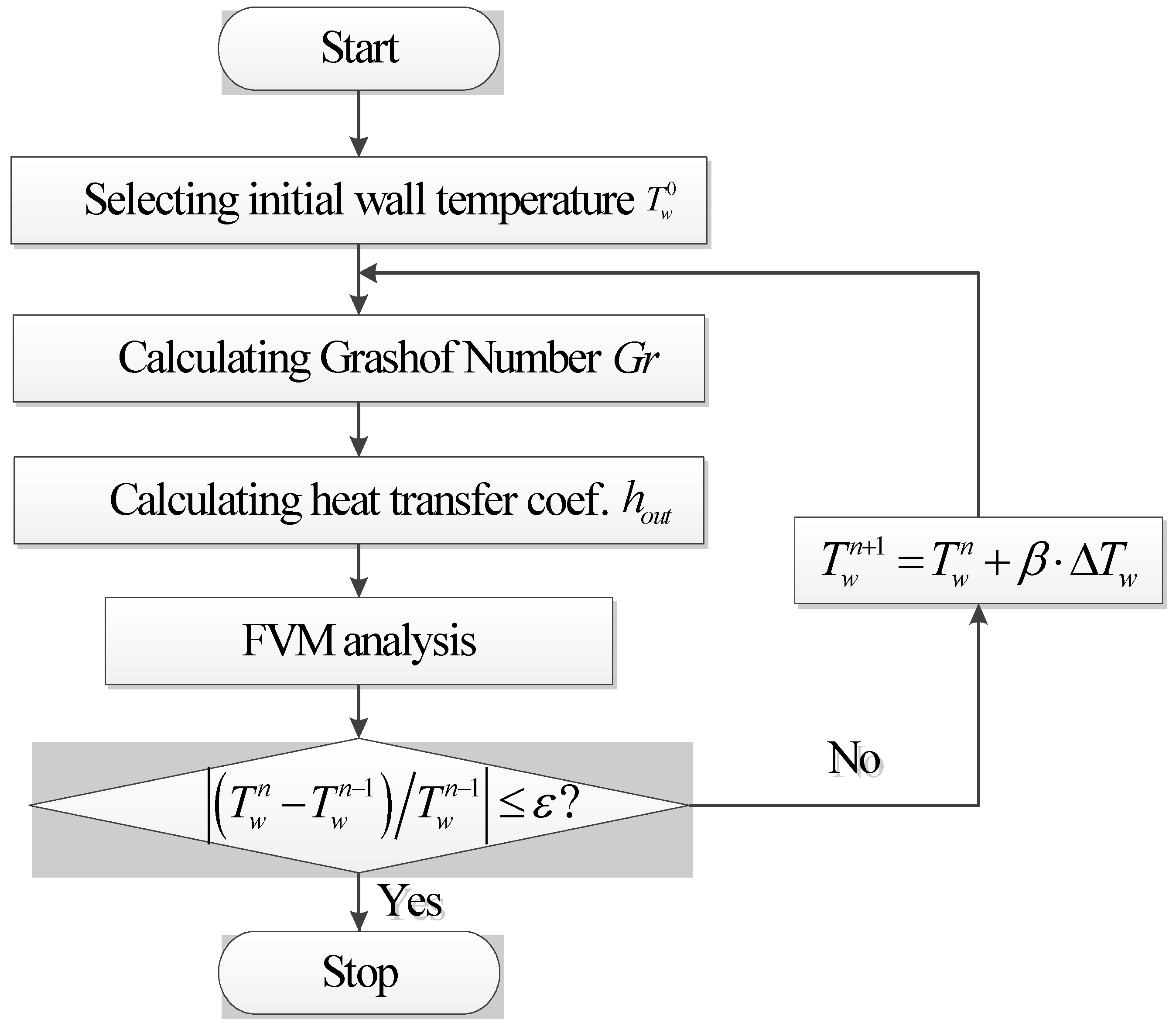
As can be seen in Equation (9), Grashof number Gr is adopted to estimate the convection heat transfer coefficient under the condition of free convection, however, wall temperature T_w cannot be determined before the temperature field of the TFPMLM is obtained. In order to obtain the accurate distribution of the TFPMLM temperature field, an estimated value of initial wall temperature $T_{\text{w}}^0$ and iterative calculation of the TFPMLM temperature field are necessary.

Table 3. Constants in Equation (9).

Geometries	Flow conditions	C	n	Gr
Vertical planes and cylinders	Laminar flow	0.59	1/4	1.43 × 104–3 × 109
	Transition	0.0292	0.39	3 × 109–2 × 1010
	Turbulent flow	0.11	1/3	>2 × 1010
Horizontal cylinders	Laminar flow	0.48	1/4	1.43 × 104–5.76 × 108
	Transition	0.0165	0.42	5.76 × 108–4.65 × 109
	Turbulent flow	0.11	1/3	>4.65 × 109

Table 3. Constants in Equation (9).

Geometries	Flow conditions	C	n	Gr
Vertical planes and cylinders	Laminar flow	0.59	1/4	1.43 × 104–3 × 109
	Transition	0.0292	0.39	3 × 109–2 × 1010
	Turbulent flow	0.11	1/3	>2 × 1010
Horizontal cylinders	Laminar flow	0.48	1/4	1.43 × 104–5.76 × 108
	Transition	0.0165	0.42	5.76 × 108–4.65 × 109
	Turbulent flow	0.11	1/3	>4.65 × 109

The flow diagram of iterative calculation is shown in Figure 8. A predicted wall temperature and corresponding convection heat transfer coefficient of casing outer surface are employed in the first-step calculation, thus gaining the first calculated value of wall temperature $T_{\text{w}}^1$. If the difference between $T_{\text{w}}^0$ and $T_{\text{w}}^1$ meets the permissible error ε, namely $\left|\left(T_{\text{w}}^n-T_{\text{w}}^{n-1}\right)/T_{\text{w}}^{n-1}\right|\le \text{ε}$, the calculation is completed. Otherwise a new wall temperature $T_{\text{w}}^{n+1}$ is selected according to Equation (10) and corresponding heat transfer coefficient is applied to the 3-D temperature field model as boundary condition. The permissible error ε is usually 0.5% and β is a coefficient within the range of 0 to 1:

$$\{\begin{array}{l}{T}_{\text{w}}^{n+1}=T_{\text{w}}^n+\text{β}\cdot \mathrm{\Delta }{T}_{\text{w}}\\ \mathrm{\Delta }{T}_{\text{w}}=T_{\text{w}}^n-T_{\text{w}}^{n-1}\end{array}$$

(10)

Figure 8. Flow diagram of the iterative calculation.

Figure 8. Flow diagram of the iterative calculation.

Obviously, the convection heat transfer coefficients associated with various air flow velocities are different in the forced convection system. When the air flow velocity u equals 1 m/s, convection heat transfer coefficients of each outer surface are indicated in Table 4.

Table 4. Convection heat transfer coefficients when u equals 1 m/s.

Surfaces	Convection heat transfer coefficients (W/m−2·K)	Surfaces	Convection heat transfer coefficients (W/m−2·K)
S1	0	S2	5.68
S3	6.98	S4	5.48
S5	30.8	S6	7.67
S7	12.7	S8	13.3
S9	6.34	S10	36.73

Table 4. Convection heat transfer coefficients when u equals 1 m/s.

Surfaces	Convection heat transfer coefficients (W/m−2·K)	Surfaces	Convection heat transfer coefficients (W/m−2·K)
S1	0	S2	5.68
S3	6.98	S4	5.48
S5	30.8	S6	7.67
S7	12.7	S8	13.3
S9	6.34	S10	36.73

3.2. Thermal Conductivity

The temperature field distribution of the TFPMLM is significantly dependent on the thermal conductivity of each component; the higher the thermal conductivity is, the more uniform the temperature field distribution is. There is an evident difference among thermal conductivities of materials employed in the TFPMLM. To be specific, the thermal conductivity of metallic material is approximately 10³ times that of insulation. In order to accurately compute the temperature variation rules of small sized regions or components with small thermal conductivity, multilayer meshes are adopted in such region. Meanwhile, reasonable simplifications are also needed.

The calculation of the thermal conductivities of stator core and equivalent insulation inside the stator slot are discussed in this section.

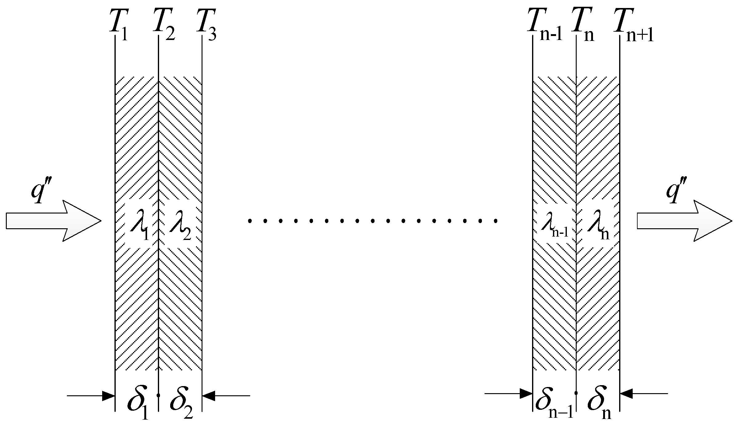
The surface of silicon-steel sheet is coated by insulating varnish with the thickness of approximate 0.01 mm to 0.02 mm, which decreases the thermal conductivity of stator core, and further affects the temperature field distribution of the TFPMLM. It is obviously difficult to model the stator core as the actual situation. Consequently, modeling stator lamination is simplified by considering it as a solid cylindrical region. In the radial and circumferential direction, the thermal conductivity of the solid region equals that of silicon steel. Conducting heat transfer along the axial direction of stator core is analogous to the process of conduction heat transfer throughout multi-layer plates which can be regarded as an alternative arrangement for insulating varnish and silicon steel [30]. The schematic diagram is shown in Figure 9, where λ_n, δ_n are thermal conductivity and thickness of each layer plate, respectively; T_n−1, T_n are temperatures of both sides of one plate; $q^{″}$ is heat flux density flowing through multi-layer plates.

Figure 9. Schematic diagram of the conduction heat transfer in multi-layer plates.

Figure 9. Schematic diagram of the conduction heat transfer in multi-layer plates.

Based on Fourier’s Law, $q^{″}$ can be determined as:

$$q^{″}=\frac{{\text{λ}}_1}{{\text{δ}}_1}(T_1-T_2)=\frac{{\text{λ}}_2}{{\text{δ}}_2}(T_2-T_3)=\cdots =\frac{{\text{λ}}_n}{{\text{δ}}_n}(T_n-T_{n+1})$$

(11)

The temperature difference between both ends of multi-layer plates can be deduced as:

$$T_{\text{1}}-T_{n\text{+1}}=q^{″}{\displaystyle \sum _{i=1}^n\frac{{\text{δ}}_i}{{\text{λ}}_i}}$$

(12)

The multi-layer plates are assumed as a solid component with effective thermal conductivity λ_eq:

$$q^{″}={\text{λ}}_{\text{eq}}(T_1-T_{n\text{+1}})/{\displaystyle \sum _{i=1}^n{\text{δ}}_i}$$

(13)

The effective thermal conductivity of multi-layer plates can be finally expressed as:

$${\text{λ}}_{\text{eq}}={\displaystyle \sum _{i=1}^n{\text{δ}}_i}/{\displaystyle \sum _{i=1}^n\frac{{\text{δ}}_i}{{\text{λ}}_i}}$$

(14)

For the lamination of the machine, it is assumed that the equivalent thicknesses of silicon-steel sheet and insulating varnish are δ_Fe, δ₀, respectively, and the thermal conductivities of them are λ_Fe, λ₀, respectively. The equivalent thermal conductivity of lamination along the axial direction can be calculated as:

$${\text{λ}}_{\text{Fez}}=\frac{{\text{δ}}_{\text{Fe}}+{\text{δ}}_0}{\frac{{\text{δ}}_{\text{Fe}}}{{\text{λ}}_{\text{Fe}}}+\frac{{\text{δ}}_0}{{\text{λ}}_0}}$$

(15)

For the TFPMLM prototype, the stator windings are composed of copper wires which are randomly distributed in the slot, and the gap among copper wires are filled with air. Because of the small size of insulating varnish and gap, an equivalent model is used to simulate the actual heat conduction in the stator slot. The equivalent model consists of three parts: solid copper conductor, equivalent insulation and slot insulation [31]. The solid copper conductor is located in the middle of the slot, and its area equals that of total copper wires in one slot. The slot insulation surrounds the inner wall of the slot. The equivalent insulation which is a combination of insulating varnish and gap occupies the rest of the space in the slot, as illustrated in Figure 10. The effective thermal conductivity of the equivalent insulation can be calculated as:

$${\text{λ}}_{\text{in}}\text{=}\frac{{\text{δ}}_{\text{v}}+{\text{δ}}_{\text{g}}}{\frac{{\text{δ}}_{\text{v}}}{{\text{λ}}_{\text{v}}}+\frac{{\text{δ}}_{\text{g}}}{{\text{λ}}_{\text{g}}}}$$

(16)

where δ_v, δ_g are equivalent thicknesses of varnish and gap, respectively; λ_v, λ_g are thermal conductivities of varnish and gap, respectively.

Therefore, the complicated composition in the stator slot is simplified to three components composed of thermally isotropic materials.

Figure 10. Simplification for the components in the stator slot.

Figure 10. Simplification for the components in the stator slot.

The thermal conductivities of the materials involved in the TFPMLM are listed in Table 5.

Table 5. Thermal conductivities of different components.

Components	Thermal conductivity (W/m·K)	Components	Thermal conductivity (W/m·K)
Casing	202	Slot	0.22
Stator core	46/46/3.6	Equivalent insulation	0.048
Stator winding	398	Mover yoke	46/46/3.6
PM	9	Non-magnetic ring	0.2

Table 5. Thermal conductivities of different components.

Components	Thermal conductivity (W/m·K)	Components	Thermal conductivity (W/m·K)
Casing	202	Slot	0.22
Stator core	46/46/3.6	Equivalent insulation	0.048
Stator winding	398	Mover yoke	46/46/3.6
PM	9	Non-magnetic ring	0.2

3.3. Losses

The losses generated during the electromechanical energy conversion directly result in the heating of the machine. The losses in the TFPMLM include Ohmic loss, stator core loss, eddy current losses of the PMs and mover yoke, and mechanical loss. The 3-D transient electromagnetic field analysis in our foregoing research is employed to determine the losses in the machine [15].

Based on the widely accepted Bertotti’s iron-loss model, the core loss in the stator lamination consists of hysteresis loss, classical eddy current loss and excess loss, respectively [32]:

$$P_{\text{Fe}}=K_{\text{h}}f{B}_{\text{m}}^2+K_{\text{c}}{(f{B}_{\text{m}})}^2+K_{\text{e}}{(f{B}_{\text{m}})}^{1.5}$$

(17)

where P_Fe is core loss; K_h is hysteresis core loss coefficient; K_c is eddy current core loss coefficient; K_e is excess core loss coefficient; B_m is amplitude of flux density; f is frequency.

The average value of the eddy current loss in the PMs or mover yoke during one machine cycle is computed by:

$$P_{\text{e}}=\frac{1}{T}{\displaystyle {\int }_T{\displaystyle \sum _{i=1}^k{J}_{\text{e}}^2{\mathrm{\Delta }}_{\text{e}}}}{\text{σ}}^{-1}\text{d}t$$

(18)

where P_e is eddy current loss; J_e is eddy current density in element; Δ_e is element volume; σ is conductivity; T is cycle of time.

The Ohmic loss is computed by $I^{2}R$. The losses listed in Table 6 are calculated for the prototype under the rated operating condition (I_N = 8 A) and applied to the temperature field model as heat sources in the thermal analysis. The Ohmic loss accounts for the greatest proportion of the total loss. The eddy current loss in the PMs is much more than that in the mover core.

Table 6. Losses in the TFPMLM.

Components	Loss (W)	Components	Loss (W)
Winding	62.37	Stator core	4.36
PMs	0.864	Mover core	0.246

Table 6. Losses in the TFPMLM.

Components	Loss (W)	Components	Loss (W)
Winding	62.37	Stator core	4.36
PMs	0.864	Mover core	0.246

4. Results and Analysis

Based on the 3-D temperature field model of the TFPMLM, the commercial software Fluent solver was used to solve the heat conduction differential equation with the corresponding boundary conditions, and the temperature field distribution and variation rule are obtained.

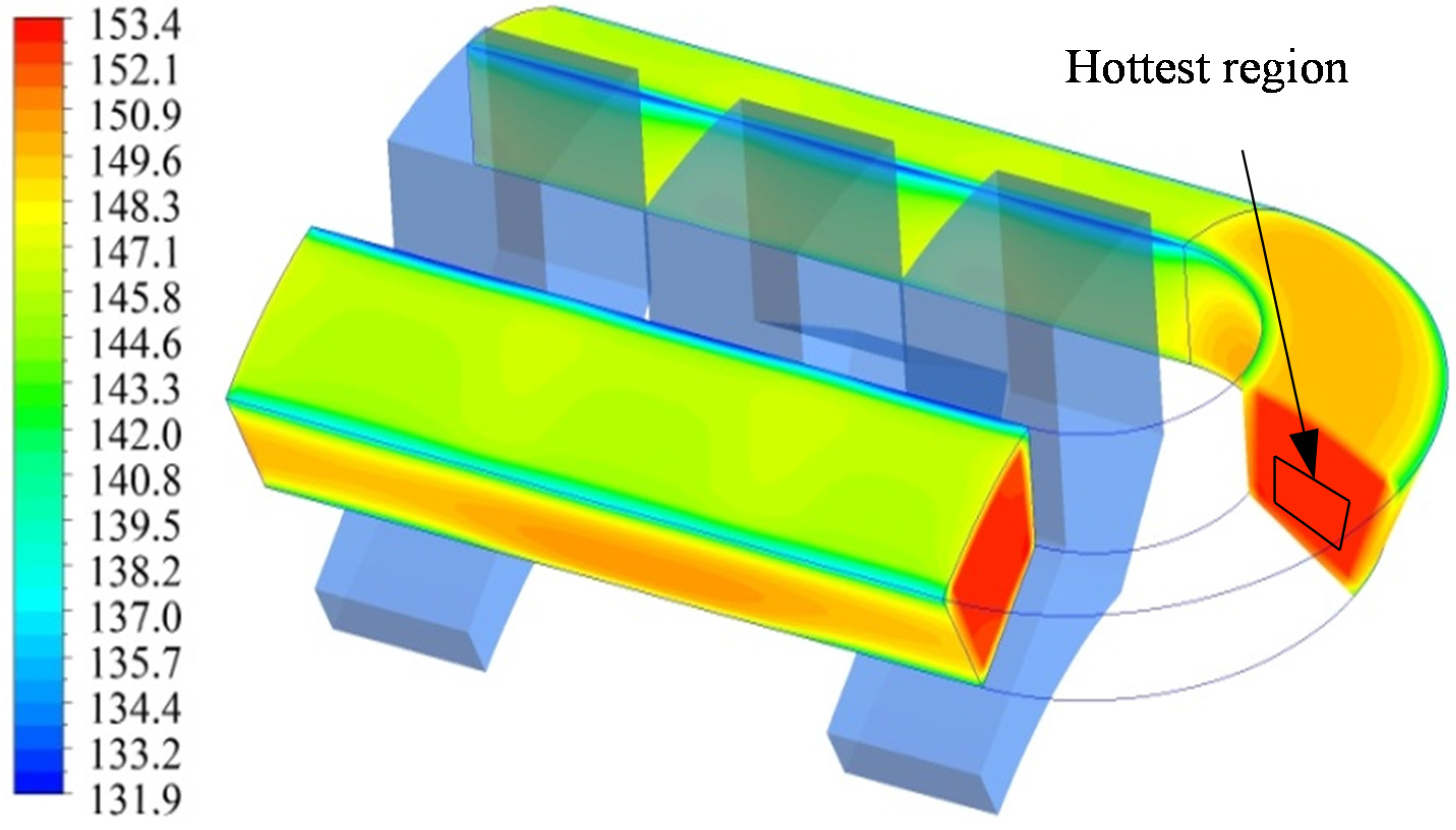
Figure 11 shows the temperature field distribution of the stator winding, where the blue transparent parts refer to the stator teeth. The winding temperature decreases gradually from the inside to the outside. In the axial direction, the winding temperature decreases a little from the end winding to the axially central position. The temperature at the middle cross section of the end winding is the highest with the temperature of 153.4 °C, as illustrated in Figure 11. Due to the limited air flow velocity, the heat transfer coefficient is low. Consequently, the cooling effect of convection heat transfer is poorer than that of conduction heat transfer. Since the end winding can only transfer the heat to the equivalent insulation which is cooled by way of convection heat transfer with the air in the casing, the temperature of the end winding is higher than that of the straight part of the winding which can transfer the heat to the equivalent insulation, slot insulation, stator core and casing.

Figure 11. Temperature field distribution of the stator winding (in °C).

Figure 11. Temperature field distribution of the stator winding (in °C).

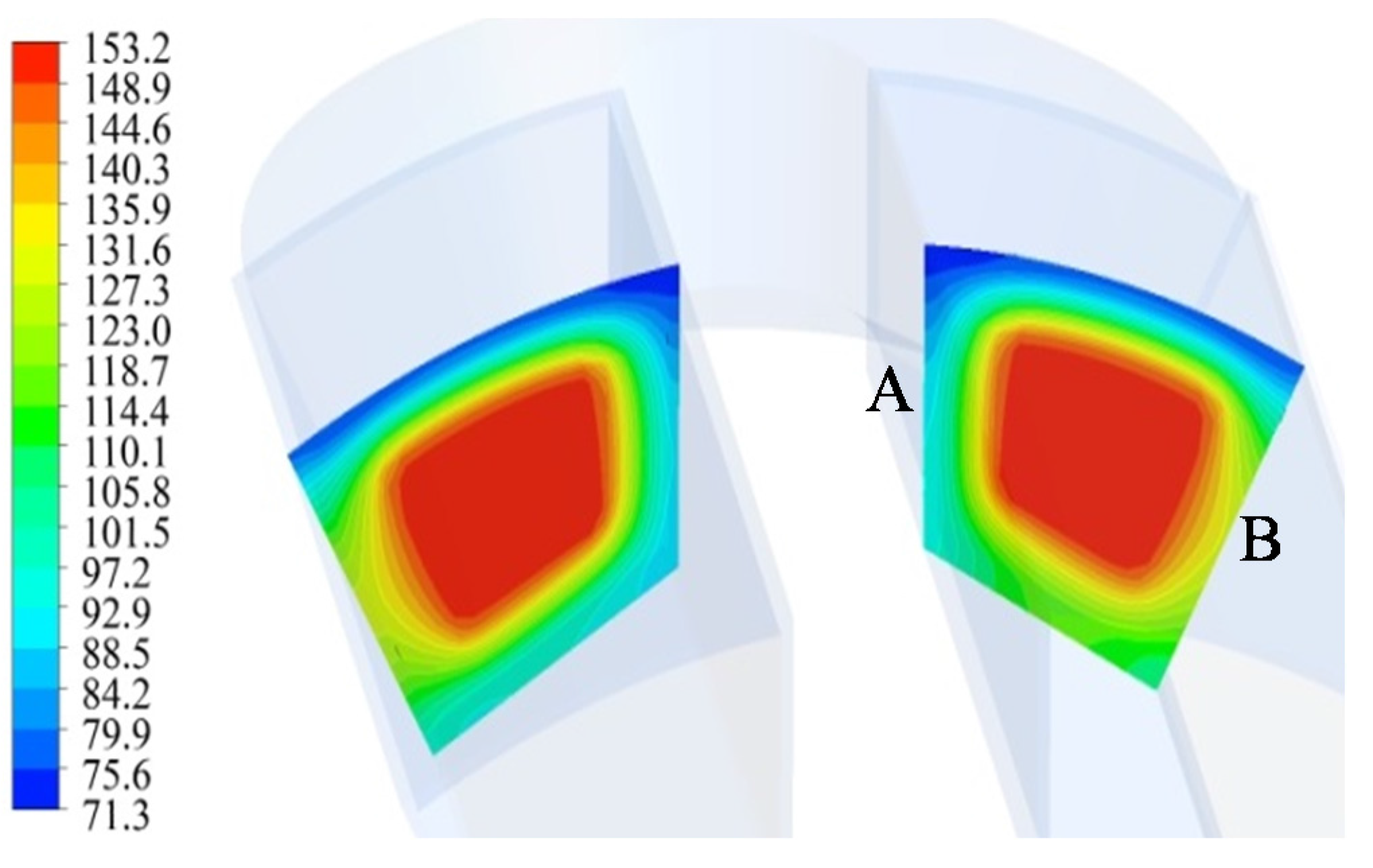
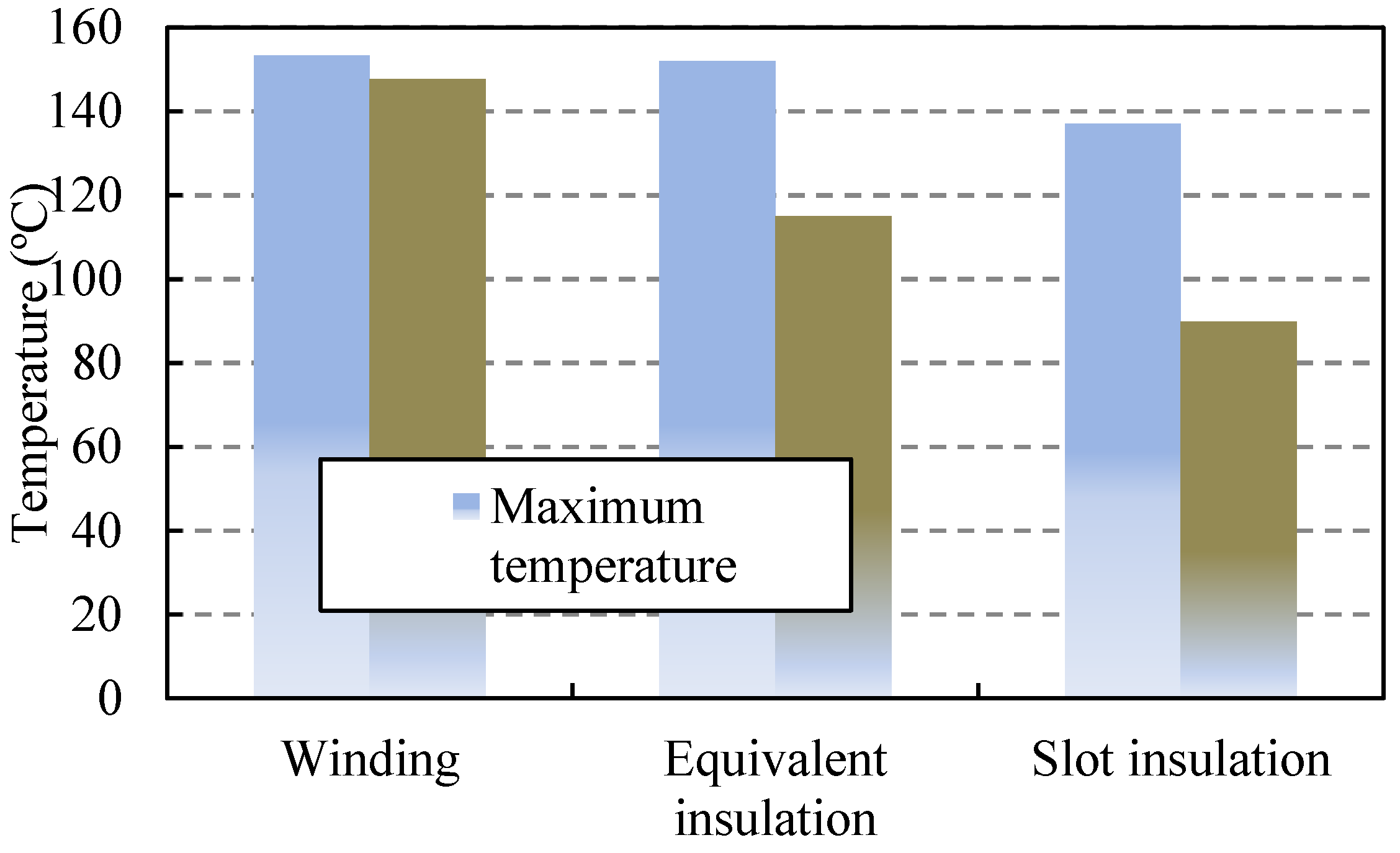
Figure 12 shows the temperature variation in the stator slot at one sixth of the axial direction. Since copper has high thermal conductivity, the internal temperature of the winding tends to be consistent. The average temperature of the winding is 147.7 °C which is 5.7 °C lower than the maximum temperature. Since the thermal conductivity of the slot insulation and equivalent insulation are lower, the temperature gradient variation at the positions of the equivalent insulation and slot insulation is quite obvious. The maximum and the average temperatures of the stator winding, equivalent insulation and slot insulation are shown in Figure 13. The temperature of Side A, the contact side between the winding and stator tooth, is slightly lower than that of Side B, the contact side between two adjacent windings.

Figure 12. Temperature field distribution at an axial cross section (in °C).

Figure 12. Temperature field distribution at an axial cross section (in °C).

Figure 13. Maximum and average temperatures in the slot.

Figure 13. Maximum and average temperatures in the slot.

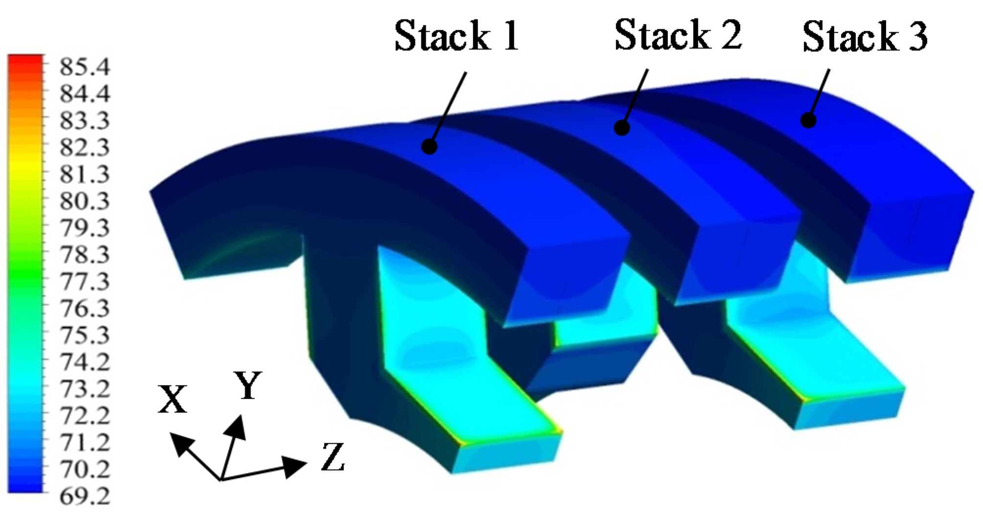
Figure 14 shows the temperature field distribution of the stator core. The temperature of the stator tooth and stator yoke which are in direct contact with the winding is higher than that of the stator yoke back; the maximum temperature of the overall stator tooth is 11.2 °C higher than that of the stator yoke. Three stacks of laminations are numbered as 1 to 3 as illustrated in Figure 14. Stack 1 is close to the axial center, and Stack 3 is close to the end winding. The core loss of Stack 3 is larger than that of Stack 1, however, the average temperature of Stack 3 is 0.52 °C lower than that of Stack 1. This is because Stack 3 which is exposed to the fluid air in the casing can not only conduct heat to the casing, but also be cooled by the fluid air in the casing. Therefore, the heat-dissipating condition of Stack 3 is much better than that of Stack 1.

Figure 14. Temperature field distribution of the stator core (in °C).

Figure 14. Temperature field distribution of the stator core (in °C).

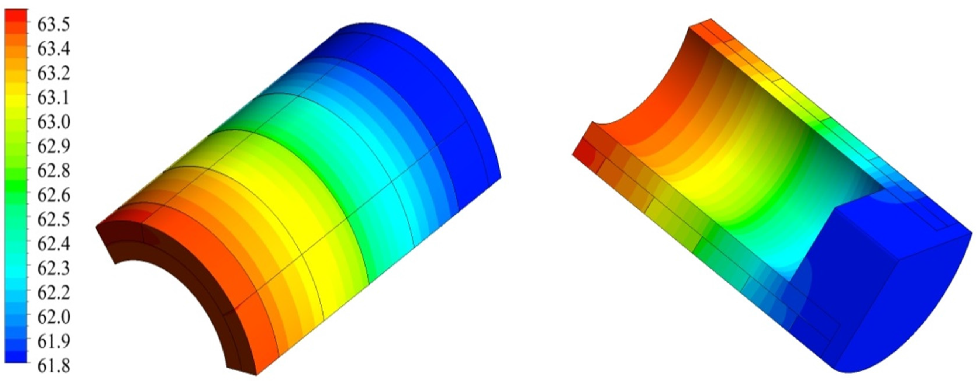
The temperature field distribution of the PMs and mover yoke is shown in Figure 15. The temperature of the PMs is distributed homogeneously in the circumferential direction, but gradually decreases from the axial center to the end along the axial direction, which is not affected by the adhesive coatings among PMs and different densities of the eddy current loss in the PMs. Since the eddy current loss in the PMs is small, the temperature of the PMs is within the range of 61.8–63.5 °C. The temperature field distribution of the mover yoke is consistent with that of the PMs, and the maximum temperature of the mover yoke is 63.5 °C. Since the heat transfer coefficient of Surface S10 is much higher than that of Surface S9, most of the heat generated in the PMs is firstly transferred to the mover yoke by the way of conduction heat transfer and then to the air from the outer surface of the mover, resulting in an obvious tendency that the temperature decreases gradually from the axial center to the end.

Figure 15. Temperature field distribution of the PMs and mover yoke (in °C).

Figure 15. Temperature field distribution of the PMs and mover yoke (in °C).

5. Influence of Slot Filling Factor on the Temperature Field

The slot filling factor is an important parameter of the electrical machine design. The higher slot filling factor can improve the compactness of the machine, but will increase the difficulty and processing hours for inserting windings. What is more, the slot filling factor has a significant impact on the heat dissipation capability of the windings which are normally the hottest parts in the machine. In the analyzed machine whose slot filling factor is 61%, the thermal conductivity of the equivalent insulation is 0.048 W/(m·K) which is much smaller than that of the varnish. Due to the existence of the gap in the stator slot, the thermal conductivity of the equivalent insulation is greatly reduced, thus affecting the heat dissipation of the stator windings. In this section, a detailed calculation and analysis of the impact of the slot filling factor on the temperature rise are carried out.

The 3-D temperature field model of the TFPMLM is re-established with the slot filling factor of 66%, 71% and 76%, respectively. With the slot filling factor increased, the equivalent thickness of the varnish increases, while the equivalent thickness of the gap decreases. The corresponding thermal conductivities of the equivalent insulation in the slot are listed in Table 7.

The increasing of the slot filling factor can be realized by the way of increasing wire diameter. In the first, the losses in the analyzed machine are kept constant in order to investigate the independent effect of increasing the slot filling factor (Case A).

Table 7. The effective thermal conductivities of the TFPMLM with different slot filling factors.

Slot filling factor	Equivalent thickness (mm)		Effective thermal conductivity (W/m·K)
	Varnish	Gap
61%	0.827	1.061	0.048
66%	0.860	0.927	0.052
71%	0.892	0.781	0.057
76%	0.921	0.638	0.063

Table 7. The effective thermal conductivities of the TFPMLM with different slot filling factors.

Slot filling factor	Equivalent thickness (mm)		Effective thermal conductivity (W/m·K)
	Varnish	Gap
61%	0.827	1.061	0.048
66%	0.860	0.927	0.052
71%	0.892	0.781	0.057
76%	0.921	0.638	0.063

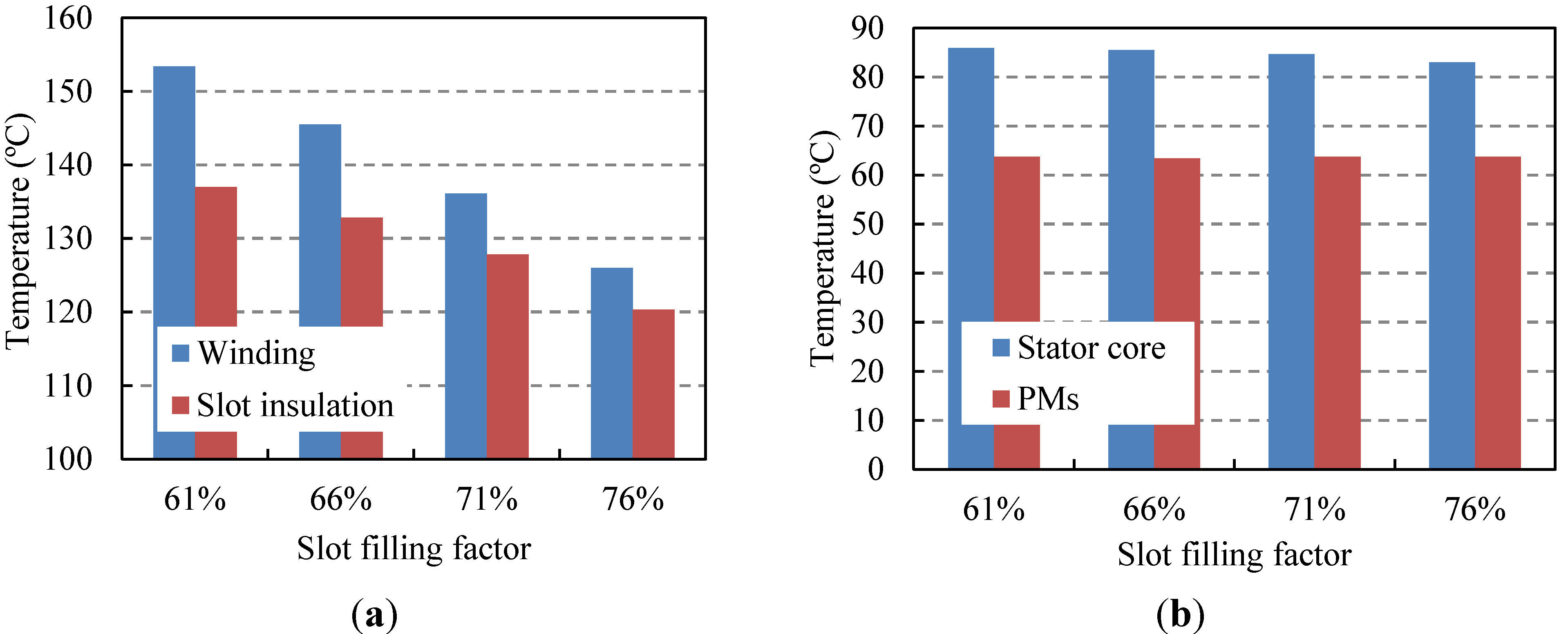
After the thermal calculation of the machine with different slot filling factors, the maximum temperatures of the stator winding and the slot insulation are shown in Figure 16a. When the slot filling factor is increased, the maximum temperatures of both the stator winding and slot insulation decrease gradually. The reason is when the slot filling factor is increased continuously, the high thermal conductivity materials such as copper will occupy a greater and greater proportion of the space in the slot, the effective thermal conductivity of the equivalent insulation in the slot will increase accordingly, and the heat generated by the stator winding will be transferred from the slot inside to the slot outside more effectively. When the slot filling factor is 61%, 66%, 71% and 76%, the maximum temperature of the stator winding is 153.4 °C, 145.5 °C, 136.1 °C and 126.0 °C, respectively. The difference between two adjacent temperatures is 7.9 °C, 9.4 °C and 10.1 °C, which shows the higher the slot filling factor is, the more obvious the improvement in cooling effect is. The maximum temperatures of the stator core and PMs are shown in Figure 16b. It can be seen that the maximum temperature of the stator core decreases a little and the temperature of the PMs is not affected by the improvement of the heat dissipation condition in the stator slot.

Figure 16. The maximum temperatures of different parts vs. slot filling factor (Case A): (a) winding and slot insulation; (b) stator core and PMs.

Figure 16. The maximum temperatures of different parts vs. slot filling factor (Case A): (a) winding and slot insulation; (b) stator core and PMs.

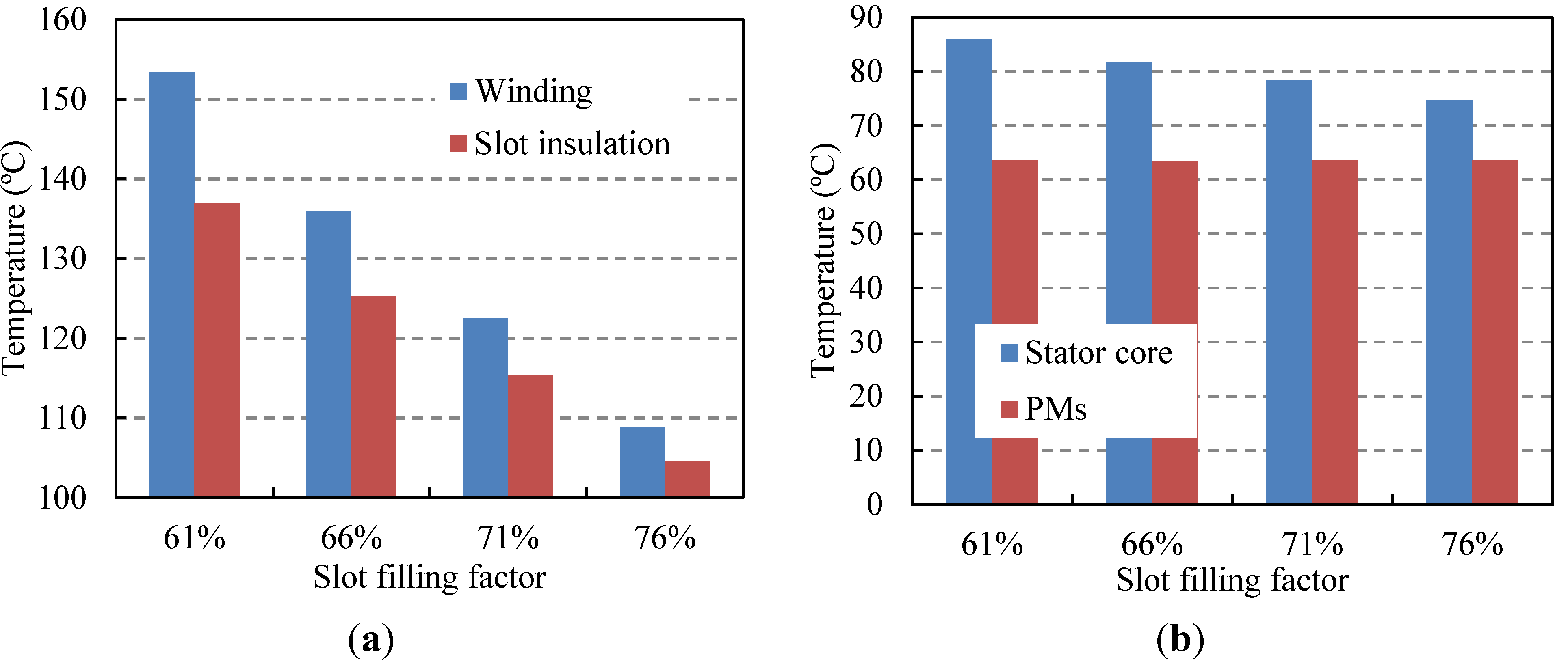
Actually, with the slot filling factor increased by way of increasing the wire diameter, the Ohmic loss is reduced. With the reduction of the Ohmic loss taken into account, the resultant effect of increasing slot filling factor is researched (Case B). The maximum temperatures of the different parts in the machine are shown in Figure 17. Compared with Case A, the temperatures of the stator winding and the slot insulation decrease more significantly. When the slot filling factor is increased from 61% to 76%, the temperatures of the stator winding and the slot insulation decrease 44.5 °C and 32.5 °C, which are larger than those in Case A (17.1 °C and 15.8 °C), respectively. 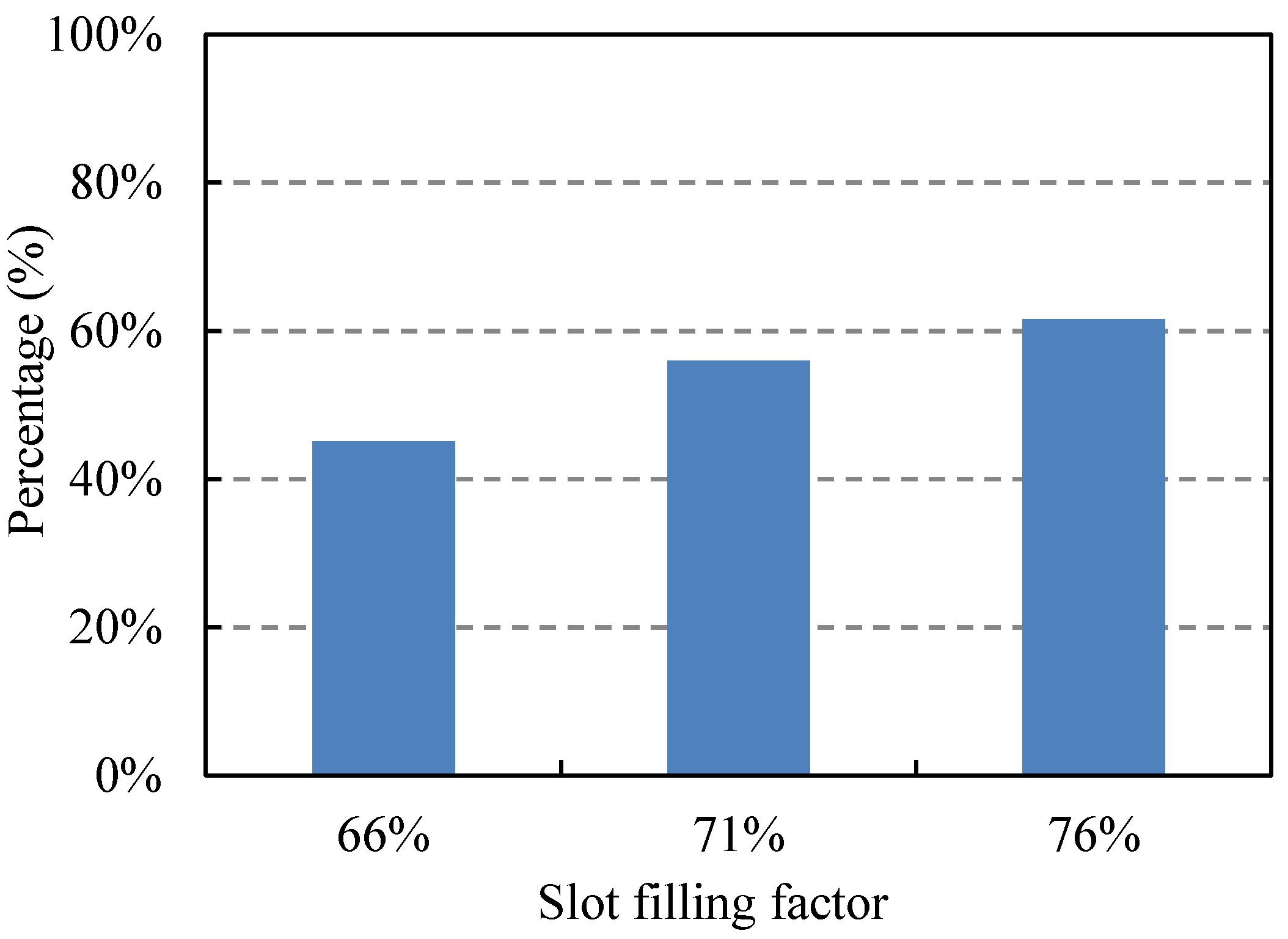Figure 18 shows the proportion of the winding temperature drops independently caused by increasing the wire diameter in the total temperature drop, which becomes larger and larger as the slot filling factor increases.

Figure 17. The maximum temperatures of different parts vs. slot filling factor (Case B): (a) winding and slot insulation; (b) stator core and PMs.

Figure 17. The maximum temperatures of different parts vs. slot filling factor (Case B): (a) winding and slot insulation; (b) stator core and PMs.

Figure 18. The proportion of winding temperature drop independently caused by increasing the wire diameter.

Figure 18. The proportion of winding temperature drop independently caused by increasing the wire diameter.

6. Influence of Loss Variation on the Temperature Field

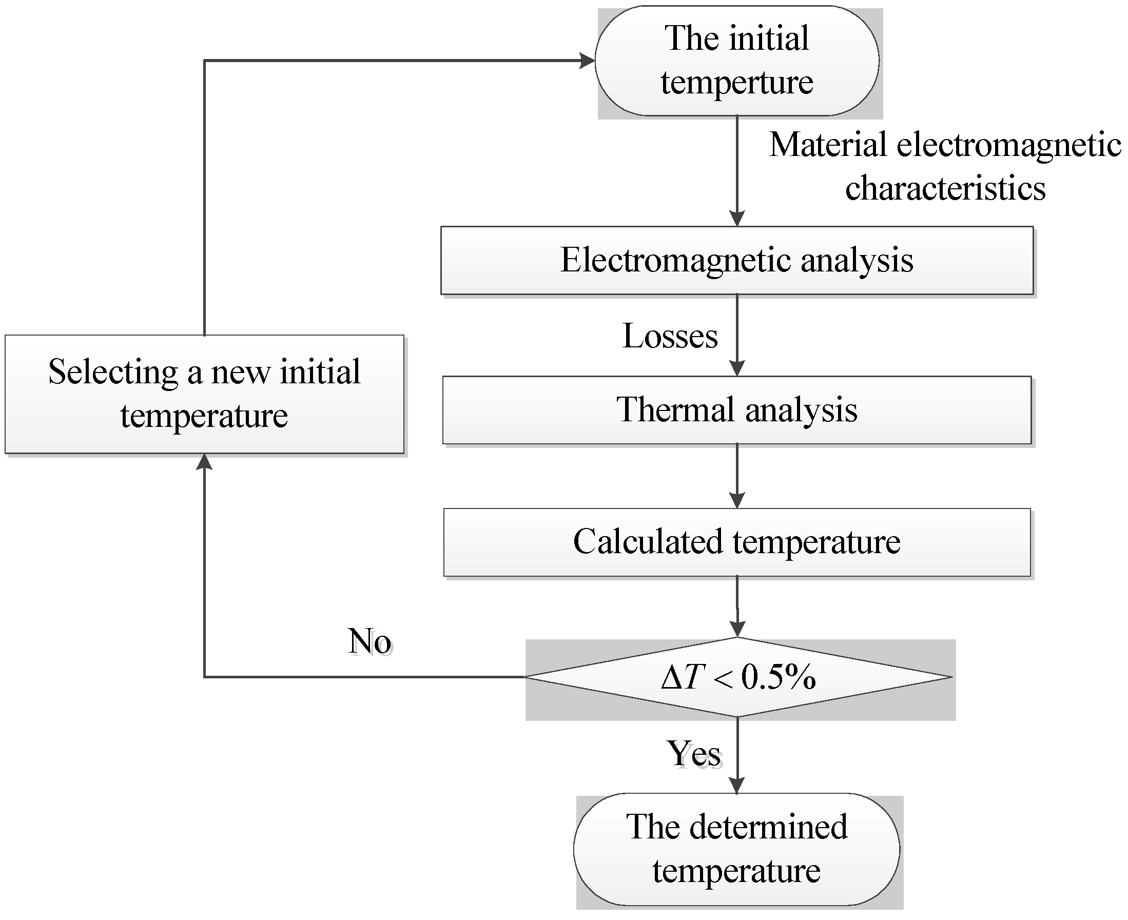
The losses of different parts in the machine exactly change with the temperature rise. The material electromagnetic characteristics are sensitive to temperature, especially the resistance and residual flux density. An iterative process combining electromagnetic and thermal analysis is performed to investigate the influence of loss variation on the temperature field. Figure 19 shows the flow diagram of iterative process. Initial temperatures T_ini of different parts are firstly selected, and corresponding material electromagnetic characteristics are adopted in the electromagnetic analysis. Thus losses of different parts are obtained and applied to the thermal analysis as heat sources. A new temperature field distribution is determined, then the initial temperatures are replaced with the calculated ones T_cal obtained from the thermal analysis. The next step of iterative calculation will be done, until the relative temperature error ΔT between T_ini and T_cal is less than the permissible error (0.5%).

Figure 19. Flow diagram of electromagnetic and thermal iteration.

Figure 19. Flow diagram of electromagnetic and thermal iteration.

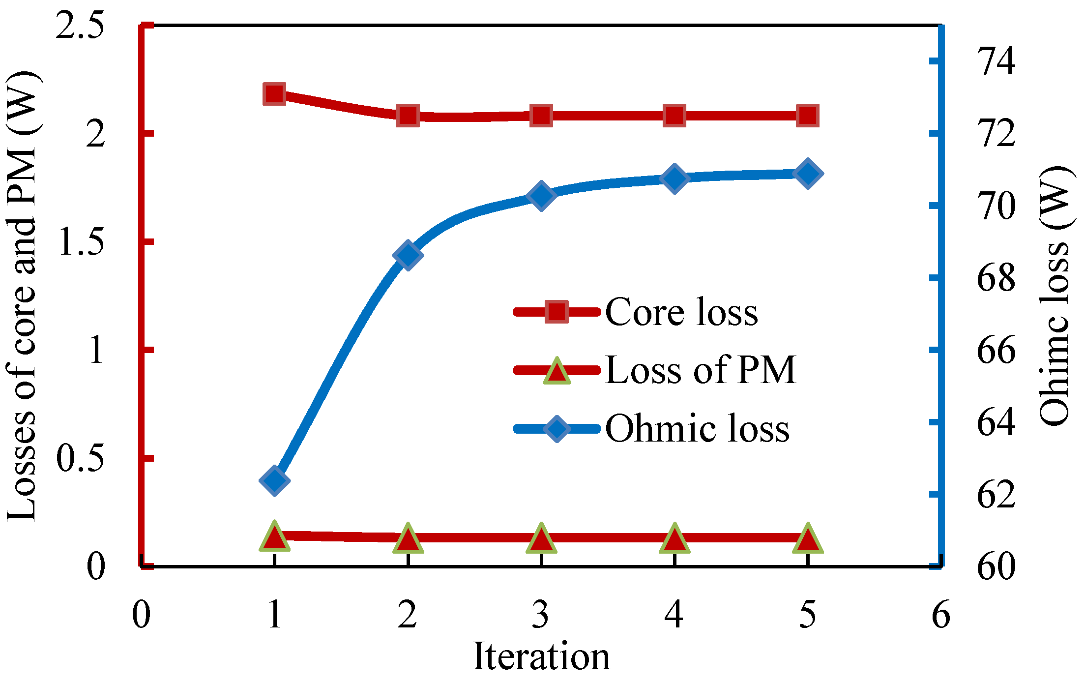
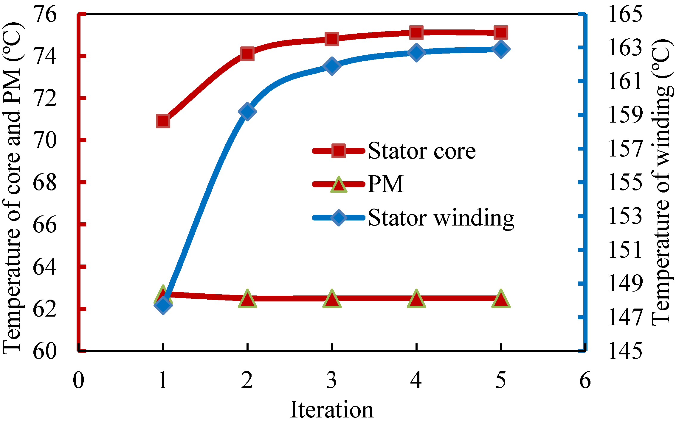
Figure 20 and Figure 21 show the variations of the losses and maximum temperatures versus the iteration step, respectively. Due to the temperature rise of PM, the residual flux density decreases, leading to both the losses of PM and stator core decrease. In every iterative step, the calculated temperature of winding is higher than the initial one, making the next initial temperature assumed higher than the last initial one. Consequently, the resistance of winding, of course, as well as the Ohmic loss increases gradually in the iterative process. Although the core loss decreases slightly, the temperature of core increases due to the temperature increase of winding. After five times iterations, all relative temperature errors of the stator winding, core, and PM meet the requirement. The final temperature of stator winding with the value of 162.9 °C is 15.2 °C higher than the initial one. The final temperature of PM decreases 0.2 °C, and that of core increase 4.2 °C.

Figure 20. Losses vs. iteration.

Figure 20. Losses vs. iteration.

Figure 21. Average temperature vs. iteration.

Figure 21. Average temperature vs. iteration.

7. Influence of Air Flow Velocity on the Temperature Field

As the TFPMLM reciprocates at different frequencies, the cooling air in the casing is forced to move at various speeds. Cooling air speed plays an important role in determining the heat transfer coefficients of the surfaces under forced convection heat transfer, thus affecting the temperature field distribution of the TFPMLM. The relation between air flow velocity and temperature field of the TFPMLM is analyzed in this section.

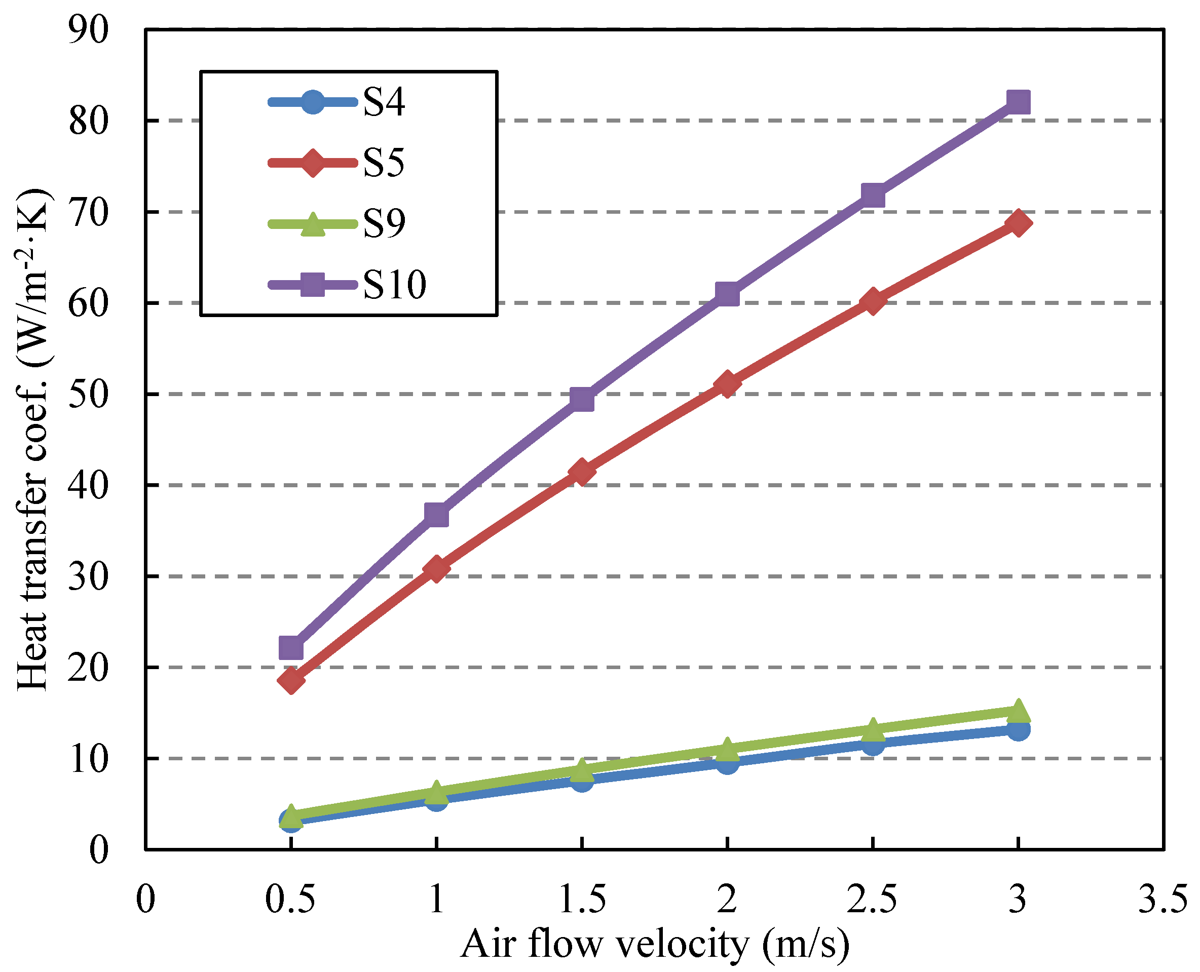
The heat transfer coefficients of the surfaces S4, S5, S9 and S10 are computed according to Section 3 while air flow velocity varies from 0.5 m/s to 3 m/s. As shown in Figure 22, the heat transfer coefficients of the vertical surfaces S5, S10 are far higher than those of the horizontal surfaces S4, S9. Meanwhile, with flow velocity increasing, the increments of the heat transfer coefficients of S5, S10 are also much higher than those of S4, S9. When air flow velocity is 3 m/s, the heat transfer coefficients of the surfaces S5, S10 are at a high range of 70–80 W/m⁻²·K.

Figure 22. The convection heat transfer coefficients vs. air flow velocity.

Figure 22. The convection heat transfer coefficients vs. air flow velocity.

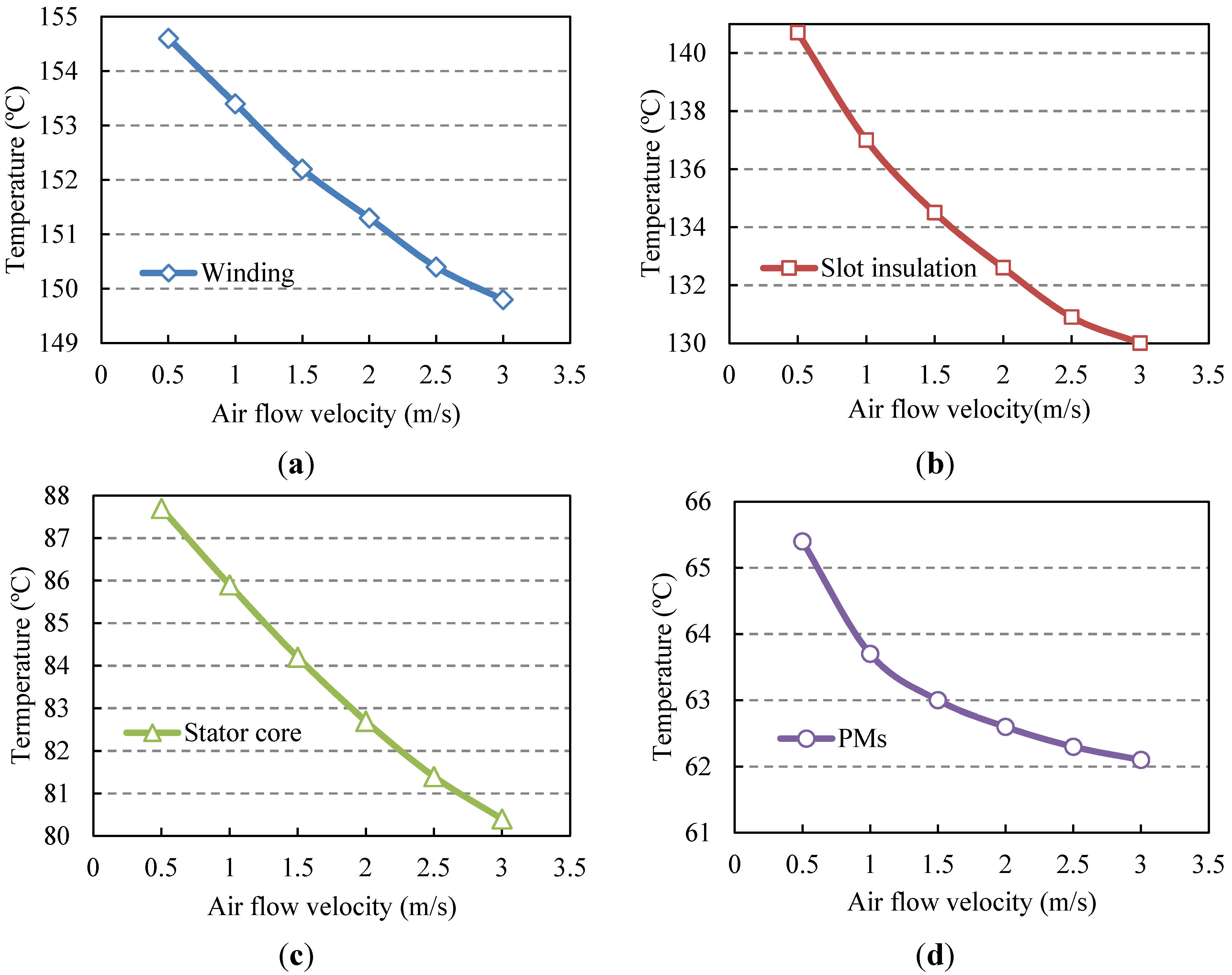
Figure 23 shows the variations of the maximum temperature versus air flow velocity. Due to the increment of the air flow velocity, the cooling effect of the TFPMLM is strengthened, and therefore the temperature rise of each part in the TFPMLM declines. When air flow velocity increases from 0.5 m/s to 3 m/s, the temperature of the stator winding rises, and slot insulation, stator core and PMs decline 4.8 °C, 10.7 °C, 7.3 °C and 3.3 °C, respectively, while the decreasing ratios are 3.1%, 7.6%, 8.3%, 5.0%, respectively. The cooling effect improvement of the parts which contact the air directly, namely slot insulation and stator core, is more significant than that of other parts. The eddy current loss in the PMs is very small and consequent temperature rise is low; hence, the cooling effect improvement of the PMs is unremarkable.

It is noteworthy that the largest temperature decline in the PMs occurs within the air speed range of 0.5 m/s to 1 m/s. The temperature rise in the PMs decreases 1.7 °C, 0.7 °C, 0.4 °C, 0.3 °C, 0.2 °C, respectively, when air flow velocity increases from 0.5 m/s to 3 m/s, as shown in Figure 23d. Owing to the transition from laminar to turbulent flow of the cooling air, the convection heat transfer capacity boosts conspicuously within the range of 0.5 m/s to 1 m/s. When cooling air is in the state of fully developed turbulence, the increasing extent of the heat transfer capacity is attenuate.

Figure 23. The maximum temperatures of different parts vs. air flow velocity: (a) winding; (b) slot insulation; (c) stator core; and (d) PMs.

Figure 23. The maximum temperatures of different parts vs. air flow velocity: (a) winding; (b) slot insulation; (c) stator core; and (d) PMs.

8. Conclusions

(1) The hottest spot of the TFPMLM appears in the middle of the end winding. Since the cooling effect of convection heat transfer is poorer than that of conduction heat transfer in the analyzed machine, the temperature of the end winding is a little higher than that of the straight part of the stator winding. The regional temperature of the stator core adjoining the stator winding is higher than that of the stator yoke back. Due to the small eddy current loss of the PMs with the temperature rise of 3.7 K, there is no risk of demagnetization caused by excessive temperature rise.

(2) The increase of the slot filling factor considerably improves the heat dissipation capability of the stator winding. As the effective thermal conductivity increases with the slot filling factor increased, more heat is transferred from the slot inside to the slot outside, causing the temperatures of the stator winding and the slot insulation to decrease.

(3) The increasing of the air flow velocity boosts the convection heat transfer in the TFPMLM. When the air flow velocity increases from 0.5 m/s to 3 m/s, the temperature of the stator winding decreases 4.8 °C. With the increase in air flow velocity, the temperature of the part which is exposed to the cooling air such as stator core decreases the most. Moreover, this advantageous effort is the most prominent when the cooling air is in transition from laminar flow to developed turbulent flow.

References

- Abd-Rabou, A.S.; Hasanien, H.M.; Sakr, S.M. Design development of permanent magnet excitation transverse flux linear motor with inner mover type. IET Electr. Power Appl. 2010, 4, 559–568. [Google Scholar] [CrossRef]
- Polinder, H.; Mecrow, B.C.; Jack, A.G.; Dickinson, P.G.; Mueller, M.A. Conventional and TFPM linear generators for direct-drive wave energy conversion. IEEE Trans. Energy Convers. 2005, 20, 260–267. [Google Scholar] [CrossRef]
- Bang, D.; Hwang, S.H.; Kim, J.W.; Hwang, W.; Han, P.W. Bearingless transverse flux permanent magnet machine for large direct-drive. In Proceedings of the IEEE Energy Conversion Congress and Exposition (ECCE 2014), Pittsburg, PA, USA, 14–18 September 2014; pp. 4874–4880.
- Vining, J.; Lipo, T.A.; Venkataramanan, G. Design and optimization of a novel hybrid transverse/longitudinal flux, wound-field linear machine for ocean wave energy conversion. In Proceedings of the IEEE Energy Conversion Congress and Exposition (ECCE 2009), Helsinki, Finland, 20–24 September 2009; pp. 3726–3733.
- Zheng, P.; Tong, C.D.; Chen, G.; Liu, R.R.; Sui, Y.; Shi, W. Research on the Magnetic Characteristic of a Novel Transverse-Flux PM Linear Machine Used for Free-Piston Energy Converter. IEEE Trans. Energy Convers. 2011, 47, 1082–1085. [Google Scholar] [CrossRef]
- Kang, D.H.; Weh, H. Design of an integrated propulsion, guidance, and levitation system by magnetically excited transverse flux linear motor (TFM-LM). IEEE Trans. Energy Convers. 2004, 19, 477–484. [Google Scholar] [CrossRef]
- Hwang, S.H.; Kim, J.M.; Bang, D.J.; Kim, J.W.; Koo, D.H.; Kang, D.H. Control of independent multi-phase transverse flux linear synchronous motor based on magnetic levitation. In Proceedings of the Applied Power Electronics Conference and Exposition (APEC 2014), Fort Worth, TX, USA, 16–20 March 2014; pp. 2488–2491.
- Zhao, M.; Zou, J.M.; Xu, Y.X.; Zou, J.B.; Wang, Q. The Thrust Characteristic Investigation of Transverse Flux Tubular Linear Machine for Electromagnetic Launcher. IEEE Trans. Plasma Sci. 2011, 39, 925–930. [Google Scholar] [CrossRef]
- Fair, H.D. Advances in Electromagnetic Launch Science and Technology and Its Applications. IEEE Trans. Magn. 2009, 45, 225–230. [Google Scholar] [CrossRef]
- Hasanien, H.M. Particle Swarm Design Optimization of Transverse Flux Linear Motor for Weight Reduction and Improvement of Thrust Force. IEEE Trans Ind. Electr. 2011, 58, 4048–4056. [Google Scholar] [CrossRef]
- Chang, J.; Kang, D.; Lee, J.; Hong, J. Development of transverse flux linear motor with permanent-magnet excitation for direct drive applications. IEEE Trans. Magn. 2005, 41, 1936–1939. [Google Scholar] [CrossRef]
- Hong, D.K.; Woo, B.C.; Koo, D.H.; Kang, D.H. Optimum Design of Transverse Flux Linear Motor for Weight Reduction and Improvement Thrust Force Using Response Surface Methodology. IEEE Trans. Magn. 2008, 44, 4317–4320. [Google Scholar] [CrossRef]
- Hasanien, H.M.; Abd-Rabou, A.S.; Sakr, S.M. Design Optimization of Transverse Flux Linear Motor for Weight Reduction and Performance Improvement Using Response Surface Methodology and Genetic Algorithms. IEEE Trans. Energy Convers. 2010, 25, 598–605. [Google Scholar] [CrossRef]
- Yan, H.Y.; Yu, B.; Chong, X.; Song, Z.Y.; Lin, J.; Zheng, P. Research on a novel tubular transverse-flux permanent-magnet linear machine for free-piston energy converter. In Proceedings of the Electrical Machines and Systems (ICEMS 2011), Beijing, China, 20–23 August 2011; pp. 1–5.
- Zheng, P.; Yu, B.; Yan, H.Y.; Sui, Y.; Bai, J.G.; Wang, P.W. Electromagnetic analysis of a novel cylindrical transverse-flux permanent-magnet linear machine. Appl. Comput. Electromagn. Soc. J. 2013, 28, 879–891. [Google Scholar]
- Yu, B.; Zheng, P.; Xu, B.; Zhang, J.; Han, L. Flux leakage analysis of transverse-flux PM linear machine. In Proceedings of the Electrical Machines and Systems (ICEMS 2014), Hangzhou, China, 22–25 October 2014; pp. 2284–2288.
- Lei, G.; Zhu, J.G.; Guo, Y.; Hu, J.F.; Xu, W.; Shao, K.R. Robust Design Optimization of PM-SMC Motors for Six Sigma Quality Manufacturing. IEEE Trans. Magn. 2013, 49, 3953–3956. [Google Scholar] [CrossRef]
- Zhu, J.G.; Guo, Y.G.; Lin, Z.W.; Li, Y.J.; Huang, Y.K. Development of PM Transverse Flux Motors With Soft Magnetic Composite Cores. IEEE Trans. Magn. 2011, 47, 4376–4383. [Google Scholar] [CrossRef]
- Boglietti, A.; Cavagnino, A.; Staton, D.; Shanel, M.; Mueller, M.; Mejuto, C. Evolution and Modern Approaches for Thermal Analysis of Electrical Machines. IEEE Trans Ind. Electr. 2009, 56, 871–882. [Google Scholar] [CrossRef]
- Boglietti, A.; Cavagnino, A.; Popescu, M.; Staton, D. Thermal Model and Analysis of Wound-Rotor Induction Machine. IEEE Trans. Ind. Appl. 2013, 49, 2078–2085. [Google Scholar] [CrossRef]
- Staton, D.; Cavagnino, A. Convection Heat Transfer and Flow Calculations Suitable for Electric Machines Thermal Models. IEEE Trans Ind. Electr. 2008, 55, 3509–3516. [Google Scholar] [CrossRef]
- Marignetti, F.; Delli Colli, V. Thermal Analysis of an Axial Flux Permanent-Magnet Synchronous Machine. IEEE Trans. Magn. 2009, 45, 2970–2975. [Google Scholar] [CrossRef]
- Buccella, C.; Cecati, C.; De Monte, F. A Coupled Electrothermal Model for Planar Transformer Temperature Distribution Computation. IEEE Trans Ind. Electr. 2008, 55, 3583–3590. [Google Scholar] [CrossRef]
- Zhao, M.; Zou, J.B.; Xu, Y.X.; Liang, W.Y. The thermal characteristics investigation of transverse flux tubular linear machine for electromagnetic launcher. In Proceedings of the 16th International Symposium on Electromagnetic Launch Technology (EML 2012), Beijing, China, 15–19 May 2012; pp. 1–5.
- Bergman, T.L.; Incropera, F.P.; Lavine, A.S. Fundamentals of Heat and Mass Transfer; John Wiley & Sons: Hoboken, NJ, USA, 2011. [Google Scholar]
- Fluent, A. Fluent 14.0 User’s Guide, ANSYS Inc.: Canonsburg, PA, USA, 2011.
- Zheng, P.; Liu, R.R.; Thelin, P.; Nordlund, E.; Sadarangani, C. Research on the Cooling System of a 4QT Prototype Machine Used for HEV. IEEE Trans. Energy Convers. 2008, 23, 61–67. [Google Scholar] [CrossRef]
- Vese, I.; Marignetti, F.; Radulescu, M.M. Multiphysics Approach to Numerical Modeling of a Permanent-Magnet Tubular Linear Motor. IEEE Trans Ind. Electr. 2010, 57, 320–326. [Google Scholar] [CrossRef]
- Staton, D.; Boglietti, A.; Cavagnino, A. Solving the More Difficult Aspects of Electric Motor Thermal Analysis in Small and Medium Size Industrial Induction Motors. IEEE Trans. Energy Convers. 2005, 20, 620–628. [Google Scholar] [CrossRef]
- Hu, M.Q.; Huang, X.L.; Nan, J. Numerical Computation Method of Electric Machine Performance and Its Application; Press of Southeast University: Nanjing, China, 2003; pp. 170–172. [Google Scholar]
- Bai, J.G.; Liu, Y.; Sui, Y.; Tong, C.C.; Zhao, Q.B.; Zhang, J. Investigation of the Cooling and Thermal-Measuring System of a Compound-Structure Permanent-Magnet Synchronous Machine. Energies 2014, 7, 1393–1426. [Google Scholar] [CrossRef]
- Bertotti, G. General properties of power losses in soft ferromagnetic materials. IEEE Trans. Magn. 1988, 24, 621–630. [Google Scholar] [CrossRef]
© 2015 by the authors; licensee MDPI, Basel, Switzerland. This article is an open access article distributed under the terms and conditions of the Creative Commons Attribution license (http://creativecommons.org/licenses/by/4.0/).