Learning Agent for a Heat-Pump Thermostat with a Set-Back Strategy Using Model-Free Reinforcement Learning

Abstract

The conventional control paradigm for a heat pump with a less efficient auxiliary heating element is to keep its temperature set point constant during the day. This constant temperature set point ensures that the heat pump operates in its more efficient heat-pump mode and minimizes the risk of activating the less efficient auxiliary heating element. As an alternative to a constant set-point strategy, this paper proposes a learning agent for a thermostat with a set-back strategy. This set-back strategy relaxes the set-point temperature during convenient moments, e.g., when the occupants are not at home. Finding an optimal set-back strategy requires solving a sequential decision-making process under uncertainty, which presents two challenges. The first challenge is that for most residential buildings, a description of the thermal characteristics of the building is unavailable and challenging to obtain. The second challenge is that the relevant information on the state, i.e., the building envelope, cannot be measured by the learning agent. In order to overcome these two challenges, our paper proposes an auto-encoder coupled with a batch reinforcement learning technique. The proposed approach is validated for two building types with different thermal characteristics for heating in the winter and cooling in the summer. The simulation results indicate that the proposed learning agent can reduce the energy consumption by 4%–9% during 100 winter days and by 9%–11% during 80 summer days compared to the conventional constant set-point strategy.

1. Introduction

Residential and commercial buildings use about 20%–40% of the global energy consumption [1]. Half of this energy is consumed by heating, ventilation and air conditioning (HVAC) systems. About two-thirds of these HVAC systems use fossil fuel sources, such as oil, coal and natural gas. Replacing this large share of fossil-fueled HVAC systems with more energy-efficient heat pumps can play an important role in reducing greenhouse gasses [2,3,4]. For instance, in [5], Bayer et al. report that replacing fossil fuel-based HVAC systems with electric heat pumps can help reduce greenhouse gasses in space heating by 30%–80% in different European countries. The cardinal factors that influence this reduction are the substituted fuel type, the energy efficiency of the heat pump and the electricity generation mix of the country.

This paper focuses on residential heat pumps equipped with an auxiliary heating element. This heating element can be a less efficient electric furnace or a gas- or oil-fired furnace. In its regular operation, a heat pump runs in its more energy-efficient heat-pump mode; however, when the temperature drops too low, both the heat pump and the auxiliary heating element are activated. Since most heat pumps are equipped with an electric auxiliary heating element, which can be four-times less efficient, the U.S. Department of Energy recommends to operate the thermostat with a constant target temperature during the day, even when the inhabitants are not at home [6].

As an alternative to the constant temperature set-point strategy, this paper presents a set-back method, in which the temperature set point is relaxed during convenient times, for example during the night or when the inhabitants are not at home. Such a set-back method can reduce the energy consumption compared to the constant set-point strategy under the condition that it can avoid the auxiliary heating to activate [7].

The remainder of this paper is organized as follows. Section 2 gives on overview of existing literature on heat-pump thermostats and their application to demand response. Section 3 addresses the challenges of developing a successful set-back strategy to reduce the energy consumption of a heat pump. Section 4 formulates the sequential decision-making problem of a thermostat agent as a stochastic Markov decision process. Section 5 proposes an approach based on an auto-encoder and fitted Q-iteration. The simulation results are given in Section 6, and finally, Section 7 summarizes the general conclusion of this work.

2. Literature Review

Driven by the potential of heat pumps to reduce greenhouse gasses, heat-pump thermostats have attracted attention from researchers [8,9] and commercial companies [10,11,12,13,14]. A popular control paradigm in the literature on the optimal control of heat-pump thermostats is a model-based approach. Within this paradigm, the first type of model-based controller uses a model predictive control approach [2,15]. At each decision step, the controller defines a control action by solving a fixed-horizon optimization problem, starting from the current time step and using a calibrated model of its environment. For example, the authors of [9] use a mixed-integer quadratic programming solution to minimize the electricity cost and carbon output of a home heating system. However, the performance of these model-based approaches depends on the quality of the model and the availability of expert knowledge. Model-based approaches can achieve very good results within a reasonable learning period, but typically, they have to be tailored for their application, and they have difficulties with stochastic environments [16]. A second type of model-based controller formulates the control problem as a Markov decision problem and solves the corresponding problem using techniques from approximate dynamic programming [17,18]. For example, in [8], Urieli et al. use a linear regression model to fit the model of the building and then apply a tree-search algorithm for finding an intelligent set-back strategy for a heat-pump thermostat. Alternatively, in [19], Morel et al. propose an adaptive building controller that makes use of artificial neural networks and dynamic programming. Similarly, the authors of [20] propose a combined neuro-fuzzy model for dynamic and automatic regulation of indoor temperature. They use an artificial neural network to forecast the indoor temperature, which is then used as the input of a fuzzy logic control unit in order to manage energy consumption of the HVAC system. In addition, the authors of [21] report that an artificial neural network-based model can adapt to changing building background conditions, such as the building configuration, without the need for additional intervention by an expert.

An alternative control paradigm makes use of model-free reinforcement learning techniques in order to avoid the system identification step of model-based controllers. For example, the authors of [22] propose a Q-learning approach to minimize the electricity cost of a thermal storage. In [23], Zheng et al. show how a Q-learning approach can be used for residential and commercial buildings by decomposing it over different device clusters. However, a main drawback of classic reinforcement learning algorithms, such as Q-learning and SARSA, is that they discard observations after each interaction with their environment. In contrast, batch reinforcement learning techniques do not require many interactions until convergence to obtain reasonable policies [24,25,26], since they store and reuse past observations. As a result, they have a shorter learning period, which makes them an attractive technique for real-world applications, such as a heat-pump thermostat. In both [27] and [28], the authors use a bath reinforcement learning technique, fitted Q-iteration, in combination with a market-based multi-agent system, in order to control a cluster of flexible devices, such as electric vehicles and electric water heaters.

This work contributes to the application of batch reinforcement learning to the problem of finding a successful set-back strategy for a heat-pump thermostat. This problem was previously addressed by the work of Urieli et al. in [8]. The main difference with their work is that our work proposes a model-free approach that can intrinsically capture the stochastic nature of the problem. The authors build on the existing literature on batch reinforcement learning, in particular fitted Q-iteration [24] and auto-encoders [29].

3. Problem Statement

The main objective of this paper is to develop a model-free learning agent for a heat pump with an auxiliary heating element in order to overcome the following two challenges. The first challenge is that the auxiliary heating element activates when the indoor temperature reaches a predefined temperature threshold. The operation of the thermostat is given by Algorithm 2 and can be found in Appendix A. More information in the temperature settings of the thermostat can be found in

Table A2. Heat-pump parameters and thermostat settings.

Parameters	Value
$P_{\mathrm{h}}/P_{\mathrm{c}}$	2500 W
$P_{\mathrm{a}}$	3000 W
${\underset{\overline{}}{T}}_{\mathrm{s}}$	20 °C
$\overline{T_{\mathrm{s}}}$	22.5 °C
$T_{\mathrm{b}}$	0.5 °C
$T_{\mathrm{b}}^{\mathrm{a}}$	1.5 °C

of Appendix B. In order to illustrate the activation of the auxiliary heating element, two thermostat agents are depicted in Figure 1. Our set-back strategy relaxes the indoor temperature during working hours, i.e., 7–17 h (Figure 1). It can be seen that the first agent correctly anticipates the comfort bounds at 17 h and begins to heat the building in normal heat-pump operating mode (Point A). The second agent postpones heating until Point B and triggers the electric auxiliary heating to switch on at Point C. As a result of the activation of the less efficient auxiliary heating element, the second agent consumes more energy than the recommended constant temperature set-point strategy.

Figure 1. Indoor temperature of two thermostat agents with a set-back strategy (7–17 h). Agent 1 operates in normal heat-pump mode, and Agent 2 activates the less efficient auxiliary heating.

Figure 1. Indoor temperature of two thermostat agents with a set-back strategy (7–17 h). Agent 1 operates in normal heat-pump mode, and Agent 2 activates the less efficient auxiliary heating.

A second important challenge when developing an intelligent set-back strategy is that the moment of activating the heat pump does not only depend on the weather conditions, but also on the thermal characteristics of the building. This challenge is illustrated by a second example, where a successful set-back strategy is depicted for two building types. Both building types have identical outside temperatures and inner disturbances. Figure 2a depicts the indoor temperature of a building with a high insulation level, whereas Figure 2b depicts the indoor temperature of a building with a low insulation level. It can be seen that the thermal characteristics of the building can have a significant impact on the operation of the thermostat agent. For instance, the set-back thermostat in Figure 2a can postpone its heating action until Quarter 68, while the set-back thermostat in Figure 2b needs to start heating around Quarter 60 in order to avoid the activation of the auxiliary heating.

Figure 2. Indoor temperature of two buildings with different thermal insulation. (a) Building with a high thermal insulation level; (b) building with a low thermal insulation level.

Figure 2. Indoor temperature of two buildings with different thermal insulation. (a) Building with a high thermal insulation level; (b) building with a low thermal insulation level.

4. Markov Decision Process

Motivated by the challenges presented in Section 3 and driven by recent advances in reinforcement learning [24,30,31], our paper introduces a model-free learning agent. In order to use reinforcement learning techniques, the sequential decision-making problem of a heat-pump thermostat with a set-back strategy is formulated as a stochastic Markov decision process [18,32].

At every decision step k, the thermostat agent chooses a control action $u_k\in U\subset R$, and the state of its environment $x_k\in X\subset R^d$ evolves according to the transition function f:

$$x_{k+1}=f(x_k,u_k,w_k)\forall k\in \{1,...,T-1\},$$

(1)

with $w_k$ a realization of a random process drawn from a conditional probability distribution $p_{\mathcal{W}}(·|x_k)$. After the transition to the next state $x_{k+1}$, the agent receives an immediate cost $c_k$ provided by:

$$c_k=\rho (x_k,u_k,w_k)\forall k\in \{1,...,T\},$$

(2)

where ρ is the cost function. The goal of the thermostat agent is to find a control policy $h^{*}:X\to U$ that minimizes the expected T-stage return for any state in the state space. The expected T-stage return $J_T^{h^{*}}$ starting from $x_1$ and following $h^{*}$ is defined as follows:

$$J_T^{h^{*}}\left(x_1\right)=\underset{w_k\sim p_{\mathcal{W}}(·|x_k)}{\mathbf{E}}\left[\sum _{k=1}^T\rho (x_k,h^{*}\left(x_k\right),w_k)\right],$$

(3)

where E denotes the expectation operator. A more convenient way to characterize the policy $h^{*}$ is by using a state-action value function or Q-function:

$$Q^{h^{*}}(x,u)=\underset{w\sim p_{\mathcal{W}}(·|x)}{\mathbf{E}}\left[\rho (x,u,w)+J_T^{h^{*}}\left(f(x,h\left(x\right),w)\right)\right].$$

(4)

The Q-value is the cumulative return starting from state x, taking action u and following $h^{*}$ thereafter. Starting from a Q-function for every state-action pair, the policy is calculated as follows:

$$h^{*}\left(x\right)\in \underset{u\in U}{\text{arg}\text{min}}{Q}^{h^{*}}(x,u),$$

(5)

where $h^{*}$ satisfies the Bellman optimality equation [33]:

$$J^{h^{*}}\left(x\right)=\underset{u\in U}{min}\underset{w\sim p_{\mathcal{W}}(·|x)}{\mathbf{E}}\left[\rho (x,h\left(x\right),w)+J_T^{h^{*}}\left(f(x,h\left(x\right),w)\right)\right].$$

(6)

The central idea behind batch reinforcement learning is to estimate the state-action value function $Q^{h^{*}}$ based on a set of past observations (or batch) of the state, control action and reward. Note that this approach does not require a model of the environment f or the disturbances w. As a result, no system identification step is needed. The following five paragraphs give a tailored definition of the state, action, cost function and transition function of a heat-pump thermostat agent.

4.1. Observable State

At each time step k, the thermostat agent can measure the following state information:

$${\mathbf{x}}_k=(d,t,T_{\mathrm{in},k},T_{\mathrm{out},k},S_k),$$

(7)

where $d\in \{1,\dots ,7\}$ represents the current day in the week and $t\in \{1,\dots ,96\}$ the current quarter of the hour. The observable state information related to the physical state of the building is given by a measurement of the indoor temperature $T_{\mathrm{in},k}$. The observable exogenous state information is defined by $T_{\mathrm{out},k}$ and $S_k$, which are the outdoor temperature and solar irradiance at time step k. Note that by including the measurements of $T_{\mathrm{out},k}$ and $S_k$ at time step k, our approach captures a first-order correlation of these stochastic variables.

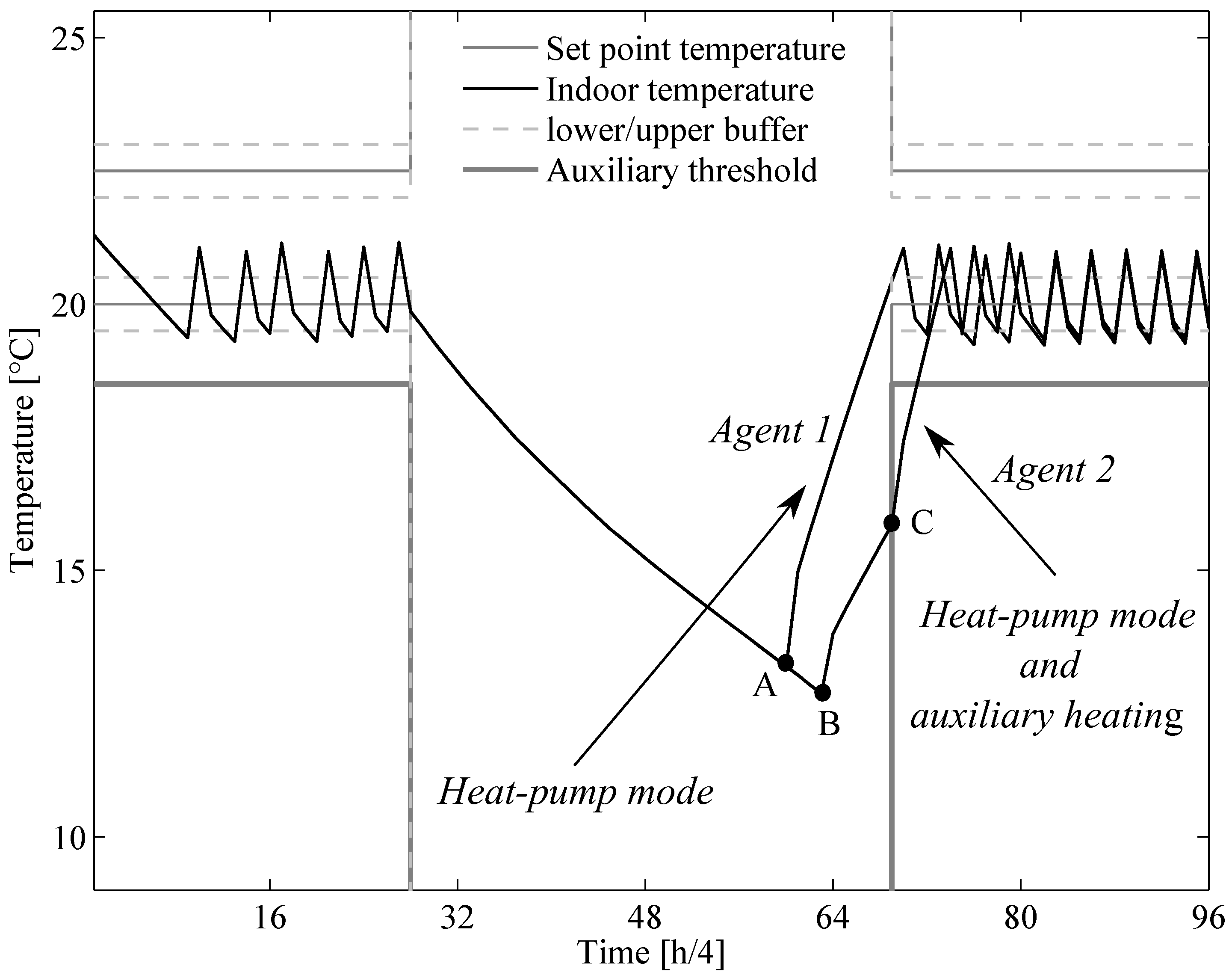
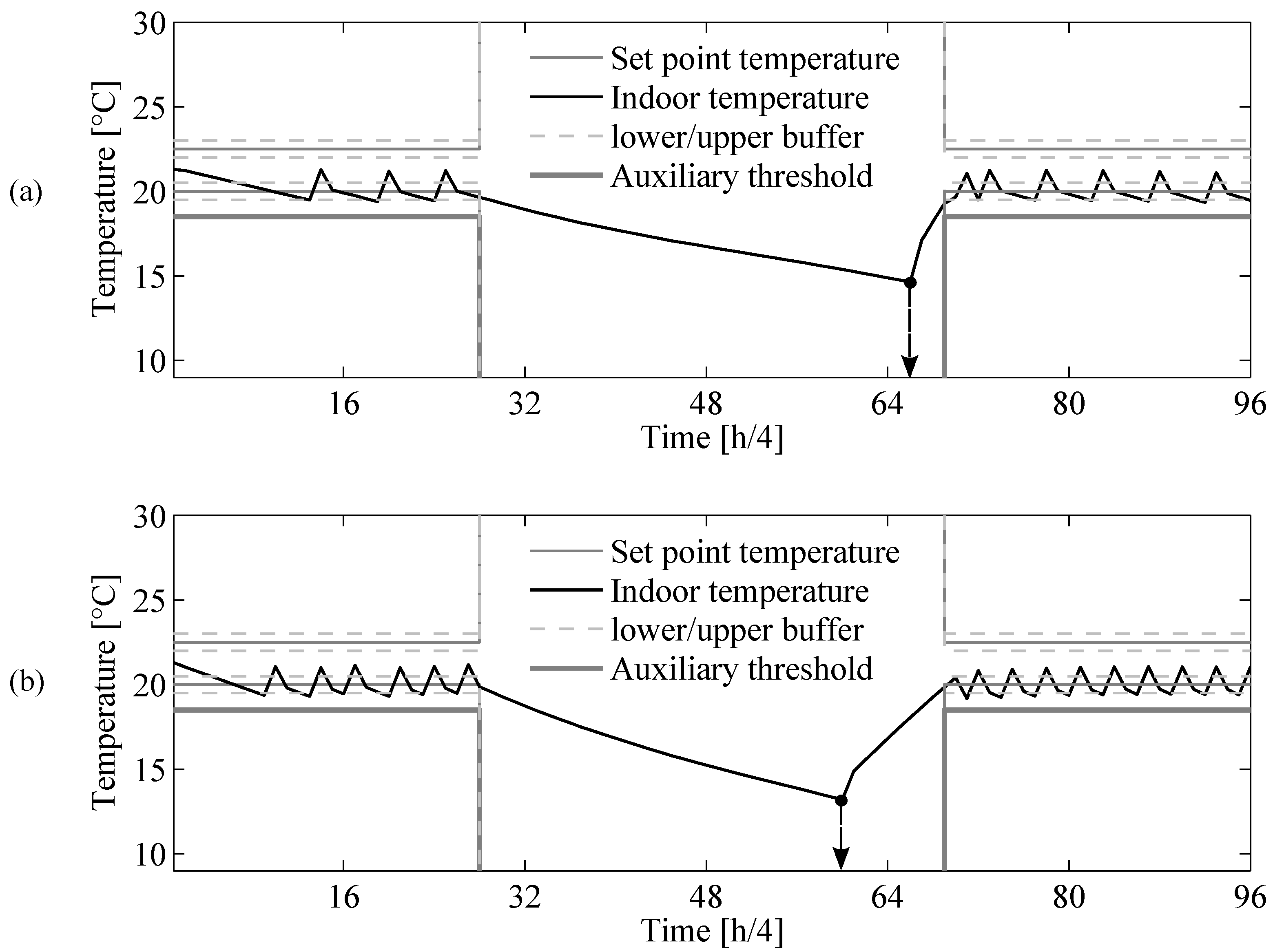
4.2. Thermostat Function

In order to guarantee the comfort of the end-user, the heat pump is equipped with a thermostat mechanism (Algorithm 2). The thermostat logic maps the requested control action $u_k$ taken in state ${\mathbf{x}}_k$ to a physical control action $u_k^{\mathrm{ph}}$:

$$u_k^{\mathrm{ph}}=T({\mathbf{x}}_k,u_k).$$

(8)

As such, the thermostat function T maps the requested control action to a physical quantity, which is required to calculate the cost value.

4.3. Augmented State

As previously stated, this paper assumes that the temperature of the building envelope cannot be measured. It is important to realize that the temperature of the building envelope contains essential information to accurately capture the transient response of the indoor air temperature. Moreover, the temperature of the building envelope represents information on the amount of thermal energy stored in the thermal mass of the building. A possible strategy is to represent the temperature of the building envelope by a handcrafted feature based on expert knowledge, which can be difficult to obtain for residential buildings. However, a more generic strategy is to include past observations of the state and action in the state variable [30,34]:

$${\mathbf{x}}_{\mathrm{aug},k}=(d,t,T_{\mathrm{in},k},{\mathbf{z}}_k,T_{\mathrm{out},k},S_k),$$

(9)

with:

$${\mathbf{z}}_k=(T_{\mathrm{in},k-1},...,T_{\mathrm{in},k-n},u_{k-1}^{\mathrm{ph}},...,u_{k-n}^{\mathrm{ph}}),$$

(10)

where n denotes the number of past observations of the indoor temperatures and physical actions. Note that the physical control actions have been included in the state, since they give an indication of the amount of energy added to the system. In the next section, a feature extraction technique is proposed to mitigate the “curse of dimensionality” [33] and to find a compact representation of the augmented state vector.

4.4. Transition Function

A detailed description of the transition function f that models the temperature dynamics of the building is given in Appendix B. This paper proposes a model-free approach and makes no assumption of the model type or its parameters.

4.5. Cost Function

The cost function $\rho :X\times U\to R$, associated with a single transition, is given by:

$$c_k=u_k^{\mathrm{ph}}\Delta t+{\alpha }_k,$$

(11)

where the parameter ${\alpha }_k$ represents a penalty for violating the comfort constraints and $\Delta t$ represent the time interval of one control period. When the indoor air temperature $T_{\mathrm{in}}$ is lower than ${\underset{\overline{}}{T}}_{\mathrm{s}}$ or higher than $\overline{T_{\mathrm{s}}}$, ${\alpha }_k$ is set to ${10}^5$ and otherwise zero.

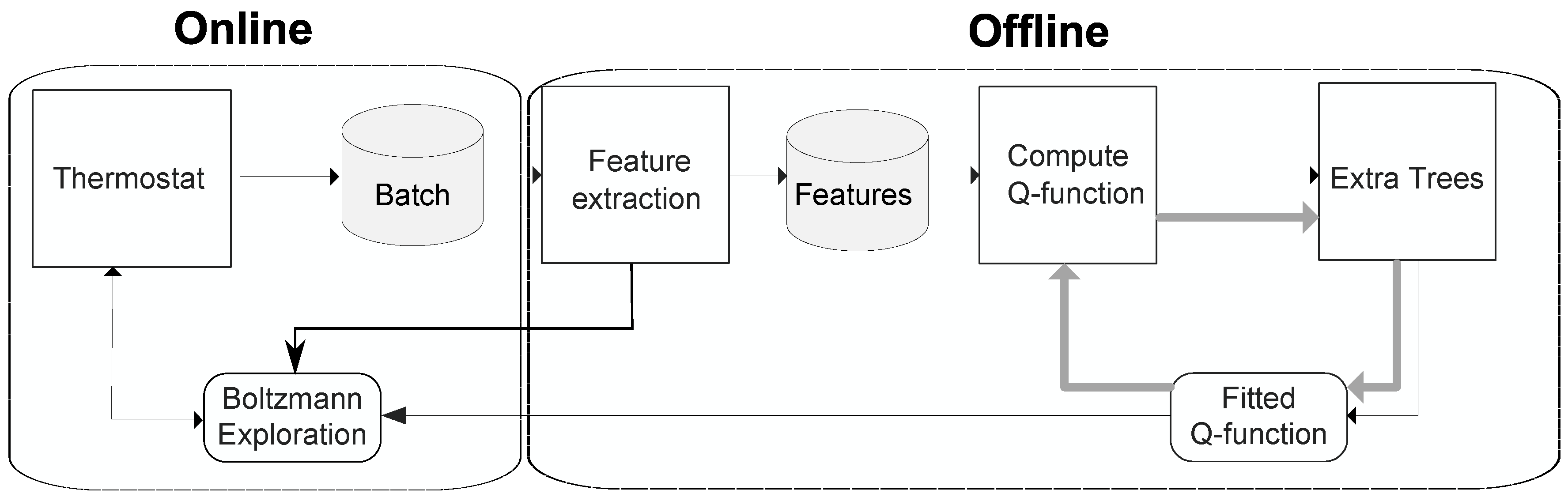
5. Model-Free Batch Reinforcement Learning Approach

Given full knowledge of the transition function, it can be possible to find an optimal policy by solving the Bellman Equation (6) for every state-action pair using techniques from approximate dynamic programming [17,33]. This paper, however, applies a model-free batch reinforcement learning technique, where the sole information available to solve the problem is the one obtained from daily observations of the following one-step transitions:

$$\mathcal{F}={\{({\mathbf{x}}_{\mathrm{aug},l},u_l,{\mathbf{x}}_{\mathrm{aug},l}^{\prime },u_l^{\mathrm{ph}})\}}_{l=1}^{\#\mathcal{F}},$$

(12)

where each tuple is made up of the augmented state ${\mathbf{x}}_{\mathrm{aug},l}$, the control action $u_l$, physical control action $u_l^{\mathrm{ph}}$ and its successor state ${\mathbf{x}}_{\mathrm{aug},l}^{\prime }$. Figure 3 outlines the building blocks of the model-free batch reinforcement learning method, which consists of two interconnected loops.

Figure 3. Online and offline loop of our proposed approach, which consists of a feature extraction (offline), fitted Q-iteration (offline) and Boltzmann exploration (online).

Figure 3. Online and offline loop of our proposed approach, which consists of a feature extraction (offline), fitted Q-iteration (offline) and Boltzmann exploration (online).

5.1. Offline Loop

The offline loop contains a feature extraction technique and a batch reinforcement learning method.

5.1.1. Feature Extraction

This paper proposes a feature extraction technique to find a low dimensional representation of the augmented state ${\mathbf{x}}_{\mathrm{aug},k}=(d,t,T_{\mathrm{in},k},{\mathbf{z}}_k,T_{\mathrm{out},k},S_k)$, by reducing the dimensionality of the state information corresponding to past observations:

$${\mathbf{z}}_{\mathrm{e},k}=\Phi ({\mathbf{z}}_k,W),$$

(13)

where $\Phi :Z\to Z_{\mathrm{e}}$ is a feature extraction function that maps $\mathbf{z}\in Z\subset R^p$ to the encoded state ${\mathbf{z}}_{\mathrm{e}}\in Z_{\mathrm{e}}\subset R^q$, with $q<p$ and where W contains the parameters corresponding to Φ.

This work introduces a feature extraction technique based on an auto-encoder. An auto-encoder or auto-associative neural network is an artificial neural network, with the same number of input as output neurons and a smaller number of hidden feature neurons. These hidden feature neurons function as a bottleneck and can be seen as a reduced representation of ${\mathbf{z}}_k$. During training of the auto-encoder, the output data are set to be equal to the input data. The weights of the network are then trained to minimize the squared error between the inputs and its reconstruction. Different training methods to find W can be found in the literature [35,36,37]. However, comparing the performance of these training methods is out of the scope of this paper. This work uses a hierarchical training strategy that uses a conjugate gradient descent method [38].

The next paragraph explains how a popular batch reinforcement learning technique, i.e., fitted Q-iteration, can be used, given:

$${\mathcal{F}}_{\mathcal{R}}={\{({\widehat{\mathbf{x}}}_{\mathrm{aug},l},u_l,{\widehat{\mathbf{x}}}_{\mathrm{aug},l+1},u_l^{\mathrm{ph}})\}}_{l=1}^{\#\mathcal{F}},$$

(14)

with:

$${\widehat{\mathbf{x}}}_{\mathrm{aug},l}=(d,t,T_{\mathrm{in},l},\Phi ({\mathbf{z}}_l,W),T_{\mathrm{out},l},S_l).$$

(15)

where ${\widehat{\mathbf{x}}}_{\mathrm{aug},l}$ denotes the reduced augmented state, and $\Phi ({\mathbf{z}}_l,W)$ denotes the encoded state information of the past observations ${\mathbf{z}}_l$.

5.1.2. Fitted Q-Iteration

Although other batch reinforcement learning techniques can be used, this work contributes to the application of fitted Q-iteration [24]. Fitted Q-iteration makes efficient use of gathered data and can be combined with different regression methods. In contrast to standard Q-learning [32], fitted Q-iteration computes the Q-function offline and makes use of the whole batch. An overview of the fitted Q-iteration algorithm is given in Algorithm 1. The algorithm iteratively builds a training set with all state-action pairs in ${\mathcal{F}}_{\mathcal{R}}$ as the input. The target values consist of the corresponding cost values and the optimal Q-value, based on the approximation of the previous iteration, for the next state. This works uses an extremely randomized tree ensemble method [39] to find an approximation $\widehat{Q}$ of the Q-function. The ensemble was set to 60 trees and a minimum of three samples for splitting a node. The number of samples selected at each node was set to the input dimension of the input space. More information on the regression method can be found in [39].

Algorithm 1 Fitted Q-iteration [24]

Input: ${\mathcal{F}}_{\mathcal{R}}={\{({\widehat{\mathbf{x}}}_{\mathrm{aug},l},u_l,{\widehat{\mathbf{x}}}_{\mathrm{aug},l+1},u_l^{\mathrm{ph}})\}}_{l=1}^{\#\mathcal{F}}$

1:  Initialize ${\widehat{Q}}_0$ to zero

2:  for $N=1,\dots ,T$ do

3:  for $l=1,\dots ,\#\mathcal{F}$ do

4:    $c_l=\rho ({\widehat{\mathbf{x}}}_{\mathrm{aug},l},u_l^{\mathrm{ph}})$

5:    $Q_{N,l}\leftarrow c_l+\underset{u\in U}{\text{min}}{\widehat{Q}}_{N-1,l}({\widehat{\mathbf{x}}}_{\mathrm{aug},l+1},u)$

6:  end for

7:  use regression to obtain ${\widehat{Q}}_N$ from $\left\{\left(({\widehat{\mathbf{x}}}_{\mathrm{aug},l},u_l),Q_{N,l}\right),l=1,\dots ,\#\mathcal{F}\right\}$

8:  end for

Output: $Q^{*}={\widehat{Q}}_N$

5.2. Online Loop

A Boltzmann exploration strategy [40] is used at each decision step to find the probability of selecting an action:

$$P\left(u|{\widehat{\mathbf{x}}}_{\mathrm{aug},k}\right)=\frac{e^{Q^{*}\left({\widehat{\mathbf{x}}}_{\mathrm{aug},k},u\right)/{\tau }_d}}{{\Sigma }_{u^{\prime }\in U}{e}^{Q^{*}\left({\widehat{\mathbf{x}}}_{\mathrm{aug},k},u^{\prime }\right)/{\tau }_d}},$$

(16)

where the parameter ${\tau }_d$ controls the amount of exploration and $Q^{*}$ is the Q-function obtained with Algorithm 1. The parameter ${\tau }_d$ is decreased during the simulation following a harmonic sequence [17]:

$${\tau }_d=\frac{1}{{\left(d\right)}^n},$$

(17)

where d denotes the current day and n is set to 0.7. Note that, if ${\tau }_d=0$, than the policy becomes greedy, and the best action is chosen.

6. Simulation Results

This section compares the performance of our learning agent to a default constant set-point strategy and a prescient set-back strategy.

6.1. Simulation Setup

The simulations use a second-order equivalent thermal parameter model to calculate the indoor air temperature and the envelope temperature of the building [41]. The parameters correspond to a building with a floor area of 200 ${\mathrm{m}}^2$ and a window-to-floor ratio of $30\%$. The model equations and parameters are presented in Appendix B. The building is equipped with a heat pump to satisfy the heating or cooling demand of the inhabitants. The heat pump can change its power set point every 15 min with 10 discrete heating or cooling actions. This paper considers two comfort settings, i.e., the default strategy and the set-back strategy. The default strategy has a constant temperature set point of 20.5 °C during the entire day. In contrast, the set-back strategy relaxes the set-point temperature from 7 to 17 h when the inhabitants are not present in the building.

The heat-pump thermostat is equipped with sensors to measure the outside temperature and solar irradiation, which are measurements obtained from a location in Belgium [42]. This work assumes that the heat-pump thermostat is provided with a forecast of the outside temperature and solar irradiation. However, internal heat gains caused by the inhabitants and electrical appliances cannot be measured or forecasted and are obtained from [43].

6.2. Learning Agent

The weights of the auto-encoder network are calculated at the beginning of each day and are used to calculate ${\mathcal{F}}_{\mathcal{R}}$. The state information corresponding to the past observations consists of the previous 10 indoor temperatures and the previous 10 control actions. The number of hidden neurons of the auto-encoder network is set to six. Given the batch ${\mathcal{F}}_{\mathcal{R}}$, the fitted Q-iteration algorithm constructs a Q-function for the next day (see Algorithm 1). This Q-function is then used online by the Boltzmann exploration strategy. Note that each simulation run begins with an empty batch of tuples and that observations of the previous day are daily added to ${\mathcal{F}}_{\mathcal{R}}$.

6.3. Prescient Method

The prescient set-back strategy assumes that the model parameters are known, and it has prescient knowledge on the outside temperature, solar irradiation and internal heat gains. A detailed description of the prescient method can be found in Appendix C. The outcome of the prescient set-back strategy is used to evaluate the performance of the learning agent and can be seen as an absolute lower-bound.

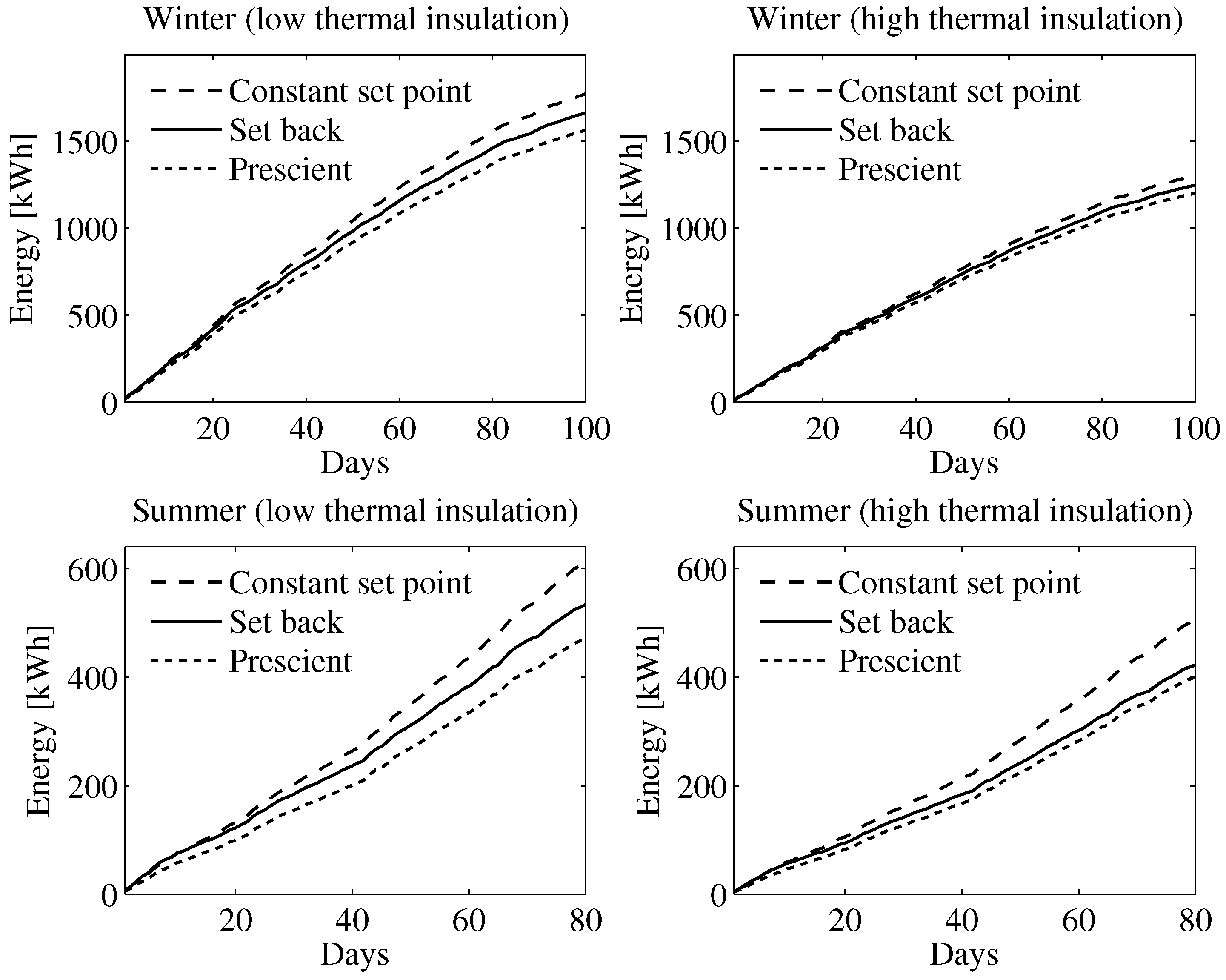
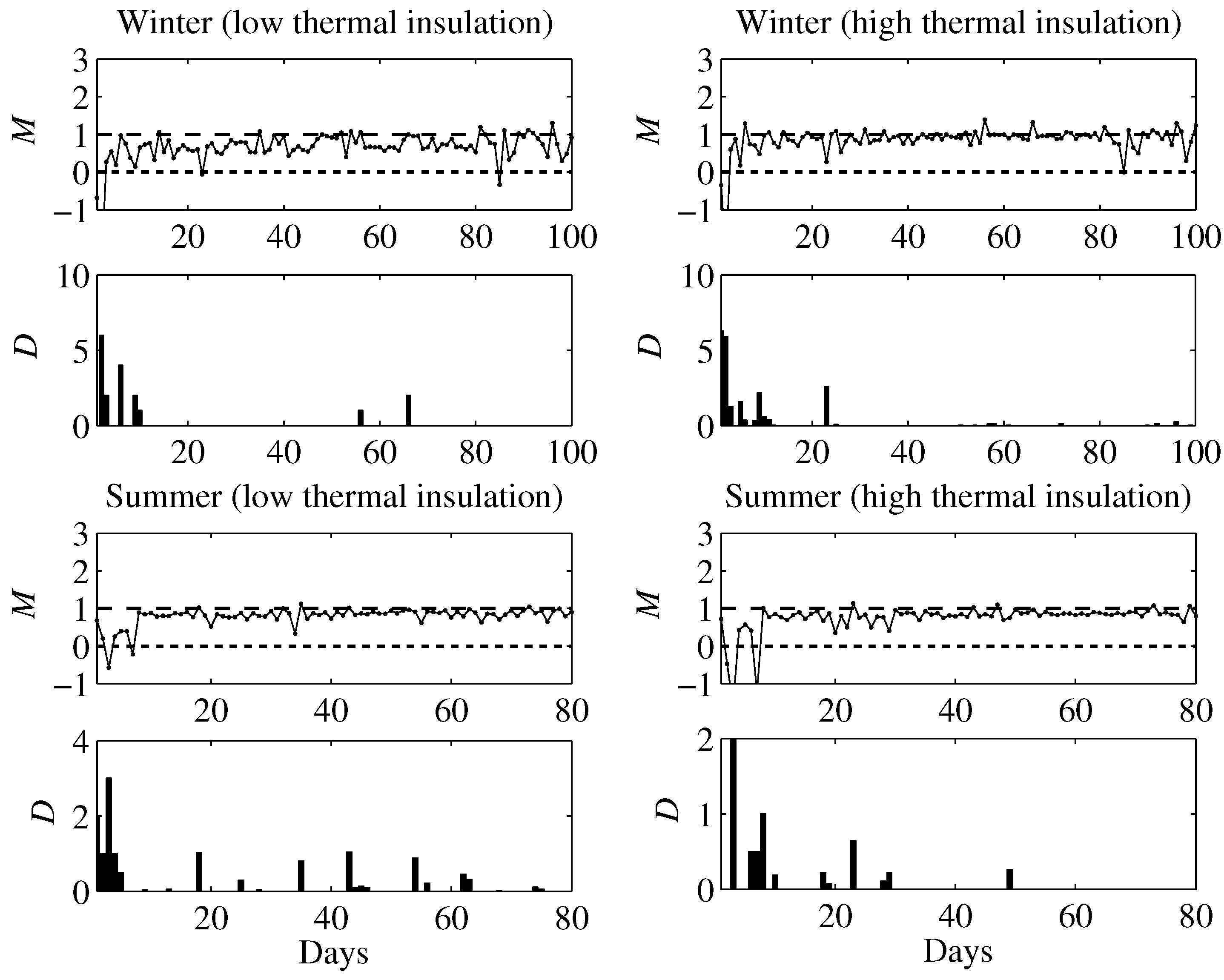
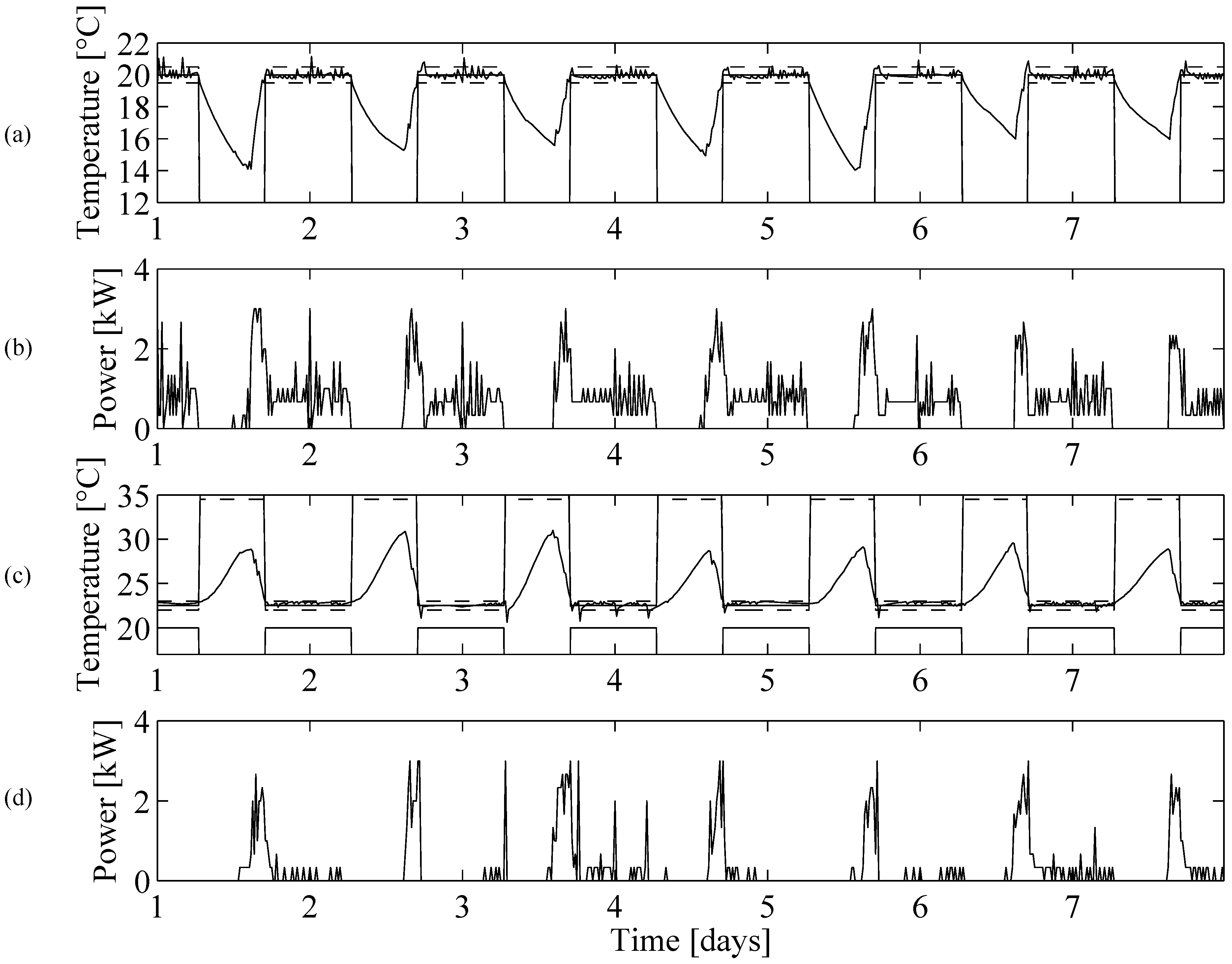
6.4. Simulation Results

The experiments compare the energy consumption and temperature violations of the learning agent with a set-back strategy, conventional constant set-point strategy and prescient set-back strategy. Note that the conventional constant temperature set point is the recommended strategy by the U.S. Department of Energy [6]. In order to examine the adaptability of the learning agent, an identical learning agent is applied to two building types, with a high and low thermal insulation level. The evaluation is repeated for 100 winter days (heating mode) and 80 summer days (cooling mode). Figure 4 depicts the cumulative energy consumption of the default controller, prescient controller and learning agent. As can be seen in Figure 4, the learning agent is able to reduce the total energy consumption compared to the default strategy for both building types. The simulation results indicate that the learning agent was able to reduce the energy consumption by 4%–9% during the winter and by 7%–11% during the summer. It should be noted, however, that the total energy consumption does not give a complete picture, as it does not consider the temperature violations. Remember that a comfort violation in the heating mode resulted in the activation of the less efficient auxiliary heating element. However, in the cooling mode, no auxiliary cooling is available. For this reason, Figure 5 shows the daily performance metric $M_d$ and the daily deviation $D_d$ between the temperature set point and the indoor temperature at 17 hour, which is the end of the set-back period. The daily deviation is calculated as follows:

$$D_d=\max (T_{\mathrm{in},17}-{\overline{T}}_{\mathrm{s},17},0)+\max ({\underset{\overline{}}{T}}_{\mathrm{s},17}-T_{\mathrm{in},17},0),$$

(18)

where $T_{\mathrm{in},17}$ is the indoor temperature at 17 h, and where ${\underset{\overline{}}{T}}_{\mathrm{s},17}$ and ${\overline{T}}_{\mathrm{s},17}$ are the minimum and maximum temperature set point at 17 h. The daily performance metric $M_d$ is calculated as follows:

$$M_d=\frac{e_{\mathrm{l}}-e_{\mathrm{d}}}{e_{\mathrm{p}}-e_{\mathrm{d}}},$$

(19)

where $e_{\mathrm{l}}$ denotes the daily energy consumption of the learning agent, $e_{\mathrm{d}}$ denotes the the daily energy consumption of the default strategy and $e_{\mathrm{p}}$ denotes the daily energy consumption of the prescient controller. As such, the metric M corresponds to zero if the learning agent obtains the same performance as the default strategy and corresponds to one if the learning agent obtains the same performance as the prescient controller. These figures show that the comfort violations decrease over the simulation horizon. At the same time, the performance metric M increases.

The results obtained with a mature controller (a batch size of 30 days) are depicted in Figure 6. Figure 6a and Figure 6b depict the indoor temperature and power consumption profile during seven winter days. Similarly, Figure 6c and Figure 6d depict the indoor temperature and power consumption during seven summer days. The simulation results indicate that the proposed learning agent can adapt itself to different building types and outside temperatures. In addition, the learning agent with a set-back strategy can reduce the energy consumption of a heat pump compared to the conventional constant temperature set-point strategy.

Figure 4. Cumulative energy plot of the default constant set-point strategy, our learning agent with a set-back strategy and a prescient set-back strategy.

Figure 4. Cumulative energy plot of the default constant set-point strategy, our learning agent with a set-back strategy and a prescient set-back strategy.

Figure 5. The performance metric M and the temperature violations D for the learning agent with a set-back strategy.

Figure 5. The performance metric M and the temperature violations D for the learning agent with a set-back strategy.

Figure 6. Indoor temperature and power consumption of the learning agent with set-back strategy during seven winter (a,b) and summer days (c,d).

Figure 6. Indoor temperature and power consumption of the learning agent with set-back strategy during seven winter (a,b) and summer days (c,d).

7. Conclusions and Future Work

This work addressed the challenge of developing a learning agent for a heat pump with a set-back strategy that saves energy compared to a constant temperature set-point strategy, which is recommended by the U.S. Department of Energy. To this end, this paper proposed an approach based on an auto-encoder and a popular model-free batch reinforcement learning technique, i.e., fitted Q-iteration. The auto-encoder is used to reduce the dimensionality of the state vector, which contains past observations of the indoor temperatures and energy consumptions. The performance of the set-back strategy has been evaluated for heating in the winter and cooling in the summer for two building types with different thermal characteristics. An equivalent thermal parameter model has been used to simulate the temperature dynamics of the indoor air temperature and the temperature of the building envelope. During the winter period, the set-back strategy was able to reduce the energy consumption 4%–9% compared to the default strategy. During the summer period, the set-back strategy saved 7%–11% compared to the default strategy. The results indicated that the proposed learning agent can adapt itself to different building types and weather conditions. The proposed learning agent obtained these results without making assumptions on the model or its parameters. As a result, the learning agents can be applied to virtually any building type.

With this work, we intended to show that model-free batch reinforcement learning techniques can provide a valuable alternative to model-based controllers. In our future work, we plan to focus on including real-time electricity prices in the objective and on implementing the presented approach in a lab environment.

References

1. U.S. Energy Information Administration (EIA). EIA Online Statistics. Available online: http://www.iea.org/topics/electricity/ (accessed on 21 May 2015).
2. Moretti, E.; Bonamente, E.; Buratti, C.; Cotana, F. Development of Innovative Heating and Cooling Systems Using Renewable Energy Sources for Non-Residential Buildings. Energies 2013, 6, 5114–5129. [Google Scholar] [CrossRef]
3. Luickx, P.J.; Peeters, L.F.; Helsen, L.M.; D’haeseleer, W.D. Influence of massive heat-pump introduction on the electricity-generation mix and the GHG effect: Belgian case study. Int. J. Energy Res. 2008, 32, 57–67. [Google Scholar] [CrossRef]
4. Forsén, M.; Boeswarth, R.; Dubuisson, X.; Sandström, B. Heat Pumps: Technology and Environmental Impact. 2005. Available online: http://ec.europa.eu/environment/ecolabel/about_ecolabel/reports/hp_tech_env_impact_aug2005.pdf (accessed on 31 July 2015).
5. Bayer, P.; Saner, D.; Bolay, S.; Rybach, L.; Blum, P. Greenhouse gas emission savings of ground source heat pump systems in Europe: A review. Renew. Sustain. Energy Rev. 2012, 16, 1256–1267. [Google Scholar] [CrossRef]
6. U.S. Department of Energy. Limitations for Homes with Heat Pumps, Electric Resistance Heating, Steam Heat, and Radiant Floor Heating. Available online: http://energy.gov/energysaver/articles/thermostats (accessed on 21 March 2015).
7. Michaud, N.; Megdal, L.; Baillargeon, P.; Acocella, C. Billing Analysis & Environment that “Re-Set” Savings for Programmable Thermostats in New Homes. 2009. Available online: http://www.anevaluation.com/pubs/090604_econoler_iepec_paper-lm.pdf (accessed on 31 July 2015).
8. Urieli, D.; Stone, P. A Learning Agent for Heat-pump Thermostat Control. In Proceedings of the 12th International Conference on Autonomous Agents and Multi-agent Systems (AAMAS), Saint Paul, MN, USA, 6–10 May 2013; pp. 1093–1100.
9. Rogers, A.; Maleki, S.; Ghosh, S.; Nicholas, R.J. Adaptive Home Heating Control Through Gaussian Process Prediction and Mathematical Programming. In Proceedings of the 2nd International Workshop on Agent Technology for Energy Systems (ATES), Taipei, Taiwan, 2–3 May 2011; pp. 71–78.
10. Nest Labs. The Nest Learning Thermostat. Available online: https://nest.com/ (accessed on 21 March 2015).
11. Honneywell. Programmable Thermostats. Available online: http://yourhome.honeywell.com/home/products/thermostats/ (accessed on 21 March 2015).
12. BuildingIQ. BuildingIQ, a Leading Energy Management Software Company. Available online: https://www.buildingiq.com/ (accessed on 21 March 2015).
13. Neurobat. Neurobat Interior Climate Technologies. Available online: http://www.neurobat.net/de/home/ (accessed on 21 March 2015).
14. Plugwise. Smart thermostat Anna. Available online: http://www.whoisanna.com/ (accessed on 21 March 2015).
15. Treado, S.; Chen, Y. Saving Building Energy through Advanced Control Strategies. Energies 2013, 6, 4769–4785. [Google Scholar] [CrossRef]
16. Cigler, J.; Gyalistras, D.; Širokỳ, J.; Tiet, V.; Ferkl, L. Beyond theory: The challenge of implementing Model Predictive Control in buildings. In Proceedings of the 11th REHVA World Congress (CLIMA), Prague, Czech Republic, 16–19 June 2013.
17. Powell, W. Approximate Dynamic Programming: Solving The Curses of Dimensionality, 2nd ed.; Wiley-Blackwell: Hoboken, NJ, USA, 2011. [Google Scholar]
18. Bertsekas, D. Dynamic Programming and Optimal Control; Athena Scientific: Belmont, MA, USA, 1995. [Google Scholar]
19. Morel, N.; Bauer, M.; El-Khoury, M.; Krauss, J. Neurobat, a predictive and adaptive heating control system using artificial neural networks. Int. J. Solar Energy 2001, 21, 161–201. [Google Scholar] [CrossRef]
20. Collotta, M.; Messineo, A.; Nicolosi, G.; Pau, G. A Dynamic Fuzzy Controller to Meet Thermal Comfort by Using Neural Network Forecasted Parameters as the Input. Energies 2014, 7, 4727–4756. [Google Scholar] [CrossRef]
21. Moon, J.W.; Chang, J.D.; Kim, S. Determining adaptability performance of artificial neural network-based thermal control logics for envelope conditions in residential buildings. Energies 2013, 6, 3548–3570. [Google Scholar] [CrossRef]
22. Henze, G.P.; Schoenmann, J. Evaluation of reinforcement learning control for thermal energy storage systems. HVACR Res. 2003, 9, 259–275. [Google Scholar] [CrossRef]
23. Wen, Z.; O Neill, D.; Maei, H. Optimal Demand Response Using Device-Based Reinforcement Learning. Available online: http://web.stanford.edu/class/ee292k/reports/ZhengWen.pdf (accessed on 27 July 2015).
24. Ernst, D.; Geurts, P.; Wehenkel, L. Tree-based batch mode reinforcement learning. J. Mach. Learn. Res. 2005, 6, 503–556. [Google Scholar]
25. Ernst, D.; Glavic, M.; Capitanescu, F.; Wehenkel, L. Reinforcement learning versus model predictive control: A comparison on a power system problem. IEEE Trans. Syst. Man Cybern. Syst. 2009, 39, 517–529. [Google Scholar] [CrossRef] [PubMed]
26. Lange, S.; Gabel, T.; Riedmiller, M. Batch Reinforcement Learning. In Reinforcement Learning: State-of-the-Art; Wiering, M., van Otterlo, M., Eds.; Springer: New York, NY, USA, 2012; pp. 45–73. [Google Scholar]
27. Claessens, B.; Vandael, S.; Ruelens, F.; de Craemer, K.; Beusen, B. Peak shaving of a heterogeneous cluster of residential flexibility carriers using reinforcement learning. In Proceedings of the 2nd IEEE Innovative Smart Grid Technologies Conference (ISGT Europe), Lyngby, Danish, 6–9 October 2013; pp. 1–5.
28. Ruelens, F.; Claessens, B.; Vandael, S.; Iacovella, S.; Vingerhoets, P.; Belmans, R. Demand Response of a Heterogeneous Cluster of Electric Water Heaters Using Batch Reinforcement learning. In Proceedings of the 18th IEEE Power System Computation Conference (PSCC), Wroclaw, Poland, 18–22 August 2014; pp. 1–8.
29. Lange, S.; Riedmiller, M. Deep auto-encoder neural networks in reinforcement learning. In Proceedings of the IEEE 2010 International Joint Conference on Neural Networks (IJCNN), Barcelona, Spain, 18–23 July 2010; pp. 1–8.
30. Mnih, V.; Kavukcuoglu, K.; Silver, D.; Graves, A.; Antonoglou, I.; Wierstra, D.; Riedmiller, M. Playing Atari with deep reinforcement learning. Available online: http://arxiv.org/pdf/1312.5602v1.pdf (accessed on 27 July 2015).
31. Riedmiller, M.; Gabel, T.; Hafner, R.; Lange, S. Reinforcement learning for robot soccer. Auton. Robots 2009, 27, 55–73. [Google Scholar] [CrossRef]
32. Sutton, R.S.; Barto, A.G. Reinforcement Learning: An Introduction; MIT Press: Cambridge, MA, USA, 1998. [Google Scholar]
33. Bellman, R. Dynamic Programming; Dover Publications, Inc.: New York, NY, USA, 2003. [Google Scholar]
34. Bertsekas, D.; Tsitsiklis, J. Neuro-Dynamic Programming; Athena Scientific: Nashua, NH, USA, 1996. [Google Scholar]
35. Hinton, G.E.; Salakhutdinov, R.R. Reducing the dimensionality of data with neural networks. Science 2006, 313, 504–507. [Google Scholar] [CrossRef] [PubMed]
36. Riedmiller, M.; Braun, H. A direct adaptive method for faster backpropagation learning: The RPROP algorithm. In Proceedings of the 1993 IEEE International Conference on Neural Networks, San Francisco, CA, USA, 28 March–1 April 1993; pp. 586–591.
37. Hestenes, M.R.; Stiefel, E. Methods of conjugate gradients for solving linear systems. J. Res. Natl. Bureau Stand. 1952, 49, 409–436. [Google Scholar] [CrossRef]
38. Scholz, M.; Vigário, R. Nonlinear PCA: A New Hierarchical Approach; ESANN: Bruges, Belgium, 2002; pp. 439–444. [Google Scholar]
39. Geurts, P.; Ernst, D.; Wehenkel, L. Extremely randomized trees. Mach. Learn. 2006, 63, 3–42. [Google Scholar] [CrossRef]
40. Kaelbling, L.P.; Littman, M.L.; Moore, A.W. Reinforcement learning: A survey. J. Artif. Intell. Res. 1996, 4, 237–285. [Google Scholar]
41. Chassin, D.; Schneider, K.; Gerkensmeyer, C. GridLAB-D: An open-source power systems modeling and simulation environment. In Proceedings of the IEEE Transmission and Distribution Conference and Exposition, Chicago, IL, USA, 21–24 April 2008; pp. 1–5.
42. Crawley, D.B.; Lawrie, L.K.; Winkelmann, F.C.; Buhl, W.F.; Huang, Y.J.; Pedersen, C.O.; Strand, R.K.; Liesen, R.J.; Fisher, D.E.; Witte, M.J.; et al. EnergyPlus: Creating a new-generation building energy simulation program. Energy Build. 2001, 33, 319–331. [Google Scholar] [CrossRef]
43. Dupont, B.; Vingerhoets, P.; Tant, P.; Vanthournout, K.; Cardinaels, W.; de Rybel, T.; Peeters, E.; Belmans, R. LINEAR breakthrough project: Large-scale implementation of smart grid technologies in distribution grids. In Proceedings of the 3rd IEEE PES Innovative Smart Grid Technologies Conference, (ISGT Europe), Berlin, Germany, 14–17 October 2012; pp. 1–8.
44. Sonderegger, R.C. Dynamic Models of House Heating Based on Equivalent Thermal Parameters. Ph.D. Thesis, Princeton University, Princeton, NJ, USA, 1978. [Google Scholar]
45. Klein, S.A. TRNSYS, a Transient System Simulation Program; Solar Energy Laboratory, University of Wisconsin: Madison, WI, USA, 1979. [Google Scholar]
46. Gurobi Optimization. Gurobi optimizer reference manual. Available online: http://www.gurobi. com (accessed on 21 March 2015).
47. Löfberg, J. YALMIP: A toolbox for modeling and optimization in MATLAB. In Proceedings of the IEEE 2004 International Symposium on Computer Aided Control Systems Design, Taipei, Taiwan, 2–4 September 2004; pp. 284–289.