
Optimal Energy Management of Multi-Microgrids with Sequentially Coordinated Operations


Abstract
:
1. Introduction
2. Proposed Optimal Energy Management of Cooperative Multi-Microgrids
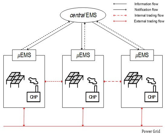
2.1. Cooperative Multi-Microgrid Community
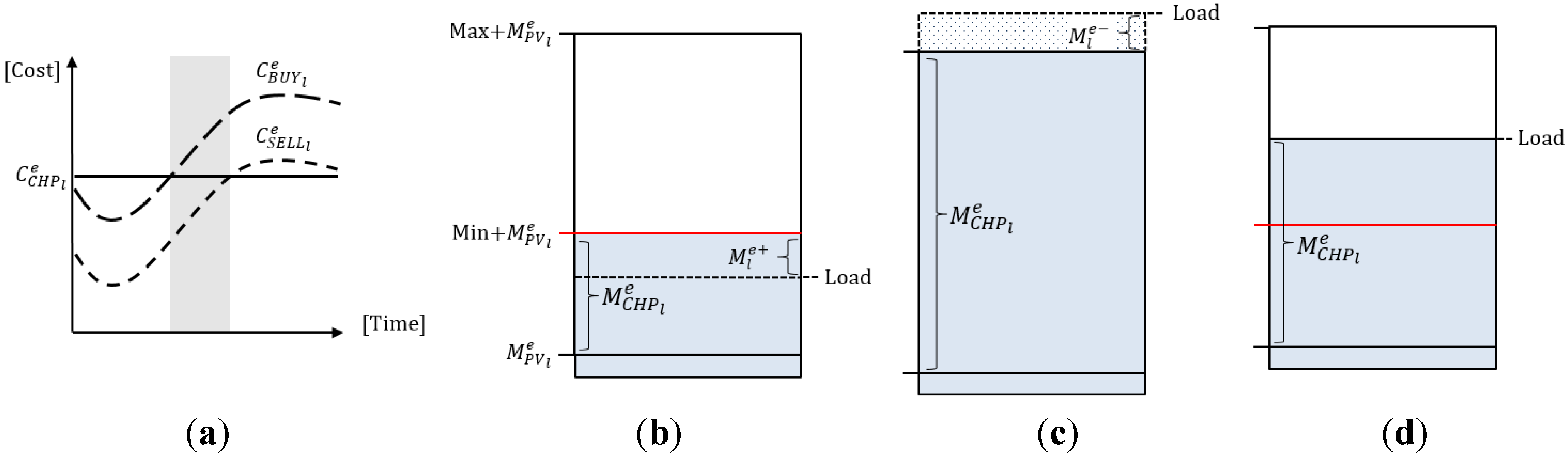
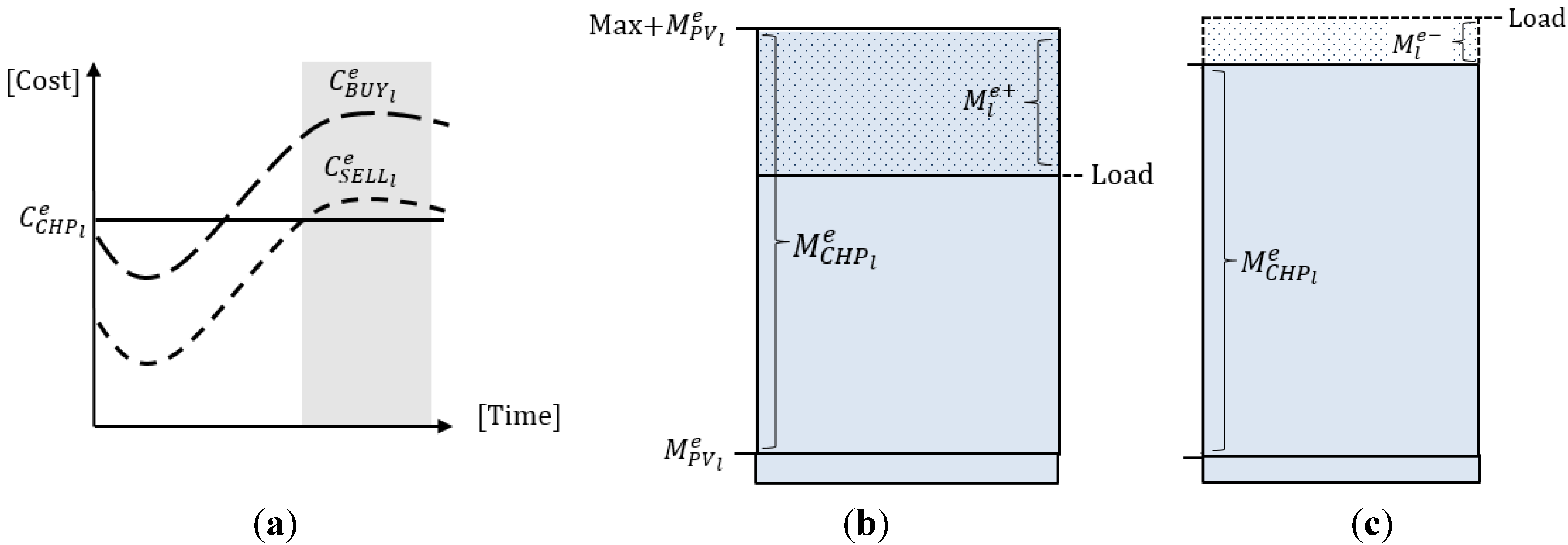
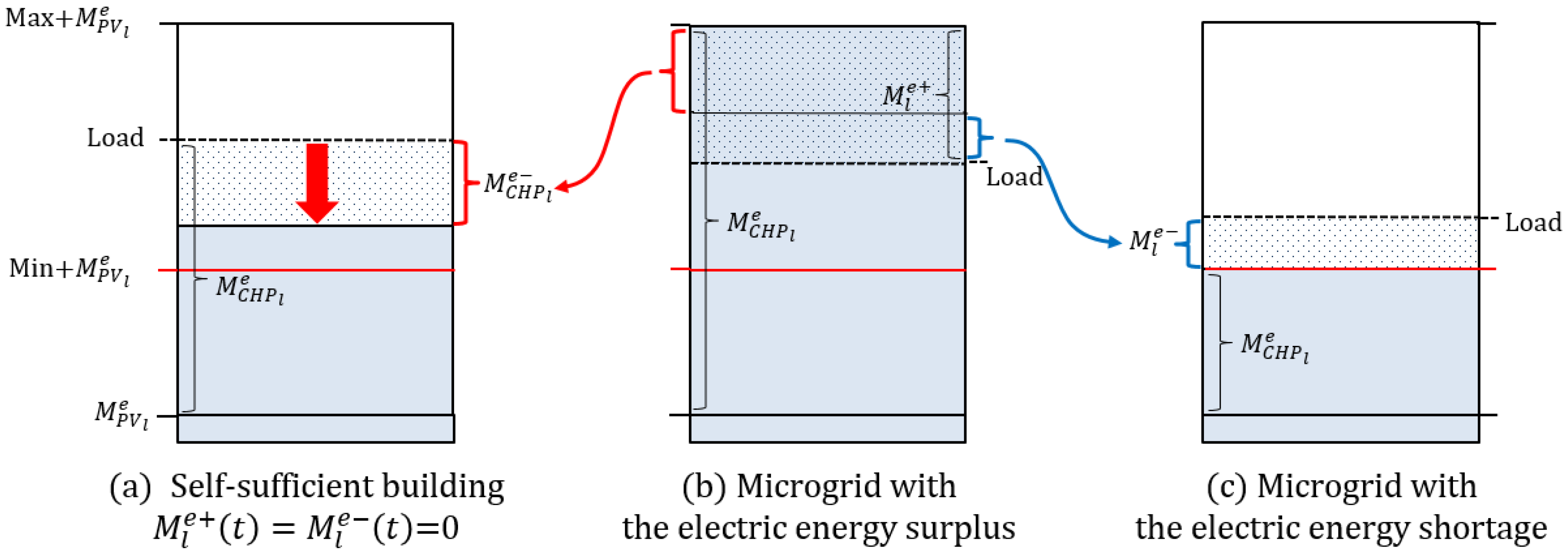
- Microgrids are equipped with photovoltaic (PV) systems and CHP generators as electric energy sources but the production costs of CHP generators are different;
- Microgrids can trade electric energy internally with other microgrids in the cooperative community as well as externally with the power grid;
- A μEMS in a microgrid is a centralized energy management system of its own microgrid;
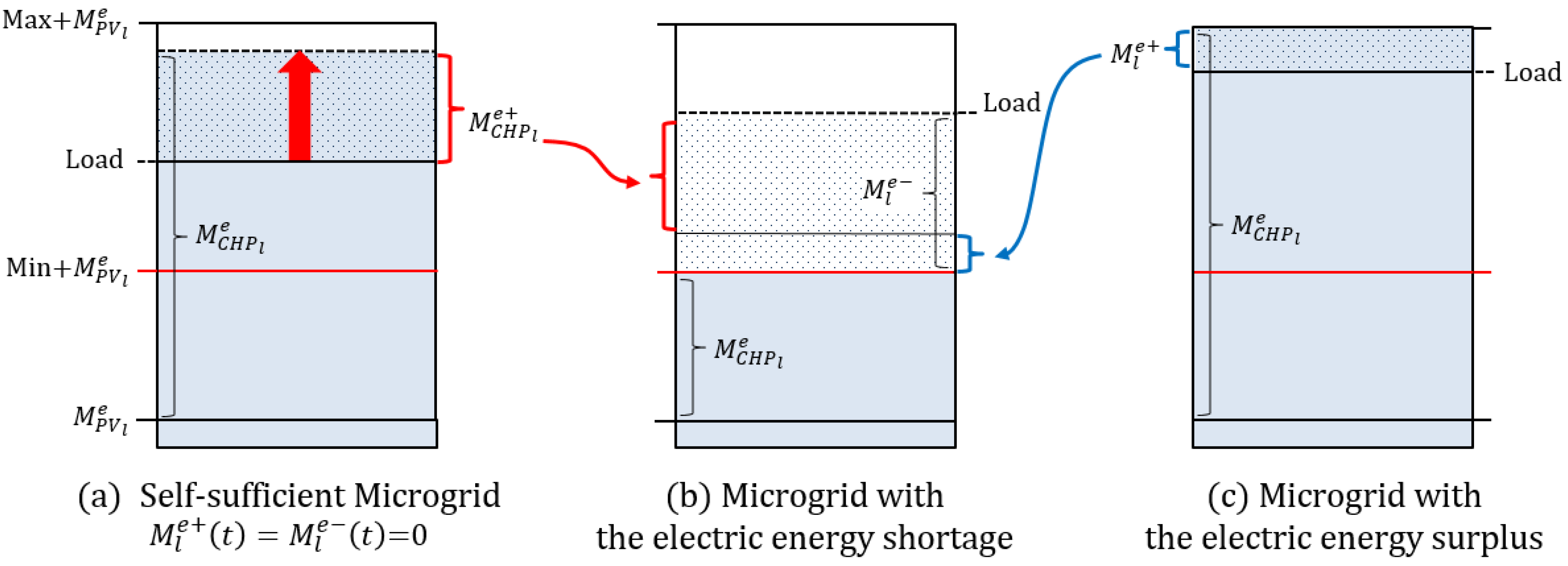
- A central energy management system (central EMS) has a global optimization function to manage any electric energy surplus/shortage of involved microgrids in the cooperative community.

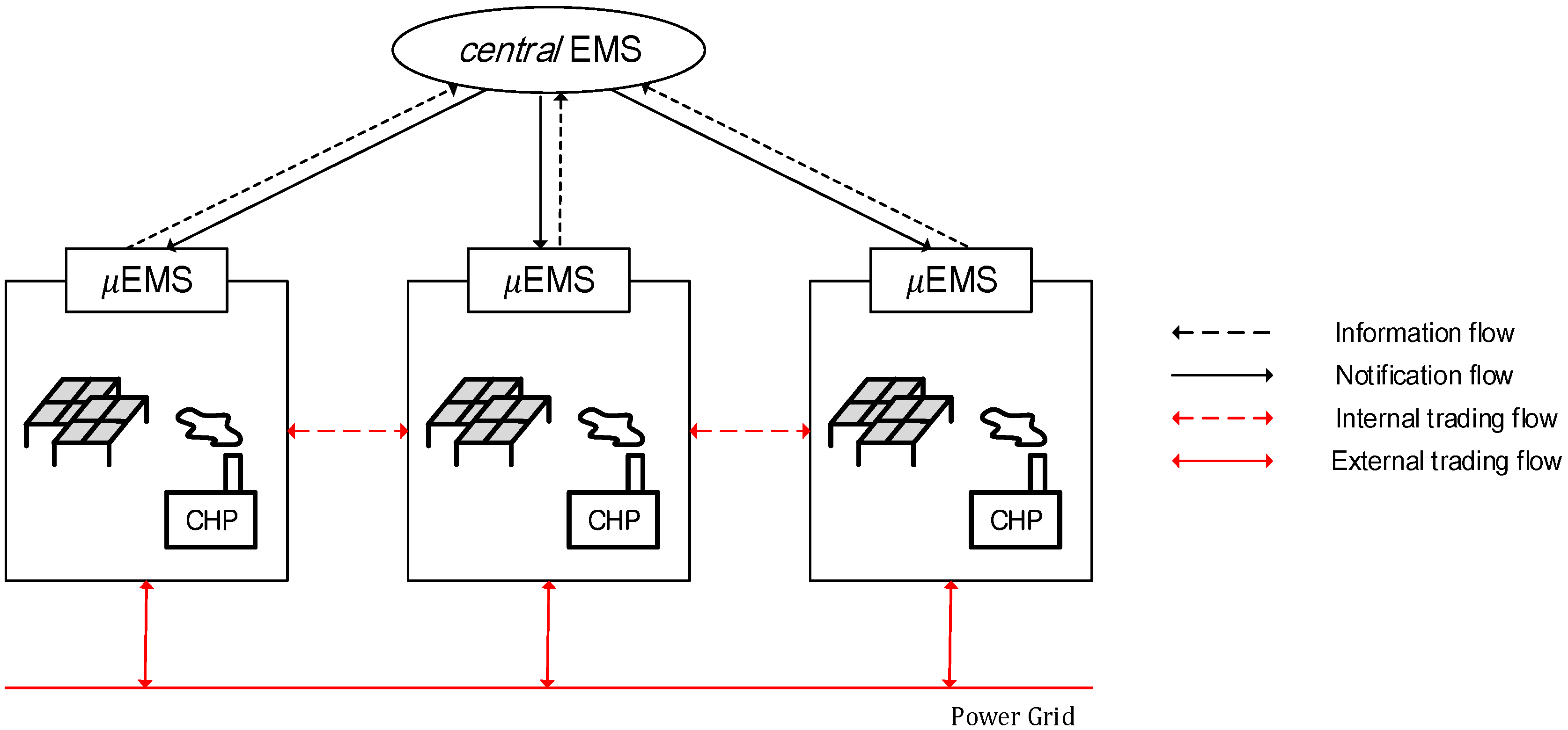
2.2. Sequentially Coordinated Operations of Cooperative Multi-Microgrids
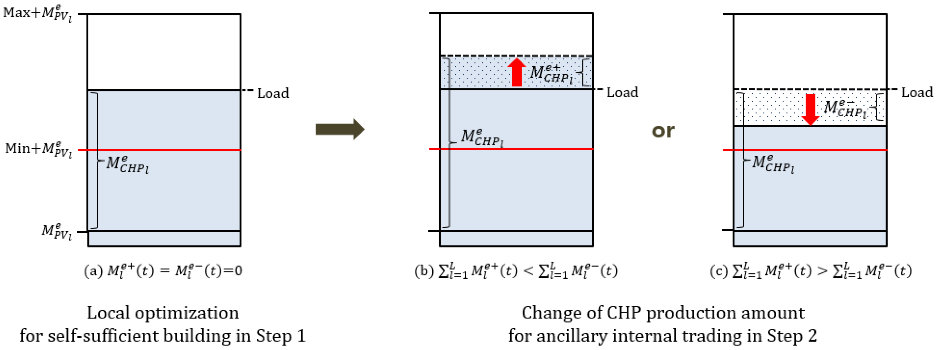
- Step 1: Local optimization of the electric energy by μEMS in each microgrid.
- Step 2: Global optimization of the electric energy cooperatively by central EMS in the cooperative community.

3. Mathematical Modeling of Cooperative Multi-Microgrid Operation Processes
3.1. Nomenclature
| ₩ | South Korea Won |
| t | the identifier of operation interval |
| T | the number of operation intervals |
| l | the identifier of microgrid |
| L | the number of microgrids |
| e | the identifier of electric energy |
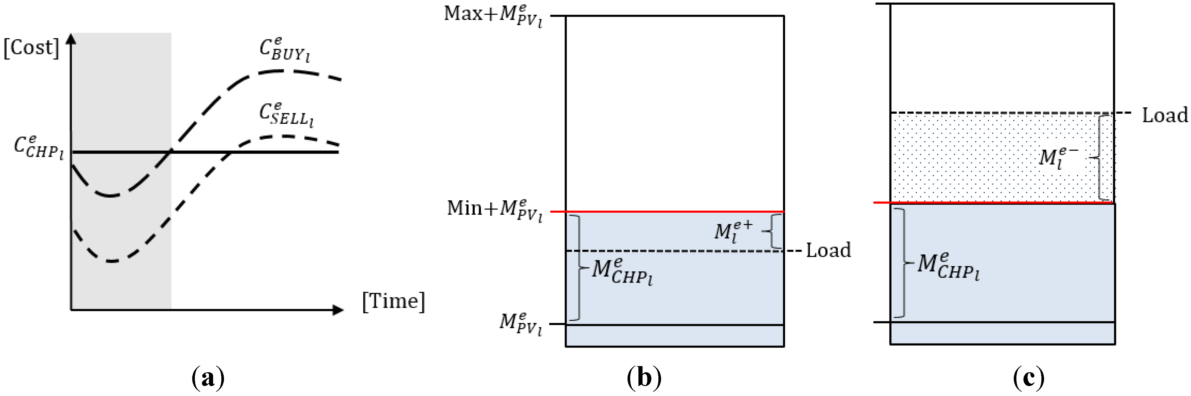
| the electric energy production cost of the PV in the lth microgrid (₩/kW h) | |
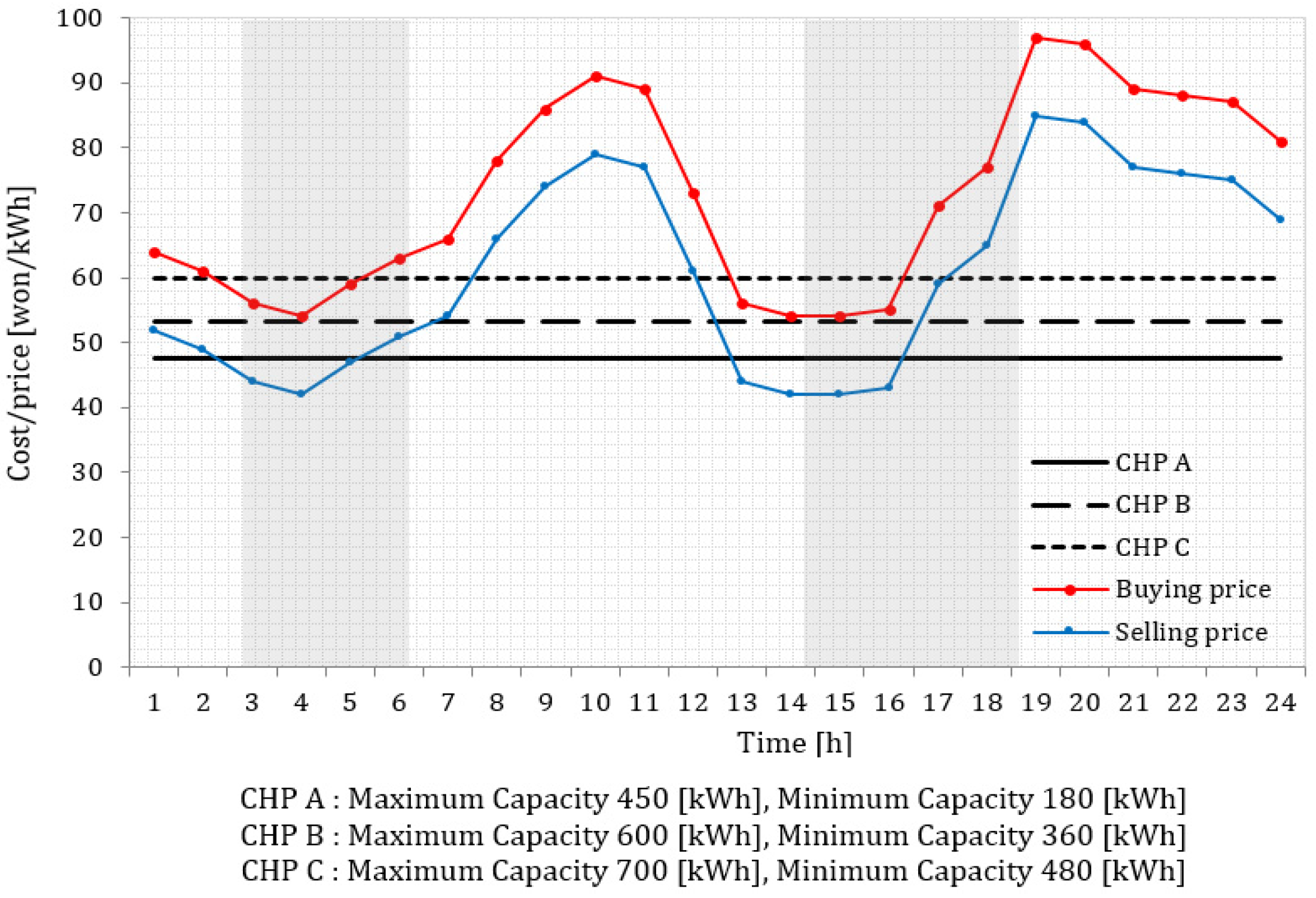
| the electric energy production cost of the CHP in the lth microgrid (₩) | |
| the buying price from the power grid in the lth microgrid at t (₩/kW h) | |
| the selling price to the power grid in the lth microgrid at t (₩/kW h] | |
| the amount of electric energy surplus in the lth microgrid at t (kW h) | |
| the amount of electric energy shortage in the lth microgrid at t (kW h) | |
| the output produced from the PV system in the lth microgrid at t (kW h) | |
| the electric energy production amount of the CHP in the lth microgrid at t (kW h) | |
| the electric energy demand in the lth microgrid at t (kW h) | |
| he amount of the selling electric energy in the lth microgrid determined by central EMS at t (kW h) | |
| the amount of the buying electric energy in the lth microgrid determined by central EMS at t (kW h) | |
| the sending electric energy amount in the lth microgrid at t (kW h) for the main internal trading (kW h) | |
| the received electric energy amount in the lth microgrid at t (kW h) for the main internal trading (kW h) | |
| the increased electric energy production amount of the CHP in the lth microgrid at t (kW h) for the ancillary internal trading (kW h) | |
| the decreased electric energy production amount of the CHP in the lth microgrid at t (kW h) for the ancillary internal trading (kW h) |
3.2. Mathematical Modeling of Step 1: Local Optimization


3.3. Mathematical Modeling of Step 2: Global Optimization


3.4. Total Optimal Operation Costs
4. Simulation Study


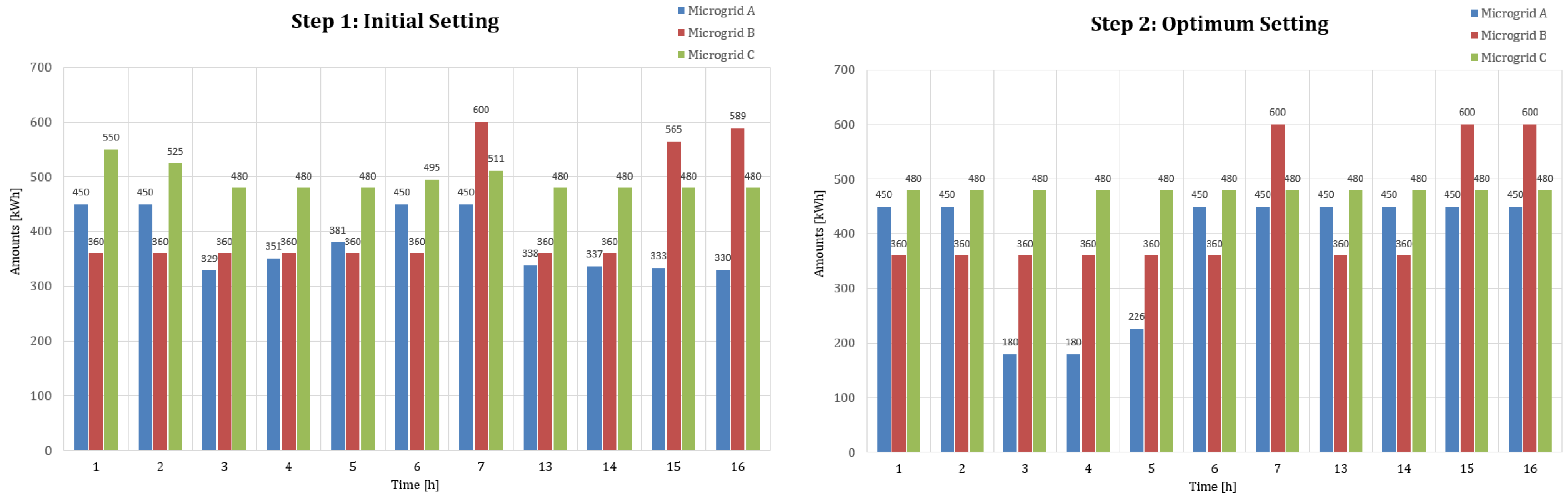
| Time | Microgrid A | Microgrid B | Microgrid C | ||||||||||||
|---|---|---|---|---|---|---|---|---|---|---|---|---|---|---|---|
| 1 | 369 | 450 | 0 | 81 | 0 | 192 | 360 | 0 | 168 | 0 | 550 | 550 | 0 | 0 | 0 |
| 2 | 345 | 450 | 0 | 105 | 0 | 187 | 360 | 0 | 173 | 0 | 525 | 525 | 0 | 0 | 0 |
| 3 | 329 | 329 | 0 | 0 | 0 | 189 | 360 | 0 | 171 | 0 | 475 | 480 | 0 | 5 | 0 |
| 4 | 351 | 351 | 0 | 0 | 0 | 188 | 360 | 0 | 172 | 0 | 472 | 480 | 0 | 8 | 0 |
| 5 | 381 | 381 | 0 | 0 | 0 | 200 | 360 | 0 | 160 | 0 | 485 | 480 | 0 | 0 | 5 |
| 6 | 372 | 450 | 0 | 78 | 0 | 224 | 360 | 0 | 136 | 0 | 495 | 495 | 0 | 0 | 0 |
| 7 | 470 | 450 | 0 | 0 | 20 | 247 | 600 | 0 | 353 | 0 | 511 | 511 | 0 | 0 | 0 |
| 8 | 454 | 450 | 6 | 2 | 0 | 305 | 600 | 0 | 295 | 0 | 568 | 700 | 7 | 139 | 0 |
| 9 | 363 | 450 | 9 | 96 | 0 | 535 | 600 | 0 | 65 | 0 | 620 | 700 | 10 | 90 | 0 |
| 10 | 371 | 450 | 10 | 89 | 0 | 673 | 600 | 5 | 0 | 68 | 651 | 700 | 12 | 61 | 0 |
| 11 | 373 | 450 | 13 | 90 | 0 | 670 | 600 | 8 | 0 | 62 | 682 | 700 | 16 | 34 | 0 |
| 12 | 416 | 450 | 18 | 52 | 0 | 651 | 600 | 10 | 0 | 41 | 729 | 700 | 25 | 0 | 4 |
| 13 | 361 | 338 | 23 | 0 | 0 | 320 | 360 | 15 | 55 | 0 | 743 | 480 | 28 | 0 | 235 |
| 14 | 362 | 337 | 25 | 0 | 0 | 343 | 360 | 19 | 36 | 0 | 762 | 480 | 24 | 0 | 258 |
| 15 | 357 | 333 | 24 | 0 | 0 | 585 | 565 | 20 | 0 | 0 | 803 | 480 | 20 | 0 | 303 |
| 16 | 351 | 330 | 21 | 0 | 0 | 603 | 589 | 14 | 0 | 0 | 807 | 480 | 13 | 0 | 314 |
| 17 | 357 | 450 | 18 | 111 | 0 | 600 | 600 | 12 | 12 | 0 | 769 | 700 | 4 | 0 | 65 |
| 18 | 391 | 450 | 8 | 67 | 0 | 557 | 600 | 4 | 47 | 0 | 775 | 700 | 0 | 0 | 75 |
| 19 | 464 | 450 | 0 | 0 | 14 | 424 | 600 | 0 | 176 | 0 | 824 | 700 | 0 | 0 | 124 |
| 20 | 467 | 450 | 0 | 0 | 17 | 356 | 600 | 0 | 244 | 0 | 804 | 700 | 0 | 0 | 104 |
| 21 | 428 | 450 | 0 | 22 | 0 | 317 | 600 | 0 | 283 | 0 | 793 | 700 | 0 | 0 | 93 |
| 22 | 417 | 450 | 0 | 33 | 0 | 299 | 600 | 0 | 301 | 0 | 723 | 700 | 0 | 0 | 23 |
| 23 | 414 | 450 | 0 | 36 | 0 | 247 | 600 | 0 | 353 | 0 | 664 | 700 | 0 | 36 | 0 |
| 24 | 400 | 450 | 0 | 50 | 0 | 216 | 600 | 0 | 384 | 0 | 604 | 700 | 0 | 96 | 0 |
| Time | Microgrid A | Microgrid B | Microgrid C | |||||||||||||||
|---|---|---|---|---|---|---|---|---|---|---|---|---|---|---|---|---|---|---|
| 1 | 0 | 0 | 0 | 0 | 0 | 58.2289 | 0 | 0 | 0 | 0 | 0 | 120.771 | 0 | 0 | 0 | 75 | 0 | 0 |
| 2 | 0 | 0 | 0 | 0 | 0 | 88.0036 | 0 | 0 | 0 | 0 | 0 | 144.996 | 0 | 0 | 0 | 45 | 0 | 0 |
| 3 | 0 | 0 | 0 | 149 | 0 | 0 | 0 | 0 | 0 | 0 | 0 | 26.233 | 0 | 0 | 0 | 0 | 0 | 0.76705 |
| 4 | 0 | 0 | 0 | 171 | 0 | 0 | 0 | 0 | 0 | 0 | 0 | 8.6 | 0 | 0 | 0 | 0 | 0 | 0.4 |
| 5 | 0 | 0 | 0 | 155 | 0 | 0 | 5 | 0 | 0 | 0 | 0 | 0 | 0 | 5 | 0 | 0 | 0 | 0 |
| 6 | 0 | 0 | 0 | 0 | 0 | 72.5327 | 0 | 0 | 0 | 0 | 0 | 126.467 | 0 | 0 | 0 | 15 | 0 | 0 |
| 7 | 0 | 20 | 0 | 0 | 0 | 0 | 20 | 0 | 0 | 0 | 0 | 302 | 0 | 0 | 0 | 31 | 0 | 0 |
| 8 | 0 | 0 | 0 | 0 | 0 | 2 | 0 | 0 | 0 | 0 | 0 | 295 | 0 | 0 | 0 | 0 | 0 | 139 |
| 9 | 0 | 0 | 0 | 0 | 0 | 96 | 0 | 0 | 0 | 0 | 0 | 65 | 0 | 0 | 0 | 0 | 0 | 90 |
| 10 | 40.3467 | 0 | 0 | 0 | 0 | 48.6533 | 0 | 68 | 0 | 0 | 0 | 0 | 27.6533 | 0 | 0 | 0 | 0 | 33.3467 |
| 11 | 45 | 0 | 0 | 0 | 0 | 45 | 0 | 62 | 0 | 0 | 0 | 0 | 17 | 0 | 0 | 0 | 0 | 17 |
| 12 | 45 | 0 | 0 | 0 | 0 | 7 | 0 | 41 | 0 | 0 | 0 | 0 | 0 | 4 | 0 | 0 | 0 | 0 |
| 13 | 0 | 0 | 112 | 0 | 0 | 0 | 55 | 0 | 0 | 0 | 0 | 0 | 0 | 55 | 0 | 0 | 68 | 0 |
| 14 | 0 | 0 | 113 | 0 | 0 | 0 | 36 | 0 | 0 | 0 | 0 | 0 | 0 | 36 | 0 | 0 | 109 | 0 |
| 15 | 0 | 0 | 117 | 0 | 0 | 0 | 0 | 0 | 35 | 0 | 0 | 0 | 0 | 0 | 0 | 0 | 151 | 0 |
| 16 | 0 | 0 | 120 | 0 | 0 | 0 | 0 | 0 | 11 | 0 | 0 | 0 | 0 | 0 | 0 | 0 | 183 | 0 |
| 17 | 58.6585 | 0 | 0 | 0 | 0 | 52.3415 | 6.34146 | 0 | 0 | 0 | 0 | 5.65854 | 0 | 65 | 0 | 0 | 0 | 0 |
| 18 | 44.0789 | 0 | 0 | 0 | 0 | 22.9211 | 30.9211 | 0 | 0 | 0 | 0 | 16.0789 | 0 | 75 | 0 | 0 | 0 | 0 |
| 19 | 0 | 14 | 0 | 0 | 0 | 0 | 138 | 0 | 0 | 0 | 0 | 38 | 0 | 124 | 0 | 0 | 0 | 0 |
| 20 | 0 | 17 | 0 | 0 | 0 | 0 | 121 | 0 | 0 | 0 | 0 | 123 | 0 | 104 | 0 | 0 | 0 | 0 |
| 21 | 6.7082 | 0 | 0 | 0 | 0 | 15.2918 | 86.2918 | 0 | 0 | 0 | 0 | 196.708 | 0 | 93 | 0 | 0 | 0 | 0 |
| 22 | 2.27246 | 0 | 0 | 0 | 0 | 30.7275 | 20.7275 | 0 | 0 | 0 | 0 | 280.273 | 0 | 23 | 0 | 0 | 0 | 0 |
| 23 | 0 | 0 | 0 | 0 | 0 | 36 | 0 | 0 | 0 | 0 | 0 | 353 | 0 | 0 | 0 | 0 | 0 | 36 |
| 24 | 0 | 0 | 0 | 0 | 0 | 50 | 0 | 0 | 0 | 0 | 0 | 384 | 0 | 0 | 0 | 0 | 0 | 96 |

| Time | 1 | 2 | 3 | 4 | 5 | 6 | 7 | 8 | 9 | 10 | 11 | 12 |
| Main | 0 | 0 | 0 | 0 | 5 | 0 | 20 | 0 | 0 | 68 | 62 | 45 |
| Ancillary | 70 | 45 | 149 | 171 | 155 | 15 | 31 | 0 | 0 | 0 | 0 | 0 |
| Internal | 70 | 45 | 149 | 171 | 160 | 15 | 51 | 0 | 0 | 68 | 62 | 45 |
| Time | 13 | 14 | 15 | 16 | 17 | 18 | 19 | 20 | 21 | 22 | 23 | 24 |
| Main | 55 | 36 | 0 | 0 | 65 | 75 | 138 | 121 | 93 | 23 | 0 | 0 |
| Ancillary | 112 | 113 | 152 | 131 | 0 | 0 | 0 | 0 | 0 | 0 | 0 | 0 |
| Internal | 167 | 149 | 152 | 131 | 65 | 75 | 138 | 121 | 93 | 23. | 30 | 0 |
5. Conclusions
Acknowledgments
Author Contributions
Conflicts of Interest
References
- Marnay, C.; Bailey, O. The CERTS Microgrid and the Future of the Macrogrid. In Proceeding of the 2004 ACEEE Summer Study on Energy Efficiency in Buildings, Pacific Grove, CA, USA, 22–27 August 2004.
- Bullis, K. Microgrid keeps the power local, cheap, and reliable. MIT Technology Review; Cambridge, MA, USA; San Francisco, CA, USA, 23 July 2012. Available online: http://www.technologyreview.com/news/428533/microgrid-keeps-the-power-local-cheap-and-reliable/ (accessed on 23 July 2012).
- Kim, H.-M.; Kinoshita, T.; Shin, M.-C. A multiagent system for autonomous operation of islanded microgrids based on a power market environment. Energies 2010, 3, 1972–1990. [Google Scholar] [CrossRef]
- Lim, Y.; Kim, H.-M.; Kinoshita, T. Distributed load-shedding system for agent-based autonomous microgrid operations. Energies 2014, 7, 385–401. [Google Scholar] [CrossRef]
- Kim, H.-M.; Lim, Y.; Kinoshita, T. An intelligent multiagent system for autonomous microgrid operation. Energies 2012, 5, 3347–3362. [Google Scholar] [CrossRef]
- Ng, E.J.; EL-Shatshat, R.A. Multi-Microgrid Control Systems (MMCS). In Proceedings of the 2010 IEEE Power and Energy Society Gneral Meeting, Minneapolis, MN, USA, 25–29 July 2010; pp. 1–6.
- Yoo, C.-H.; Chung, I.-Y.; Lee, H.-J.; Hong, S.-S. Intelligent control of battery energy storage for multi-agent based microgrid energy management. Energies 2013, 6, 4956–4979. [Google Scholar] [CrossRef]
- Kuo, M.-T.; Lu, S.-D. Design and implementation of real-time intelligent control and structure based on multi-agent systems in microgrids. Energies 2013, 6, 6045–6059. [Google Scholar] [CrossRef]
- Vasiljevska, J.; Peças Lopes, J.A.; Matos, M.A. Microgrid Impact Assessment Using Multi Criteria Decision Aid Methods. In Proceedings of the IEEE Bucharest 2009 PowerTech, Bucharest, Romania, 28 June–2 July 2009; pp. 1–8.
- Nguyen, T.A.; Mariesa, L.C. Optimization in Energy and Power Management for Renewable-Diesel Microgrids Using Dynamic Programming Algorithm. In Proceedings of the 2012 IEEE International Conference on Cyber Technology in Automation, Control, and Intelligent Systems (CYBER), Bangkok, Thailand, 27–31 May 2012; pp. 11–16.
- Chakraborty, S.; Simoes, M.G. PV-Microgrid Operational Cost Minimization by Neural Forecasting and Heuristic Optimization. In Proceedings of the 2008 IEEE Industry Applications Society Annual Meeting (IAS), Edmonton, AB, Canada, 5–9 October 2008; pp. 1–8.
- Chen, S.; Shroff, N.B.; Sinha, P. Energy Trading in the Smart Grid: from End-User’s Perspective. In Proceedings of the 2013 Asilomar Conference on Signals, Systems and Computers, Pacific Grove, CA, USA, 3–6 November 2013; pp. 327–331.
- Igualada, L.; Corchero, C.; Cruz-Zambrano, M.; Heredia, F.-J. Optimal energy management for a residential microgrid including a vehicle-to-grid system. IEEE Trans. Smart Grid 2014, 5, 2163–2172. [Google Scholar] [CrossRef]
- Chen, C.; Duan, S.; Cai, T.; Liu, B.; Yin, J. Energy Trading Model for Optimal Microgrid Scheduling Based on Genetic Algorithm. In Proceedings of the IEEE International Power Electronics and Motion Control 2009, Wuhan, China, 17–20 May 2009.
- Zhao, B.; Shi, Y.; Dong, X.; Laun, W.; Bornemann, J. Short-term operation scheduling in renewable-powered microgrids: A duality-based approach. IEEE Trans. Sustain. Energy 2014, 5, 209–217. [Google Scholar] [CrossRef]
- Khodaei, A. Resiliency-oriented microgrid optimal scheduling. IEEE Trans. Smart Grid 2014, 5, 1584–1591. [Google Scholar] [CrossRef]
- Bagherial, A.; Tafreshi, S.M.M. Developed Energy Management System for a Microgrid in the Competitive Electricity Market. In Proceedings of the IEEE PowerTech 2009, Bucharest, Romania, 28 June–2 July 2009.
- Nguyen, H.T.; Le, L.B. Optimal Energy Management for Building Microgrid with Constrained Renewable Energy Utilization. In Proceedings of the IEEE International Conference on Smart Grid Communications 2014, Venice, Italy, 3–6 November 2014.
- Chen, Y.-H.; Chen, Y.-H.; Hu, M.-C. Optimal Energy Management of Microgrid Systems in Taiwan. In Proceedings of the 2011 IEEE PES Innovative Smart Grid Technologies (ISGT), Hilton Anaheim, CA, USA, 17–19 January 2011; pp. 1–9.
- Kriett, P.O.; Salani, M. Optimal control of a residential microgrid. Energy 2012, 42, 321–330. [Google Scholar] [CrossRef]
- Rahbar, K.; Chai, C.C.; Zhang, R. Real-time energy management for cooperative microgrids with renewable energy integration. In Proceedings of the IEEE International Conference on Smart Grid Communications 2014, Venice, Italy, 3–6 November 2014.
- Nguyen, D.T.; Le, L.B. Optimal Energy Management for Cooperative Microgrids with Renewable Energy Resources. In Proceedings of the 2013 IEEE International Conference on Smart Grid Communications, Vancouver, BC, Canada, 21–24 October 2013; pp. 678–683.
© 2015 by the authors; licensee MDPI, Basel, Switzerland. This article is an open access article distributed under the terms and conditions of the Creative Commons Attribution license (http://creativecommons.org/licenses/by/4.0/).
Share and Cite
Song, N.-O.; Lee, J.-H.; Kim, H.-M.; Im, Y.H.; Lee, J.Y. Optimal Energy Management of Multi-Microgrids with Sequentially Coordinated Operations. Energies 2015, 8, 8371-8390. https://doi.org/10.3390/en8088371
Song N-O, Lee J-H, Kim H-M, Im YH, Lee JY. Optimal Energy Management of Multi-Microgrids with Sequentially Coordinated Operations. Energies. 2015; 8(8):8371-8390. https://doi.org/10.3390/en8088371
Chicago/Turabian StyleSong, Nah-Oak, Ji-Hye Lee, Hak-Man Kim, Yong Hoon Im, and Jae Yong Lee. 2015. "Optimal Energy Management of Multi-Microgrids with Sequentially Coordinated Operations" Energies 8, no. 8: 8371-8390. https://doi.org/10.3390/en8088371