Article

Optimal Coordinated Control of Power Extraction in LES of a Wind Farm with Entrance Effects

Department of Mechanical Engineering, University of Leuven, Celestijnenlaan 300A, Leuven B3001, Belgium
*
Author to whom correspondence should be addressed.
Energies 2016, 9(1), 29; https://doi.org/10.3390/en9010029
Submission received: 4 November 2015 / Revised: 24 December 2015 / Accepted: 29 December 2015 / Published: 6 January 2016
(This article belongs to the Collection Wind Turbines)

Abstract

:
We investigate the use of optimal coordinated control techniques in large eddy simulations of wind farm boundary layer interaction with the aim of increasing the total energy extraction in wind farms. The individual wind turbines are considered as flow actuators, and their energy extraction is dynamically regulated in time, so as to optimally influence the flow field. We extend earlier work on wind farm optimal control in the fully-developed regime (Goit and Meyers 2015, J. Fluid Mech. 768, 5–50) to a ‘finite’ wind farm case, in which entrance effects play an important role. For the optimal control, a receding horizon framework is employed in which turbine thrust coefficients are optimized in time and per turbine. Optimization is performed with a conjugate gradient method, where gradients of the cost functional are obtained using adjoint large eddy simulations. Overall, the energy extraction is increased 7% by the optimal control. This increase in energy extraction is related to faster wake recovery throughout the farm. For the first row of turbines, the optimal control increases turbulence levels and Reynolds stresses in the wake, leading to better wake mixing and an inflow velocity for the second row that is significantly higher than in the uncontrolled case. For downstream rows, the optimal control mainly enhances the sideways mean transport of momentum. This is different from earlier observations by Goit and Meyers (2015) in the fully-developed regime, where mainly vertical transport was enhanced.

1. Introduction

The size of wind farms has increased rapidly in recent years, and the power production of some of the largest farms is comparable to that of conventional power plants. The largest offshore wind farm to date is the 630-MW London Array with 175 turbines spread over an area of 100 km 2 . At these sizes, the efficiency of individual turbines in the wind farms differs considerably from that of a lone-standing turbine. It is well known that wake accumulation and the interaction of the wind farm with the atmospheric boundary layer lead to a decrease in energy extraction downstream in the farm that can amount up to 40% and more [1,2]. Moreover, increased turbulence intensities and wake meandering also lead to higher turbine loading. The current work investigates coordinated optimal control of wind turbines in a wind farm, focusing on improving energy extraction. To this end, large eddy simulations (LESs) of a wind farm boundary layer are performed, where the LES model itself is used as a control model in a receding horizon optimal control framework. Individual turbines are considered as flow actuators, whose energy extraction can be regulated dynamically in time and per turbine. Such an approach is infeasible as a real wind farm controller, as computational costs are prohibitive. Instead, the methodology is used as a means to explore the potential of coordinated control in wind farms, without excluding a priori any of the turbulent flow physics that could potentially improve performance. Recently, this approach was used by Goit and Meyers [3] for fully-developed ‘infinite’ wind farm boundary layers. In the current work, we extend this approach to a ‘finite’ farm in which entrance effects and boundary layer development play an important role.
In the past, studies on increasing energy extraction in wind farms have mainly focused on optimization of static power set-points of individual turbines throughout the farm. One of the first studies of this kind was performed by Steinbuch et al. [4] They proposed a concept of downrating the power output from upwind turbines in a farm, so that the wind speed in their wake would be higher, leading to higher energy extraction by downwind turbines and possibly an overall increase of power extraction. Later, many other studies followed this approach [5,6,7,8,9]. Unfortunately, in most of these studies, validation of the controllers in experiments or high fidelity turbulence-resolving flow simulations (such as LES) were impossible. Instead, simple wake engineering models were mostly used. Only recently, Gebraad [9] performed a detailed analysis using large eddy simulations, finding that static downrating of upstream turbines is not effective, as the reduction of wake deficit diffuses too much to be fully captured by the downstream turbines. Another static approach to increase energy extraction in wind farms is the use of non-zero yaw angles for turbines, redirecting their wake away from downstream turbines [10,11,12]. This approach has been shown to be successful both in experiments and in large eddy simulations. In the current work, however, our focus is not on yaw control.
Studies on dynamic control of turbine set points, in which turbine operational conditions are changed at a much faster rate, are more scarce. Most work in this area has focused on mitigation of turbine loads (see, e.g., [13,14]). A major challenge for increasing energy extraction is the formulation of fast enough control models that predict the complex high-dimensional interaction between control actions and the three-dimensional turbulent flow structures in the turbine wakes and in the atmospheric boundary layer. Due to the high dimensionality and complex physics of turbulent flows, such models currently do not exist. A number of model-free approaches to wind farm control have been considered recently [15,16,17,18], but for reasons of the convergence speed of the algorithm, a priori choices were required with respect to the structure and dimensionality of the controller. In fact, only relatively slow changes in turbine set points are practicable in such approaches. Moreover, to the authors knowledge, none of these methods were tested in experiments or in a high-fidelity simulation environment, such as LES, instead relying on simple wake accumulation models, such as the Jensen model [19].
The challenge in developing and evaluating dynamic wind farm control approaches is related to the very high dimensionality and complexity of the turbulent flow state with which the controls should interact. In addition, simulating the evolution of this turbulent flow state with large eddy simulations is very expensive. As a result, designing controllers based on intuition or simple first principle-based physical insights is nontrivial. The mixed successes of approaches as simple as the static set-point optimization discussed above illustrate this. In this context, Goit and Meyers [3] developed a method that allows one to explore optimal control actions in large parameter spaces taking into account the coupled interaction with the instantaneous turbulent motions. They found that energy extraction could be potentially increased by up to 16%. The main mechanism was related to improved wake recovery by increasing wake mixing and the vertical transport of energy. This was established for the limit of a fully-developed ‘infinite’ wind farm boundary layer [3]. In the current work, we extend the approach to a regular ‘finite’ wind farm, in which entrance effects in the first rows are expected to play an important role. Including entrance effects is of particular importance, since in the case of static set-point optimization (cf. the discussion above), it was shown that the potential of increased energy extraction in downstream rows does not compensate for the related losses due to downregulating the first row of turbines [9]. Finally, we remark that in the current work, we consider a wind farm optimal control study under neutral atmospheric conditions. On the simulation side, this is similar to many neutral wind farm simulation studies, such as, e.g., [20,21]. Note that wind farm performance is strongly influenced by stratification in the boundary layer and the atmosphere aloft (see, e.g., [22,23,24]), and these conditions can be potentially very interesting for an optimal control study. However, this is not in the scope of the current work.
The paper is further organized as follows. In Section 2, the governing flow equations and the optimal control framework are introduced. The optimization approach is also briefly discussed. Results are presented in Section 3, and optimized power output and time-averaged flow profiles are discussed. Finally, in Section 4, the main conclusions are presented.

2. Numerical Method

In Section 2.1, the governing equations for large eddy simulations are introduced, including implementation details on boundary conditions and wind turbines. Next, the optimal control approach and optimization method are presented in Section 2.2. Finally, the case set-up is discussed in Section 2.3.

2.1. Governing Flow Equations and Discretization

Large eddy simulations are performed in SP-Wind, an in-house research code that was developed in a series of earlier studies, wind farm simulations and flow optimization (see, e.g., [25,26,27]). The governing equations are the filtered incompressible Navier–Stokes equations for neutral flows and the continuity equation, i.e.,
· u ˜ = 0
u ˜ t + u ˜ · u ˜ = 1 ρ p ˜ + · τ M + f + λ ( x ) ( u ˜ in u ˜ )
where u ˜ = [ u ˜ 1 , u ˜ 2 , u ˜ 3 ] is the resolved velocity field, p ˜ is the pressure field, the term λ ( x ) ( u ˜ in u ˜ ) relates to our fringe-region implementation (cf. the further discussion below) and τ M is the subgrid-scale (SGS) model. We use a standard Smagorinsky model [28] with Mason and Thomson’s wall damping [29] to model the SGS stress. Furthermore, f represents the forces (per unit mass) introduced by the turbines on the flow. This turbine-induced force is modeled using an actuator-disk model (ADM) and is written for turbine i as:
f ( i ) = 1 2 C T , i V ^ i 2 R i ( x ) e i = 1 N t
where C T , i is the disk-based thrust coefficient. It should be noted that, unlike the conventional thrust coefficient C T , which is based on the undisturbed velocity far upstream of a turbine, C T , i is defined using the velocity at the turbine disk. It results from integrating lift and drag coefficients over the turbine blades, taking design geometry and flow angles into account (cf. Appendix A in [3] for a detailed formulation). Moreover, in an undisturbed uniform flow field, momentum theory can be employed to find C T = C T / ( 1 a ) 2 (cf., e.g., [30]). Further, V ^ i is the average axial flow velocity at the turbine rotor disk, obtained by disk averaging and time filtering the axial velocity at the turbine disk level, i.e., [3,27]:
V i ( t ) = 1 A Ω u ˜ ( x , t ) · e R i ( x ) d x , and d V ^ i d t = 1 τ ( V i V ^ i )
where we use τ = 5 s. In the above equations, e represents the unit vector perpendicular to the turbine disk, and R i ( x ) is a geometrical smoothing function that distributes the uniform surface force of the turbine over surrounding LES grid cells, with Ω R i ( x ) d x = A , where A is the turbine disk area. For more details regarding the implementation of the ADM in the SP-Wind code, the reader is referred to Meyers and Meneveau [27] and Goit and Meyers [3]. The total farm power, extracted by all turbines, can be expressed as:
P = Ω f · u ˜ d x = Ω i = 1 N t 1 2 C T , i V ^ i 2 u ˜ · e R i ( x ) d x = i = 1 N t 1 2 C T , i V ^ i 2 V i A
Finally, we remark that nowadays, other turbine models exist, such as the actuator line models (ALM). In particular, on sufficiently fine meshes, these allow a much finer description of the vortex dynamics in the near wake of the turbine (e.g., the effect of tip and root vortices, etc.). However, as shown in numerous studies, ADMs do provide a good description of the far wake dynamics and wake mixing, and the overall wind farm–boundary layer interaction (see, e.g., [31,32]). In view of the complexity of ALMs in an optimal control framework and the required high resolution (cf. also the discussion at the end of Section 4), we do not further consider them in the current study and focus on the use of the simpler ADM.
An overview of the computational domain is schematically shown in Figure 1. Inflow boundary conditions are used for the plane Γ 1 ; a classical high Reynolds number wall stress boundary condition is used on Γ 3 [33,34]; periodic boundary conditions are used for Γ 2 + and Γ 2 ; and a symmetry condition is used on Γ 3 + . SP-Wind uses a pseudo-spectral discretization in the horizontal directions. Therefore, the inflow boundary condition cannot be straightforwardly implemented as a Dirichlet condition. Instead, a fringe region technique [35] is used that smoothly forces the outflow region in the fringe region towards a desired inlet profile. To this end, we select:
λ ( x ) = λ max S x x s Δ s S x x e Δ e + 1
where:
S ( x ) = 0 x 0 , 1 / 1 + e 1 x 1 + 1 x 0 < x < 1 , 1 x 1 ,
with x s , x e the start and end of the fringe region and where Δ s , Δ e control the widths of the increase and decrease regions of the function λ ( x ) .
Figure 1. Computational domain with the fringe region.
Energies 09 00029 g001
The desired turbulent inflow field u ˜ in ( x , t ) is generated using a precursor method in which a separate simulation is performed, and stored to disk. This precursor simulation comprises a classical fully-developed boundary layer simulation (without a wind farm) that can be straightforwardly run on periodic domains. The method is visualized in Figure 2, showing velocity snapshots from the precursor boundary layer simulation and the main domain wind farm simulation, including the coupling from precursor simulation to the main domain fringe region.
Figure 2. Snapshots representing instantaneous streamwise velocity fields from the precursor boundary layer simulation (top) and from the finite farm simulation (bottom). The horizontal planes in the figures are taken at the hub height.
Energies 09 00029 g002
As mentioned above, SP-Wind uses a pseudo-spectral discretization in the horizontal directions, applying the 3 / 2 rule for dealiasing [36]. In the vertical direction, a fourth-order energy-conservative finite difference discretization scheme is used [37]. Mass is conserved by using a Poisson equation for the pressure that is solved using a direct solver. Finally, time integration is performed using a classical four-stage fourth-order Runge–Kutta scheme. For the simulations discussed in this paper, a fixed time step corresponding to a Courant–Friedrichs–Lewy (CFL) number of approximately 0.4 is used.

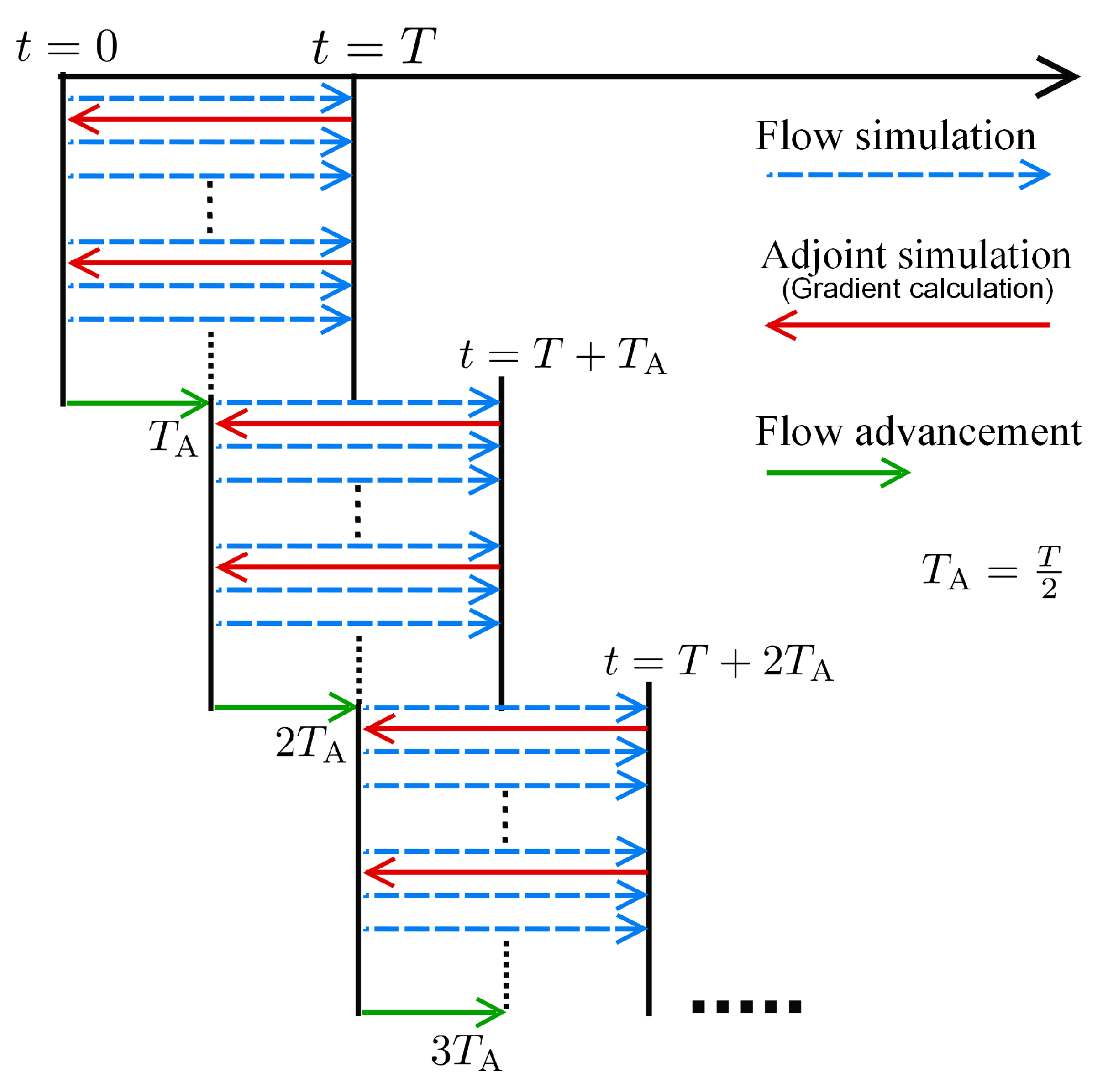
2.2. Optimal Control and Optimization Approach
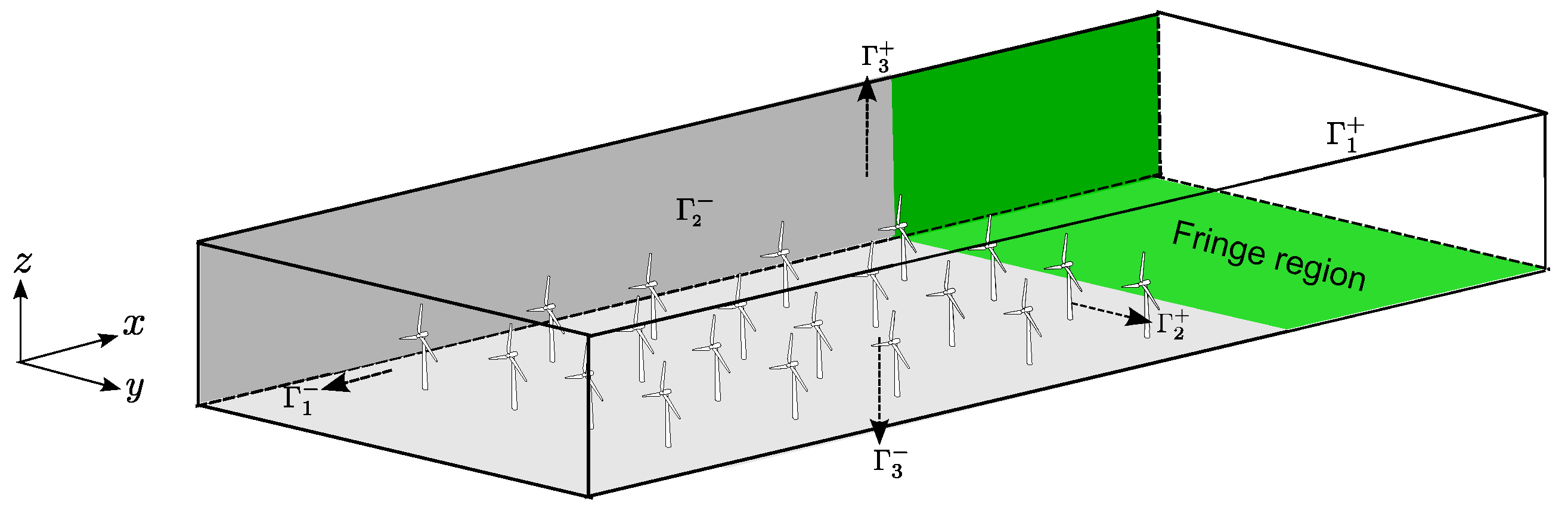
A classical receding horizon optimal control approach is employed for the control of wind farm boundary layer interaction. In this approach, a control time horizon T is selected, and the control parameters are optimized as a function of time over this control horizon given the full interaction with the turbulent flow field as described by the LES equations (cf. Figure 3). Here, the control parameters φ ( t ) correspond to all disk-based turbine thrust coefficients φ [ C T , 1 ( t ) , C T , 2 ( t ) , , C T , N t ( t ) ] in the control horizon. The optimization problem per time horizon is solved iteratively using a gradient-based approach (cf. further details below). Once an optimal set of controls is obtained, they are applied during a control time T A < T . Subsequently, a new optimization problem is formulated for the next time horizon, etc. In the current work, we use T A = T / 2 , similar to Goit and Meyers [3].
Figure 3. Schematic of the receding horizon optimal control approach.
Energies 09 00029 g003
For the optimization problem per time horizon, we aim at maximizing the total wind farm energy extraction. To this end, a cost functional is defined as:
J ( φ , q ) = 0 T P ( t ) d t = 0 T Ω f · u ˜ d x d t = 0 T Ω i = 1 N t 1 2 C T , i V ^ i 2 R i ( x ) u ˜ ( x , t ) · e d x d t = 0 T i = 1 N t 1 2 C T , i V ^ i 2 V i A d t
and where q [ u ˜ ( x , t ) , p ˜ ( x , t ) , V ^ ( t ) ] are the state variables corresponding to the LES velocity field, pressure field and the time-filtered turbine disk velocity fields. The optimization problem is then formulated in its reduced form [3], i.e.,
min φ J ˜ ( φ ) J ( φ , q ( φ ) )
where q ( φ ) is the solution to the state equations given the control inputs φ . This is obtained by solving the LES equations.
In order to solve Equation (9), a Polak–Ribière conjugate gradient method is used in combination with the Brent line search algorithm [38,39,40]. Implementation details are given in Delport, Baelmans and Meyers [26]. An important aspect of the algorithm is the determination of the gradient of the reduced cost functional J ˜ in the high-dimensional control space φ . To this end, the solution of the adjoint LES equations is required (cf. below), such that the gradient can be expressed as [3]:
J ˜ = 1 2 Ω V ^ 2 R ( x ) [ ( u ˜ + ξ ) · e ] d x
with R [ R 1 , , R N t ] and where ∘ is used to denote the entry-wise product (or Hadamard product), and V ^ 2 is the entry-wise square of V ^ . Furthermore, ξ ( x , t ) is the adjoint velocity field that is obtained by solving the adjoint equations. The derivation of the above relation is quite lengthy, but we refer the reader to [3] (Appendix C) for details.
The adjoint solution, required for the evaluation of Equation (10), is obtained by solving the following adjoint wind farm LES equations (cf. [3] for details of the derivation):
ξ t u ˜ · ξ ( ξ ) T · u ˜ = 1 ρ π + · τ M * + f * λ ( x ) ξ · ξ = 0 d χ i d t = 1 τ χ i + C T , i V ^ i Ω R i ( x ) ( u ˜ ξ ) · e d x , for i = 1 N t .
Here, ( ξ , π , χ ) are the adjoint variables associated with each state variable q = ( u ˜ , p ˜ , V ^ ) . Further, f * and τ M * are the adjoint forcing term and the adjoint of the SGS model, respectively. They are given by:
f * = i = 1 N t 1 2 C T , i V ^ i 2 + χ i A R i ( x ) e ,
τ M * = 2 s 2 2 S : S * ( 2 S : S ) 1 / 2 S + ( 2 S : S ) 1 / 2 S * ,
where S * = ( ξ + ( ξ ) T ) / 2 and S = ( u + ( u ) T ) / 2 .
Adjoint boundary conditions are similar to those of the forward problem. In the x and y directions, periodic boundary conditions are used. At Γ 3 + , a symmetry condition is imposed, while for Γ 3 , the adjoint of the high Reynolds number wall stress boundary condition is imposed (cf. [3] for details). Finally, Equation (11) slightly differs from the equations given in [3], i.e., an additional term λ ( x ) ξ appears, corresponding to the adjoint of the fringe forcing. The derivation of this term is trivial. The term dampens the outflow of the adjoint field at Γ 1 to an inflow ξ = 0 . This is fully equivalent to a standard system having non-periodicity with prescribed inflow at the upstream boundary and an outflow condition at the downstream boundary. A derivation of the adjoint boundary conditions for such a system yields a Dirichlet boundary condition for the adjoint velocity at the downstream boundary (with ξ = 0 ) and an outflow condition at the upstream boundary (see, e.g., [41]).
The adjoint equations show some similarity to the flow equations of the forward problem, e.g., time derivatives and convective terms can be recognized (albeit with different signs), continuity looks the same and there is also an adjoint pressure variable. Therefore, much of the discretization of the forward problem can be reused, with the same pseudo-spectral discretization in the horizontal directions, in combination with a fourth-order energy-conservative discretization in the vertical direction. For the time integration, a fourth-order Runge–Kutta method is also used. Due to the different signs of time and convective terms, the equations are solved backward in time, and the direction of the ‘adjoint’ flow is reversed. The adjoint equations themselves follow from a linearization of the governing equations around a state ( u ˜ , p ˜ , V ^ ) [3]. In the adjoint equations, this state is also required (cf. Equation (11)). To this end, the nonlinear forward problem is solved first, and the full space-time state is stored on disk. Subsequently, the state is used during the solution of the adjoint equations.
Details of the case set-up are summarized in Table 1. The domain size corresponds to L x × L y × H = 10 × 3 . 8 × 1 km 3 . The computational grid corresponds to N x × N y × N z = 384 × 256 × 200 , using 576 × 384 × 200 when applying the 3 / 2 dealiasing rule. The fringe region accounts for 15% of the streamwise length and is located at the downstream end of the domain, starting from x = 8 . 5 km. Fifty turbines with a diameter D = 100 m are arranged in a 10 × 5 matrix, with streamwise spacing S x = 7 D and spanwise spacing S y = 6 D . The selected resolution corresponds to typical cell sizes used in other wind farm simulations; in particular, it closely resembles the resolution of Case A3 in [30] and Case 1 in [42]. We refer the reader to these studies for a detailed grid sensitivity analysis.
Table 1. Summary of the simulation set-up for the optimal control of a finite farm.
Domain size L x × L y × H = 10 × 3 . 8 × 1 km 3
Fringe size L f 15 % of L x = 1 . 5 km
Fringe regionStart: 8.5 km; End: 10 km
Driving pressure gradient f = 4 × 10 4 m/s 2
Turbine dimensions D = 0 . 1 H = 100 m, z h = 0 . 1 H = 100 m
Turbine arrangement 10 × 5
Turbine spacing S x = 7 D , and S y = 6 D
Surface roughness z 0 = 10 4 H = 0 . 1 m
Grid size N x × N y × N z = 384 × 256 × 200
Cell size Δ x × Δ y × Δ z = 26 . 0 × 14 . 8 × 5 . 0 m 3
Time step0.6 s

2.3. Case Set-up

The distance between the last row of turbines and the start of the fringe region is set to 1.5 km (equivalent to 15D). The spanwise distance between the outer turbine columns and the (spanwise) domain boundaries corresponds to 7 D . This leads to a blockage of the wind farm frontal area to the total frontal area of the domain of around 9%. This could be further decreased by increasing the spanwise gap between the wind farm and the side boundaries, but in view of the huge computational resources required for the optimal-control study, this is not further explored in the current work. Note that the spanwise periodic boundary conditions do make our wind farm formally semi-infinite, i.e., only the streamwise direction is truly non-periodic, thus representing a farm that is finite in that direction. However, apart from the 9% blockage, we did further verify that the sideways wake expansion of the turbines in the side columns does not interfere with the spanwise boundary conditions along the length of the wind farm, so that our set-up is a reasonable approximation of a finite wind farm.
The inflow velocity is generated in a separate precursor boundary layer simulation, using the same domain size and grid resolution as those of the actual wind farm simulation (cf. Figure 2 and the discussion in Section 2.1). The precursor simulation is driven by a constant pressure gradient and has periodic boundary conditions in the horizontal directions. After an initial statistical convergence during which the flow evolves into a fully-developed turbulent boundary layer, the instantaneous velocity data in a region of a size equal to that of the fringe region of the main domain are written to files in every time step. These precursor data are read from the database and fed into the fringe region during the forward simulations in the optimization. The wind farm simulation is initialized with the converged precursor field and uses a spin-up period of approximately two through-flow time periods. Finally, note that during the iterations of the optimization, the same precursor data are needed multiple times, so that running the precursor simulation concurrently to the main simulation without the need of storing data on the disk (as, e.g., in the approach of Stevens et al. [43]) causes unnecessary computational overhead.
For the optimal control, we take a time horizon T = 240 s. This roughly corresponds to the time for the flow to pass four turbine rows, similar to the value used in [3]. The optimization algorithm is started with C T , i ( t ) = 2 . 0 (i.e., φ ( 0 ) = 2 . 0 ) for all turbines in the farm. This corresponds to the optimal operating condition of a lone-standing turbine following the Betz theory. To limit the computational cost, the optimization is not formally converged, but terminated after four conjugate gradient iterations. One conjugate gradient iteration requires roughly eight standard LES simulations (for the line search) and one adjoint LES for the determination of the gradient, leading to a total of 36 simulations per optimal control window. In total, 17 optimal control windows are performed, leading to a total control time of 17 T A = 2040 s and a total number of 612 simulations.
Similar to Goit and Meyers [3], we impose box constraints on the controls, i.e., 0 C T , i ( t ) 4 (these are trivially applied in the conjugate gradient algorithm). The lower constraint prevents the turbine from starting to operate as a fan, even if the optimization algorithm would ask for this. For the upper boundary, we do not a priori want to limit C T to the Betz limit ( C T = 2 ), but at the same time, we cannot leave it free, as C T is impractical from a turbine construction point of view. Therefore, we select an upper limit of C T = 4 . In a uniform steady flow, this corresponds to a turbine that maximizes the thrust force, leading to an axial induction factor a = 1 / 2 . In practice, this requires a turbine that is designed with a larger blade chord or a larger tip-speed ratio than is usually done for the Betz limit. For instance, using the “NREL offshore 5 MW wind turbine” [44] as a baseline, C T = 4 can be attained by a design with a double chord length, keeping all other aerodynamic parameters unchanged (cf. [3], Appendix A.2). We remark here that such a design may be economically not feasible, depending on the size of the potential gains of the optimal control in a wind farm. However, such an analysis is not in the scope of the current study.
An appreciation of a typical LES velocity field was already shown in Figure 2. Typical adjoint velocity fields are shown in Figure 4. Since the initial condition for the adjoint equation corresponds to ξ ( x , T ) = 0 , at T t = 22 s (Figure 4a), the field is largely zero (see the discussion in [3]). At T t = 22 s and T t = 70 s, it is observed that changes to the cost functional originate from tubes upstream of the rotors. In later snapshots (e.g., at time T t = 175 s, shown in Figure 4c) the tubes hit the upstream turbines, and the adjoint field becomes fully turbulent inside the farm. This indicates that the power generation in a wind farm is influenced by the interactions between the turbines, as well as by their interaction with the boundary layer. Finally, the role of the fringe region in the adjoint simulation is to suppress the upstream propagation of the field over the periodic boundary condition. This is clearly visible in Figure 4c. The adjoint field in the fringe region is almost zero, except for the very end of the domain, where the fringe function λ ( x ) is small. In this way, the interaction between the adjoint field developing upstream of the farm and the downstream turbines can be avoided, thereby imposing the non-periodicity in the streamwise direction.

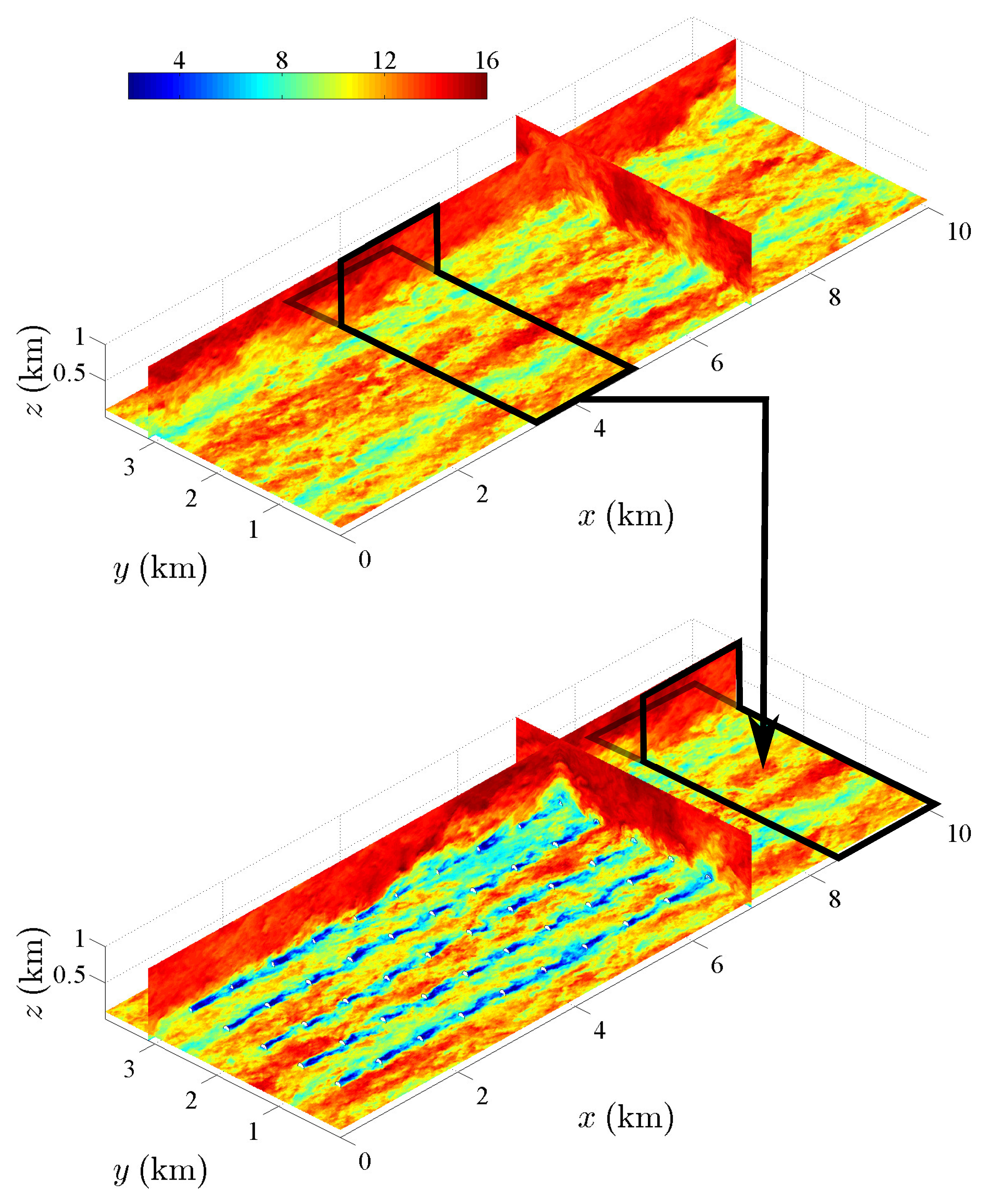
3. Results and Discussion

Results of the optimal control in a ‘finite’ wind farm are now presented, and differences or parallels to the fully-developed case of Goit and Meyers [3] are discussed.

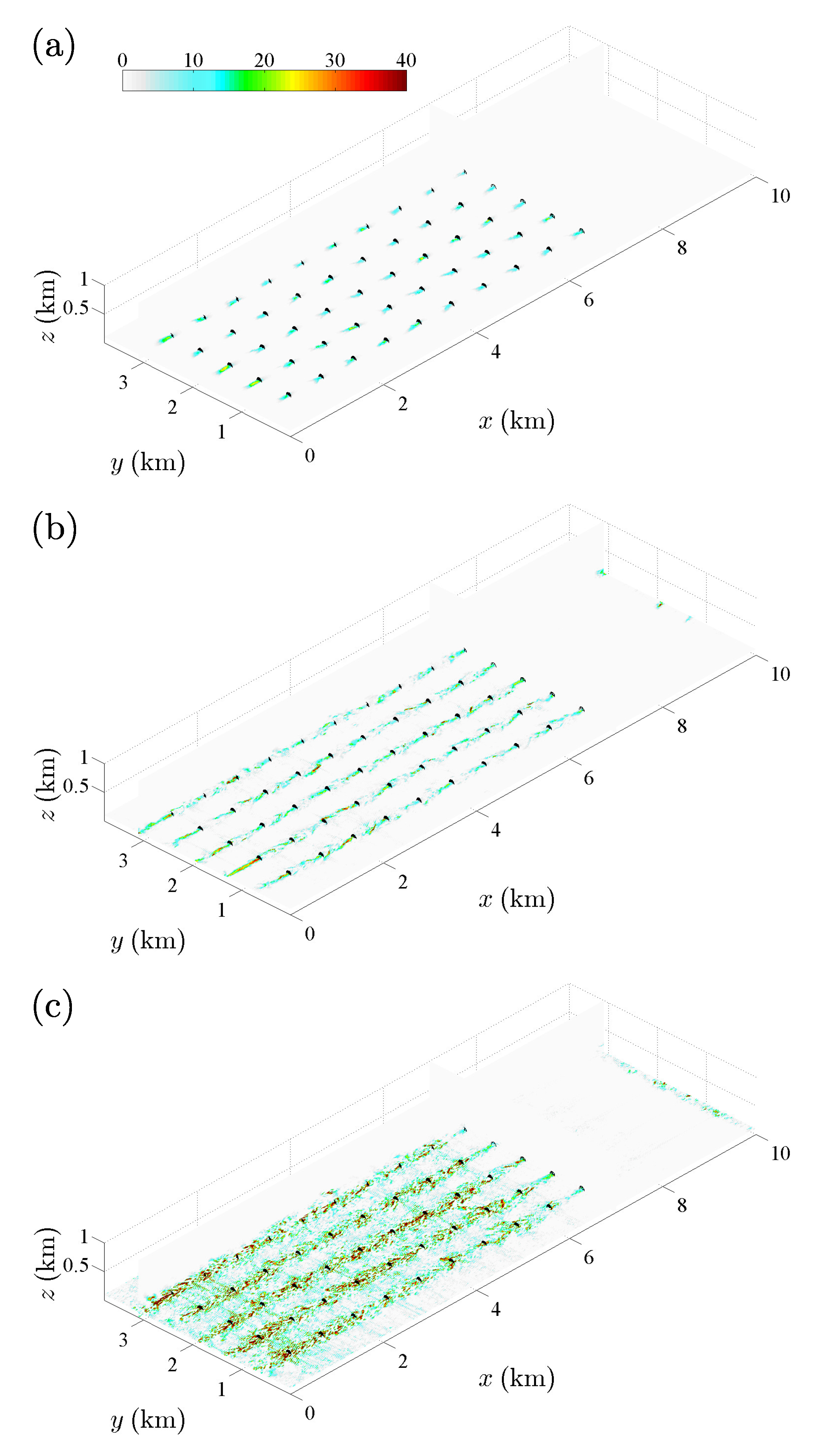
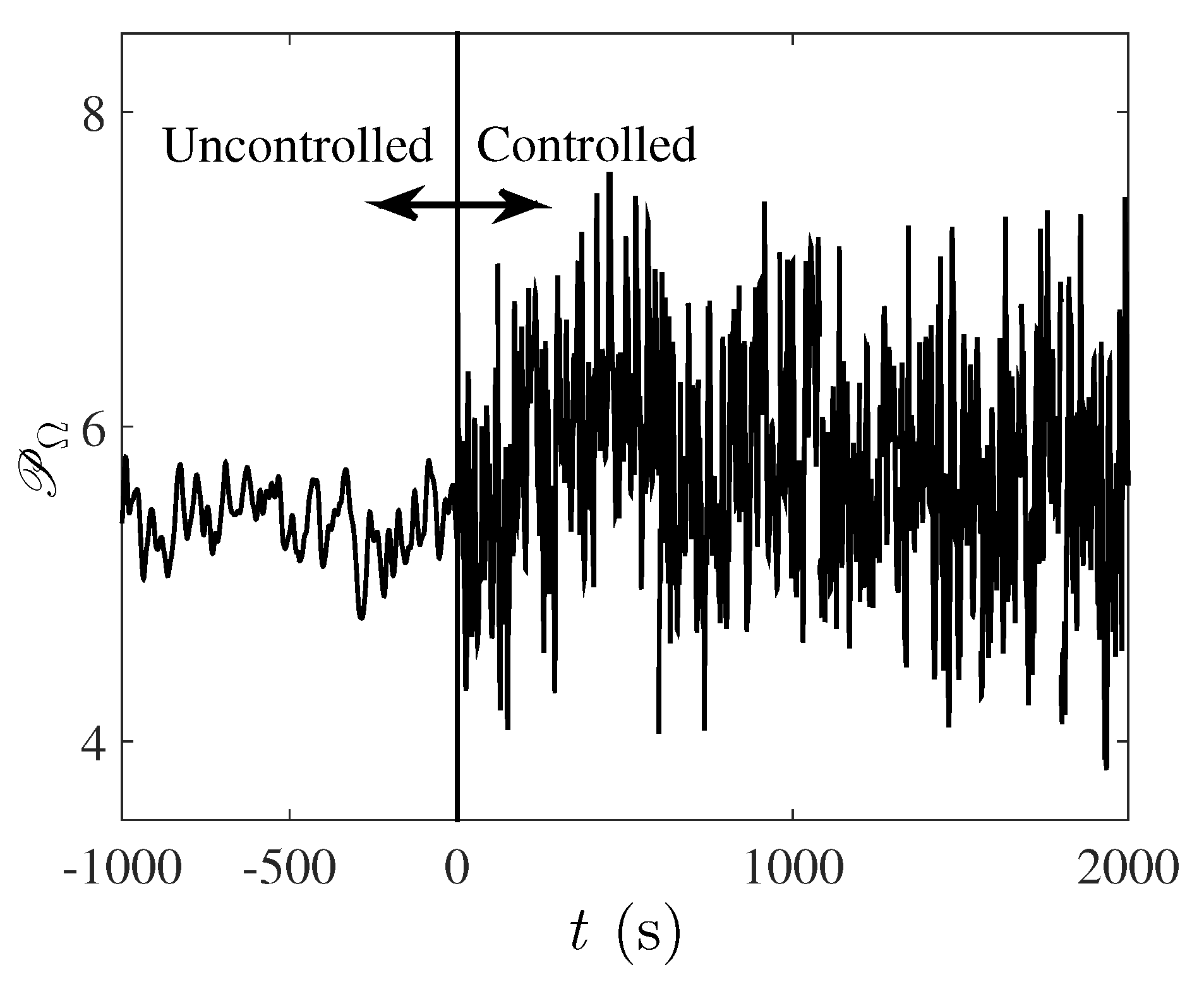
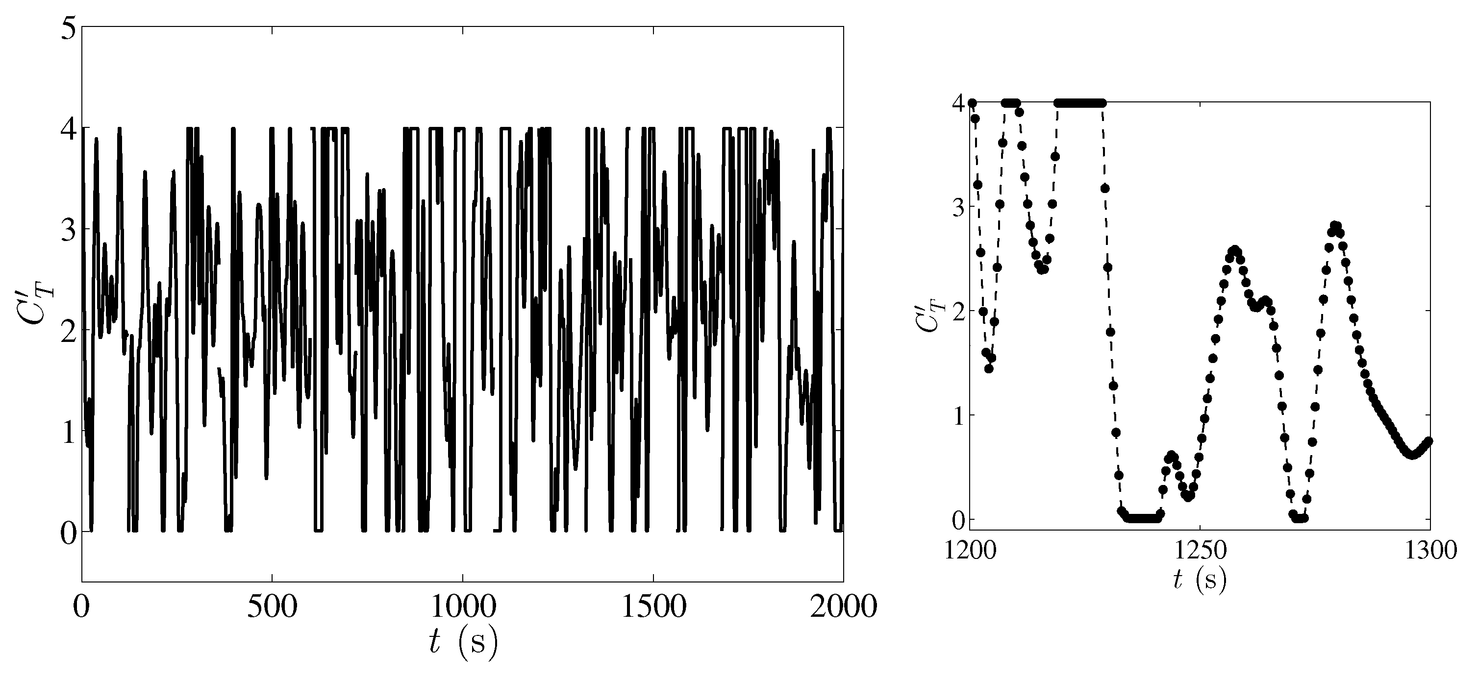
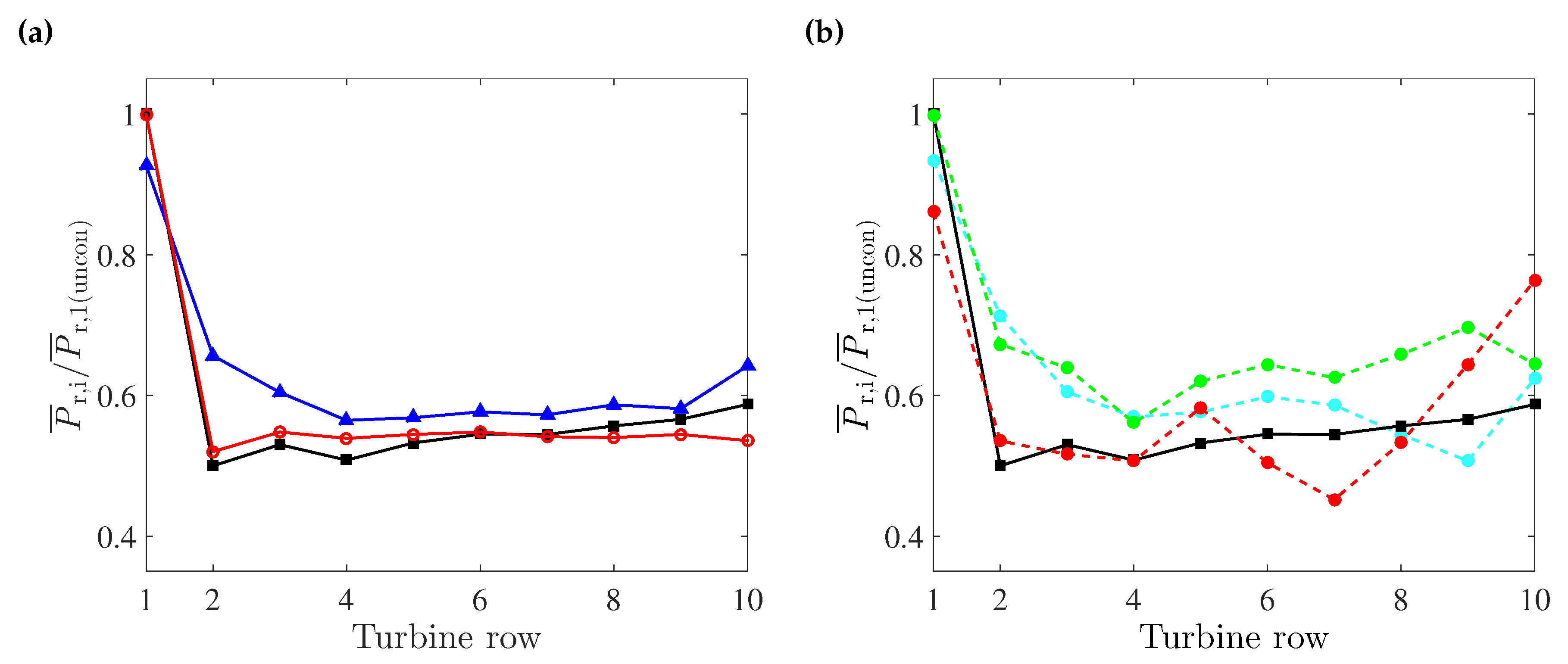
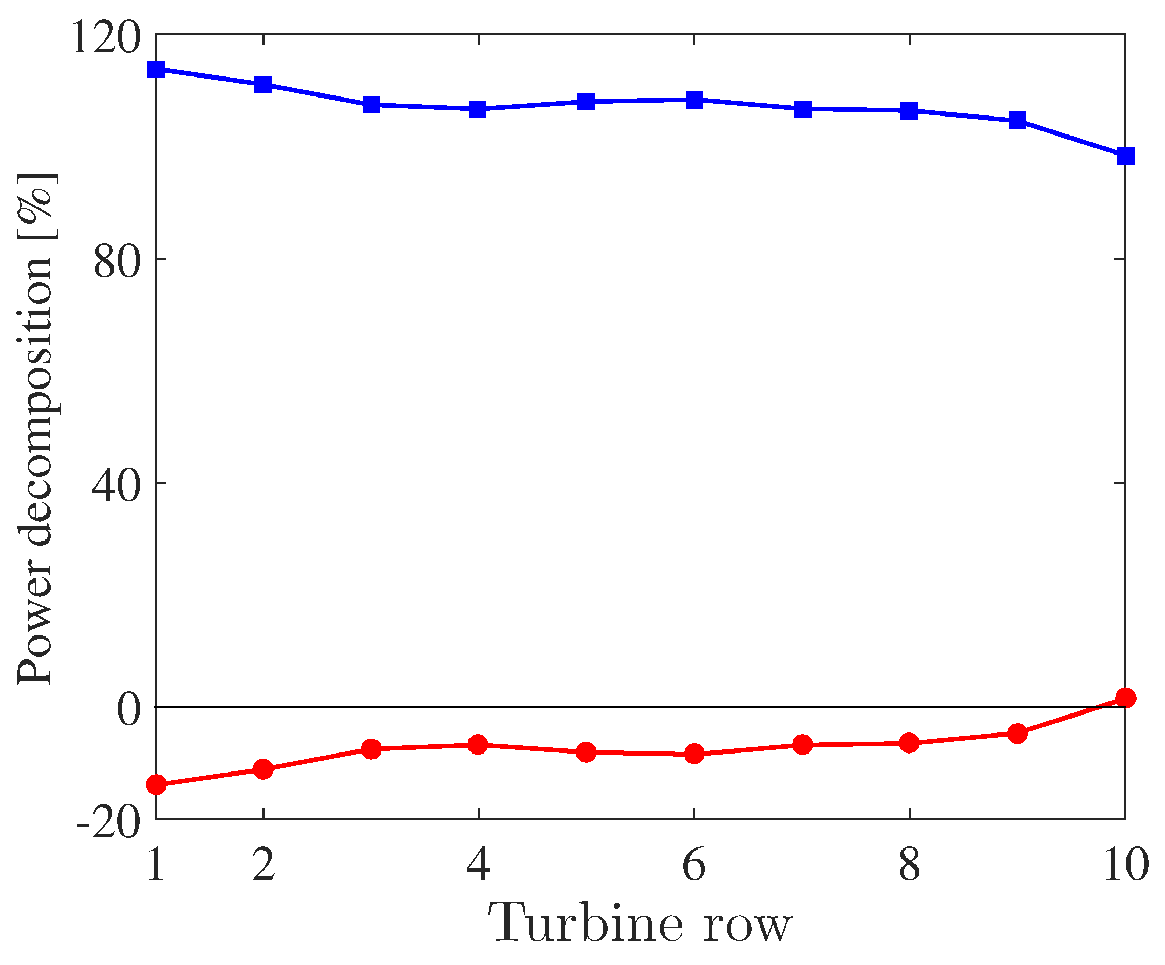
3.1. Controls and Optimized Power Output

First of all, in Figure 5, a time series of the total wind farm power extraction per unit farm area is shown, choosing the time origin t = 0 s as the point where the optimal control is started. For 1000 s t < 0 s, all turbines operate in greedy mode with C T , i = 2 . 0 (denoted as the ‘uncontrolled’ case). It is appreciated from the figure that the total farm power fluctuates significantly more after the start of the optimal control. This was also observed in the optimization of the infinite farm. As discussed further below, the increased variability results from the fluctuations of C T , i . When averaging the farm power output over the 2000 s of accumulated optimal control and comparing to the average power output of the uncontrolled case, a gain in energy extraction of 7% is achieved. This value is significantly lower than the gain of 16% in the infinite farm case [3], but a gain of this magnitude is still important. The difference between the finite and infinite case is further discussed below, but one obvious contribution is that the first row of turbines in the developing case is already operating optimally at C T , i = 2 . 0 . In the current farm, the power extraction from the first row accounts for about 17% of the total farm power (in the uncontrolled case).
Figure 4. Contours of instantaneous streamwise adjoint fields, obtained from the first gradient calculation in Control Window 1. Horizontal planes in the figures are taken at the hub height. (a) T t = 22 s; (b) T t = 70 s; (c) T t = 175 s.
Energies 09 00029 g004
Figure 5. Time evolution of total farm power output. At time t = 0 s, optimal control is activated.
Energies 09 00029 g005
In Figure 6, the time evolution of the optimal thrust coefficient for one of the turbines is shown. The control changes strongly in response to the turbulent flow field. It can be seen that C T frequently touches the lower and upper limits imposed by the box constraints, i.e., 0 C T , i ( t ) 4 . When zooming in on C T in Figure 6, it is however appreciated that the control is smoothly represented on the time grid (this is not a priori guaranteed in optimal control problems, often requiring additional regularization). Moreover, the fastest time scale with which C T changes from its lowest to highest value remains above 10 s. Thus, these control actions on C T are not too fast to realize using blade pitching. We should notice here that the current optimal controls may lead to increased structural loading and fatigue. These issues are currently not taken into account in the optimization cost functional. Taking such a detailed structural analysis into account is not in the scope of the current study. This will need further investigation in the future.
Figure 6. Time evolution of the thrust coefficient of one of the turbines in the farm.
Energies 09 00029 g006
In Figure 7, the time-averaged and row-averaged power output of different turbine rows are shown for both the optimal control and uncontrolled cases. All results are normalized by the average power output of the first row in the uncontrolled case. As a further reference, we have also included results from another (uncontrolled) LES of a similar wind farm by Porté-Agel et al. [20]. It is appreciated that the uncontrolled power outputs from the current study largely follow the trend observed by Porté-Agel et al. The uncontrolled power outputs also show a good agreement with typical field data [1,2], as well as with other LES investigations (see, e.g., [43]) of wind farms with similar configurations. A sharp drop in power production is observed between the first row and the second row. For turbine rows further downstream, the power deficit remains more or less constant.
Figure 7. Comparison of the time-averaged power output for the controlled and uncontrolled farm as a function of turbine row. (): power output for the uncontrolled case averaged over the time interval [ 0 , 17 T A ] . (a) ( ) Power output from a prior large eddy simulation (LES) investigation with similar turbine spacing [20]; ( ) comparison to optimal control results averaged over [ 0 , 17 T A ] ; (b) Power output for different control windows. Window 1 ( ); Window 5 ( ); Window 12 ( ).
Energies 09 00029 g007
When looking at the optimal control results in Figure 7a, it is apparent that this typical trend changes. First of all, the power output from the first row is a bit lower compared to the uncontrolled case. However, for the later rows, the power output is significantly higher, and the transition towards a roughly constant power deficit in later rows is much smoother. Figure 7b presents power output averaged over three different control windows (instead of over the full set of 17 windows). A strong variation in the extracted power is observed from window to window, indicating that the control also depends on instantaneous turbulent flow features and that sufficient averaging over a range of control windows is required to accumulate converged statistics.
From Figure 7, it is clear that the power output in Rows 2 to 10 increases significantly. Overall, the power extraction in these rows is increased by 9.6%. The power output of the first row is decreased by about 7.7%. However, in contrast to the optimization of static turbine set-points [9], in the current dynamic optimal control study, this reduction in the first row is more than compensated by the gains in the later rows.

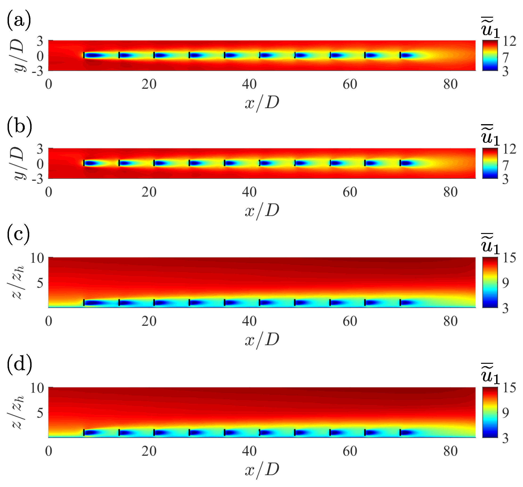
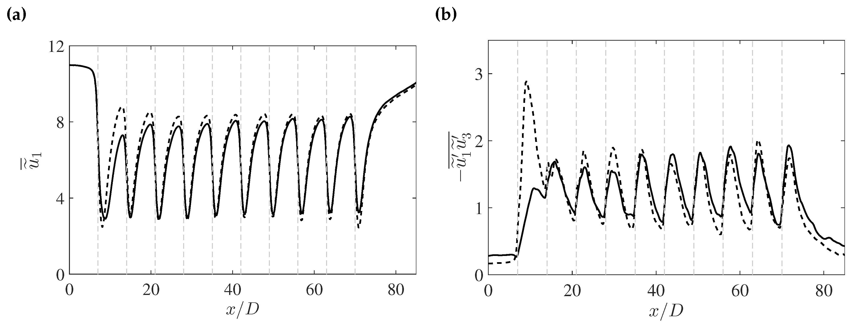
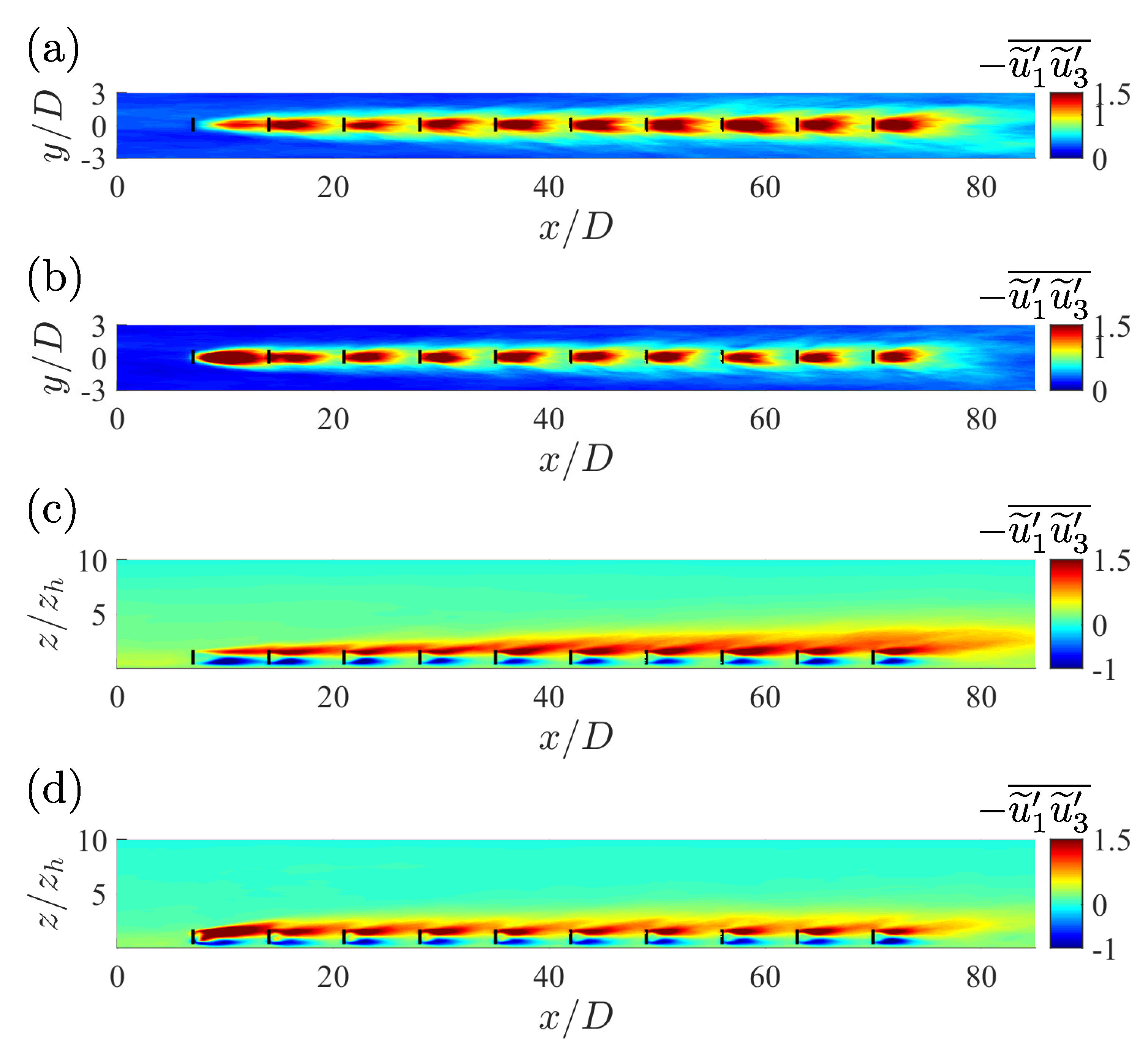
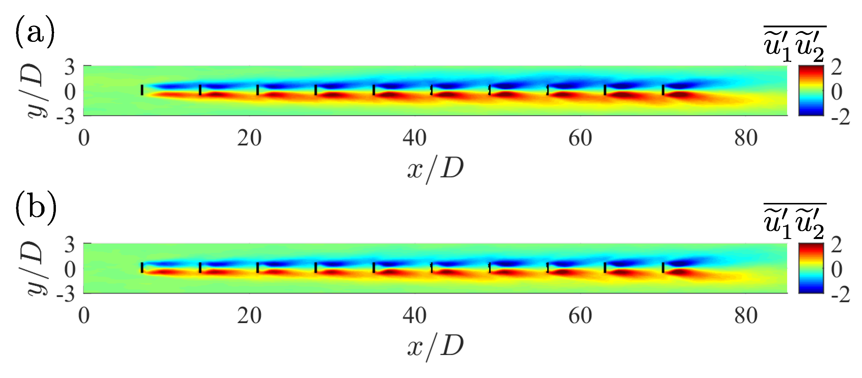
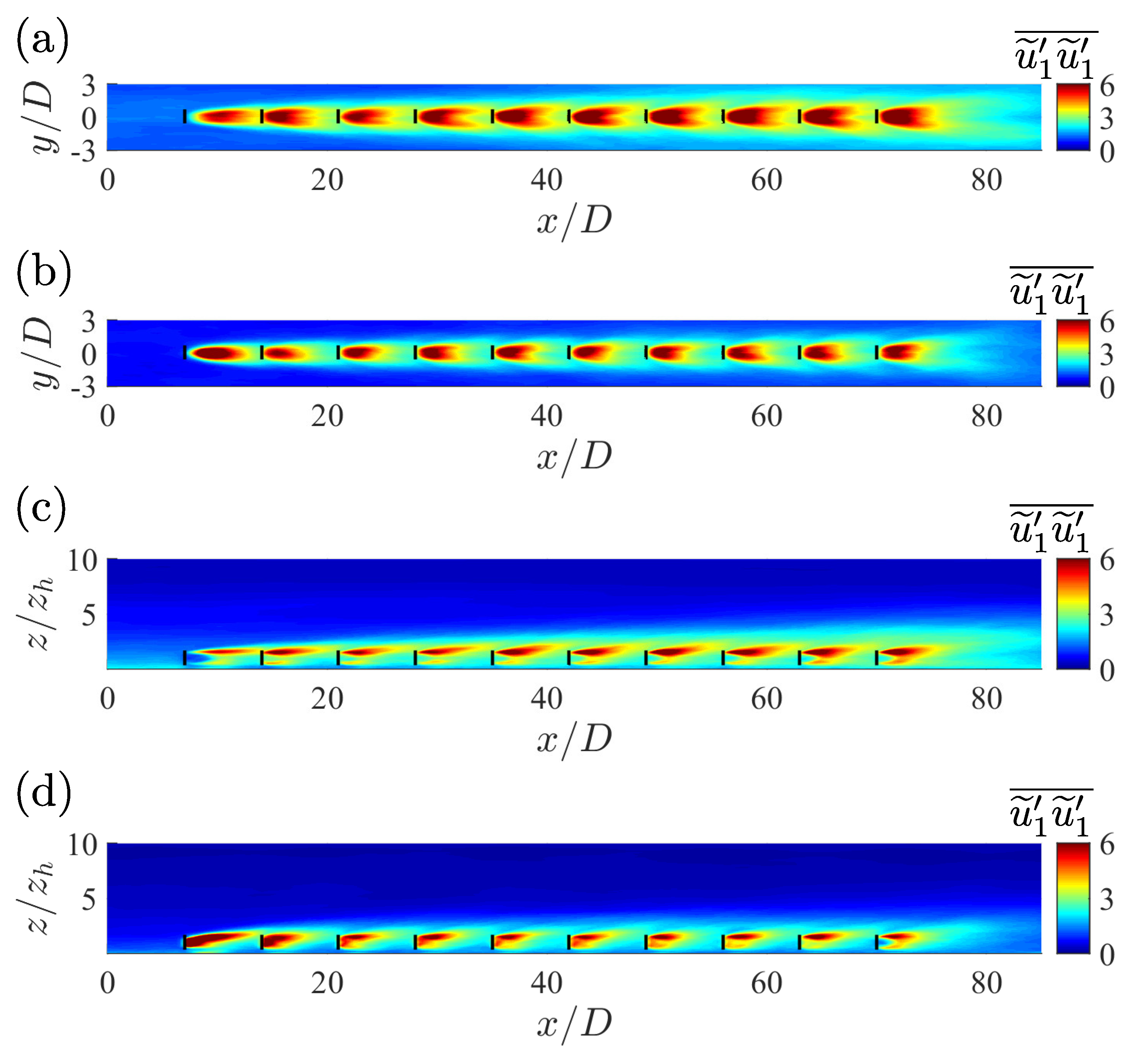
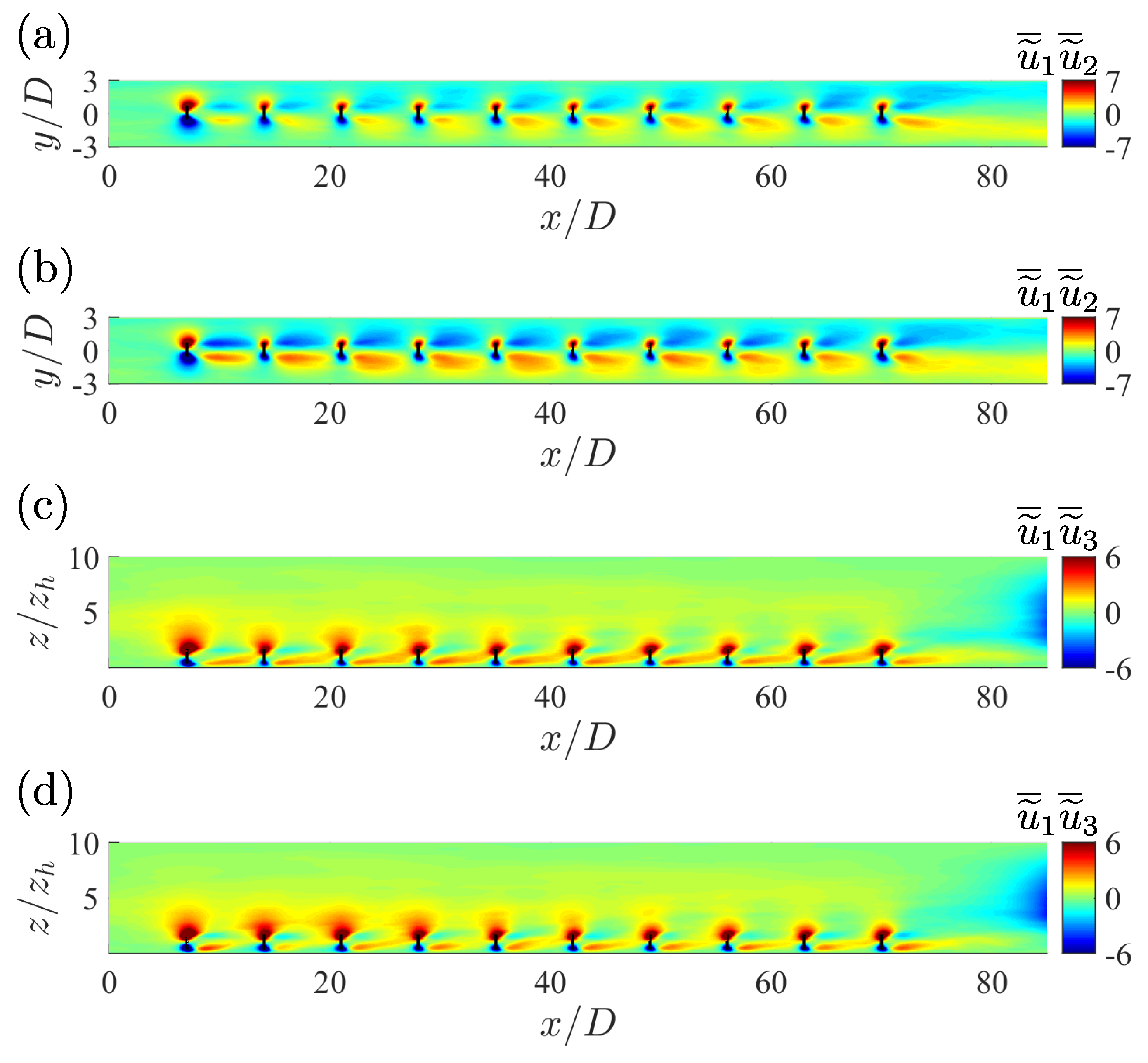
3.2. Averaged Flow Statistics

In order to further understand the relation between the flow field and the power production of the farm, the spatial distributions of the time-averaged mean velocity profiles and Reynolds stresses are analyzed in this subsection. The flow fields of both the uncontrolled case and the optimal control case are averaged over time window [ 0 , 17 T A ] . First of all, in Figure 8a,b, the mean streamwise velocity in a horizontal plane at hub height is shown. Since results are roughly invariant in the spanwise direction (except for small deviations in the two side columns), we also average the flow field of the different turbine columns, including the side rows, showing only one (averaged) column in the plots. Overall, the velocity distribution in the controlled and uncontrolled cases is the same, but distinct differences are observed in the turbine wakes. In the controlled case, most turbine rows have shorter wakes, and this is particularly true for the first row. This is also observed in Figure 8c,d, where the streamwise velocity is shown in an x z -plane through the turbines. Overall, this behavior is quite similar to the observations for the fully-developed wind farm in [3], where the increased energy extraction was also related to improved wake recovery.
Figure 8. Contours of the mean streamwise velocity field averaged over the time window and five columns. (a,b) In a horizontal plane at hub height; (c,d) in a vertical plane through the turbine turbine. (a,c) Uncontrolled case; (b,d) optimal control case.
Energies 09 00029 g008
In Figure 9a, the turbine centerline velocity through the wind farm is shown, also illustrating the better wake recovery and higher inflow velocity of the turbines for the controlled case. Figure 9b shows the accompanying vertical Reynolds shear stress u ˜ 1 u ˜ 3 ¯ at the turbine tip level. For the infinite case in [3], the improved wake recovery of the turbine wakes was related to increased vertical Reynolds stresses in the wake regions. Here, we also observe a significant increase in vertical Reynolds stress after the first turbine row, explaining the faster wake recovery of the first wake. However, at downstream turbine rows, this increased Reynolds stress is not consistently observed in all wakes.
In Figure 10 and Figure 11, the vertical u ˜ 1 u ˜ 3 ¯ and horizontal u ˜ 1 u ˜ 2 ¯ Reynolds shear stresses are shown in more detail in the vertical and horizontal planes. Apart from the wake of the first row, the vertical Reynolds shear stresses are not significantly higher in the controlled case and often even slightly lower than in the uncontrolled case. Moreover, the horizontal Reynolds shear stresses, responsible for sideways exchange of momentum, are not changed at all by the optimal control (also not in the first row). This clearly indicates that some of the mechanisms that increase energy extraction in the farm are not fully equivalent to those observed for the infinite case.
Figure 9. Time and column averaged profiles of (a) streamwise velocity through the rotor center and (b) Reynolds shear stress through the turbine tip. (, black) uncontrolled case; (---, dashed) optimal control case averaged over the time interval [ 0 , 17 T A ] . Vertical dashed lines (light grey) represent the location of the turbines.
Energies 09 00029 g009
Figure 10. Contours of Reynolds shear stress ( u ˜ 1 u ˜ 3 ¯ ) averaged over the time window and five columns. (a,b) In a horizontal plane at the turbine-tip level; (c,d) in a vertical plane through the turbine. (a,c) Uncontrolled case; (b,d) optimal control case.
Energies 09 00029 g010
Figure 11. Contours of Reynolds shear stress ( u ˜ 1 u ˜ 2 ¯ ) averaged over the time window and five columns in a horizontal plane at the hub level. (a) Uncontrolled case; (b) optimal control case.
Energies 09 00029 g011
Looking at the streamwise normal Reynolds stresses u ˜ 1 u ˜ 1 ¯ in Figure 12, it is observed that streamwise velocity fluctuations are even reduced in the controlled case, e.g., leading to less turbulent inflow at the next turbine row. In fact, this is similar to the trends observed for the streamwise Reynolds stresses in the infinite wind farm in [3]. This reduction in inflow turbulence at the next rows is directly related to the faster wake recovery observed above.
Figure 12. Contours of the mean streamwise component of the normal Reynolds stresses averaged over the time window and five columns. (a,b) In a horizontal plane at the turbine-tip level; (c,d) in a vertical plane through the turbine. (a,c) Uncontrolled case; (b,d) optimal control case.
Energies 09 00029 g012
In Figure 13, we investigate the mean transport of momentum around the wind turbines in the controlled and uncontrolled cases. The sideways mean transport u ˜ ¯ 1 u ˜ ¯ 2 is shown in a horizontal plane through the turbine hub in Figure 13a,b, and the vertical transport u ˜ ¯ 1 u ˜ ¯ 3 is shown in a vertical plane in Figure 13c,d. It is observed that mainly the horizontal sideways mean transport is significantly influenced by the optimal control, i.e., the sideways transport is much bigger in the controlled case. The vertical transport remains largely unchanged from the uncontrolled to the controlled case. This is in contrast to the results for the infinite case [3], where a significant difference was found in the vertical transport, leading to much larger vertical dispersive stresses in the controlled case. For the infinite wind farm boundary layer, this is not unexpected, as all energy extracted by the turbines is balanced by vertical transport. A spatially-developing wind farm boundary layer is characterized by unattenuated high energy winds upstream of the wind farm. Given the current arrangement of turbines, a considerable fraction of this energy remains uncaptured by the front row of turbines and, hence, passes between the turbine columns (see, e.g., Figure 2). Thus, in this case, optimal control can gain a lot more from sideways transport, as long as the inflow energy is not yet depleted.
Figure 13. Contours of mean transport terms averaged over the time window and five columns. (a,b) u ˜ ¯ 1 u ˜ ¯ 2 in a horizontal plane at the hub level; (c,d) u ˜ ¯ 1 u ˜ ¯ 3 in a vertical plane through the turbine. (a,c) Uncontrolled case; (b,d) optimal control case.
Energies 09 00029 g013
For the fully-developed case, the increase in turbulence levels in the turbine wakes was attributed to a slight anticorrelation between the control signal C T and the turbine wind velocity [3]. Here, we perform the same analysis, and we expect similar findings for at least the first row of turbines. To that end, a Reynolds decomposition of the power output (cf. Equation (8)) is performed. We decompose the control in its time mean and fluctuating part, i.e., C T , i C T , i ¯ + Δ [ C T , i ] . Similarly, the cubed velocity V ^ i 2 V i is decomposed as V ^ i 2 V i V ^ i 2 V i ¯ + Δ [ V ^ i 2 V i ] . Thus,
P r ¯ = i = 1 N r 1 2 C T , i ¯ V ^ i 2 V i ¯ A + i = 1 N r 1 2 Δ [ C T , i ] Δ [ V ^ i 2 V i ] ¯ A ,
where P r ¯ is the time average of the total power output from a turbine row and N r is the number of turbines in the row. It is obvious that the second term on the right-hand side is zero in the uncontrolled case, since C T is constant in that case, so that Δ [ C T , i ] = 0 .
Figure 14 shows the fraction of the mean and the fluctuating terms on the right-hand side of Equation (14) to the time-averaged total extracted power P r ¯ . It is appreciated that for all but the last row, C T is anticorrelated with V ^ i 2 V i , leading to a negative value for the second term. For the last row, this is no longer the case, as the downstream development of the flow after the last row of turbines does not affect overall power output. For the first row of turbines, the negative correlation is approximately 14% of P r ¯ . This is much higher than the 6% observed in the fully-developed case [3]. Similar to the infinite case, this leads to higher Reynolds stresses and better wake mixing in the wake of the first row. For the latter rows, the negative correlation decreases to about 7%. However, as observed above, this does not directly lead to increased turbulence levels in the wake, but rather to increased sideways inflow of mean momentum. This points to more intricate correlations between C T and the velocity field, e.g., related to the passing of high-speed streaks in the channels between the turbines. Unfortunately, these correlations are difficult to identify. We expect them to be low, as most of the time, turbines still have to extract energy. In addition, it would also be interesting to investigate the correlations between controls from different turbines, as well as the correlations of power output and thrust coefficients with flow events. However, given the current optimal control time span (approximately 2000 seconds), the noise levels of the statistical averages remain too high to find significant correlations. Ongoing work is focusing on improving the parallelization of the adjoint equations and the speed-up of our optimization algorithms [45,46], so that in the future, longer time averaging becomes possible.
Figure 14. Reynolds decomposition of power output from different turbine rows. ( ) Ratio of the mean component to the time-averaged total extracted power; ( ) ratio of the fluctuating component due to C T to the total extracted power.
Energies 09 00029 g014

4. Conclusions

In the current paper, the application of optimal coordinated control was investigated for a finite-sized wind farm in large eddy simulations, extending the work of Goit and Meyers [3] to a regime where entrance effects are important. A receding horizon optimal control framework was considered, and optimization was performed using a gradient-based approach with adjoint simulations for the determination of the gradients. Based on this approach, the energy extraction of turbines was dynamically controlled in time so as to optimally influence the flow field in the boundary layer. Overall, an increase in energy extraction of 7% was achieved by the optimal control. The power output in the first row was a bit lower compared to the uncontrolled case, but this was compensated by increased power output in later rows. Thus, in contrast to the optimization of static turbine set-points where the loss of power in the first row is not recaptured at later rows [9], dynamic optimal control of turbine set-points allows for an overall increase of energy extraction in the farm. Note that for the infinite case, a gain of 16% was reported [3], which is significantly higher than the 7% obtained for the finite case. The difference is attributed to the fact that in the developing case, the first row of turbines, which covers a significant part of the total power output, is already operating optimally, and hence, its performance cannot be further improved.
The improved power extraction in the optimal control regime was shown to be related to improved wake recovery in all turbine rows, leading to higher inflow velocities for individual turbines. However, the mechanisms influencing this wake recovery were different for the first and subsequent rows. In the first row, the vertical Reynolds shear stresses were significantly increased, leading to better mixing from high-speed air above the farm into the wake. For the latter rows, neither Reynolds shear stresses nor vertical transport of momentum were significantly affected. Instead, sideways mean transport of momentum from high-speed channels in between turbines towards the wake regions was significantly increased.
The current study considered an aligned wind farm under neutral atmospheric conditions and further included a number of specific choices on turbine spacing, the admissible range for the controls C T ( t ) , the control time window, the number of iterations in the conjugate gradient method, etc. In further research, it will be interesting to look at other arrangement patterns, effects of stratification, larger wind farms and different constraints on the controls. Moreover, by improving the parallelism of the adjoint code and the efficiency of optimization algorithms, averaging over longer time periods will become feasible, so that a more detailed analysis of the correlations between controls and flow events becomes possible. It will also be interesting to compare current results with the optimal control using more advanced turbine representations, such as an actuator line model (ALM). In particular, when evolving computational resources allow wind farm optimal control with finer grids, an ALM inserts much more detailed near-wake physics into the flow, such as, e.g., tip vortices. Moreover, a more realistic representation of the turbine control through generator torque and blade pitching is then also possible. Nowadays, such an approach would already be feasible for smaller domains, e.g., focusing on one or two turbines, though it would still require the formulation of the adjoint actuator line model. This is the subject of ongoing research.

Acknowledgments

The authors acknowledge support from the European Research Council (FP7-Ideas, Grant No. 306471), the Flemish Science Foundation (FWO, Grant No. G.0376.12), and BOF KU Leuven (Grant No. IDO/11/012). Simulations were performed on the computing infrastructure of the VSC (Flemish Supercomputer Center), funded by the Hercules Foundation and the Flemish Government.

Author Contributions

Jay P. Goit and Johan Meyers jointly set up the study and wrote the manuscript. Jay P. Goit performed all simulations and implementations. Wim Munters implemented the fringe-region technique allowing non-periodic simulations in SP-Wind and assisted in final copy editing of the manuscript.

Conflicts of Interest

The authors declare no conflict of interest.

References

  1. Barthelmie, R.; Rathmann, O.; Frandsen, S.T.; Hansen, K.; Politis, E.; Prospathopoulos, J.; Rados, K.; Cabezón, D.; Schlez, W.; Phillips, J.; et al. Modelling and measurements of wakes in large wind farms. J. Phys.: Conf. Ser. 2007, 75, 012049. [Google Scholar] [CrossRef]
  2. Barthelmie, R.; Pryor, S.; Frandsen, S.; Hansen, K.; Schepers, J.G.; Rados, K.; Schlez, W.; Neubert, A.; Jensen, L.E.; Neckelmann, S.; et al. Quantifying the impact of wind turbine wakes on power output at offshore wind farms. J. Atmos. Ocean. Technol. 2010, 27, 1302–1317. [Google Scholar] [CrossRef]
  3. Goit, J.P.; Meyers, J. Optimal control of energy extraction in wind farm boundary layers. J. Fluid Mech. 2015, 768, 5–50. [Google Scholar] [CrossRef] [Green Version]
  4. Steinbuch, M.; de Boer, W.W.; Bosgra, O.H.; Peters, S.; Ploeg, J. Optimal control of wind power plants. J. Wind Eng. Ind. Aerodyn. 1988, 27, 237–246. [Google Scholar] [CrossRef]
  5. Johnson, K.E.; Thomas, N. Wind farm control: Addressing the aerodynamic interaction among wind turbines. In Proceedings of the American Control Conference (ACC ’09), St. Louis, MO, USA, 10–12 June 2009; pp. 2104–2109.
  6. Horvat, T.; Spudic, V.; Baotic, M. Quasi-stationary optimal control for wind farm with closely spaced turbines. In Proceedings of the 35th International Convention (MIPRO Croatian Society), Opatija, Croatia, 21–25 May 2012; pp. 829–834.
  7. Soleimanzadeh, M.; Wisniewski, R.; Kanev, S. An optimization framework for load and power distribution in wind farms. J. Wind Eng. Ind. Aerodyn. 2012, 107–108, 256–262. [Google Scholar] [CrossRef]
  8. Knudsen, T.; Bak, T.; Svenstrup, M. Survey of wind farm control–power and fatigue optimization. Wind Energy 2014, 8, 1333–1351. [Google Scholar] [CrossRef]
  9. Gebraad, P.M.O. Data-driven Wind Plant Control. Ph.D. Thesis, Delft University of Technology, Delft, The Netherlands, 2014. [Google Scholar]
  10. Park, P.; Holm, R.; Medici, D. The application of PIV to the wake of a wind turbine in yaw. In Proceedings of the 4th International Symposium on Particle Image Velocimetry, Gottingen, Germany, 17–19 September 2001.
  11. Fleming, P.A.; Gebraad, P.M.; Lee, S.; van Wingerden, J.W.; Johnson, K.; Churchfield, M.; Michalakes, J.; Spalart, P.; Moriarty, P. Evaluating techniques for redirecting turbine wakes using SOWFA. Renew. Energy 2014, 70, 211–218. [Google Scholar] [CrossRef]
  12. Gebraad, P.M.O.; Teeuwisse, F.W.; van Wingerden, J.W.; Fleming, P.A.; Ruben, S.D.; Marden, J.R.; Pao, L.Y. Wind plant power optimization through yaw control using a parametric model for wake effects-a CFD simulation study. Wind Energy 2014, 1822, 1–20. [Google Scholar] [CrossRef]
  13. Hansen, A.D.; Sørensen, P.; Iov, F.; Blaabjerg, F. Centralised power control of wind farm with doubly fed induction generators. Renew. Energy 2006, 31, 935–951. [Google Scholar] [CrossRef]
  14. Soleimanzadeh, M.; Wisniewski, R.; Johnson, K. A distributed optimization framework for windfarms. J. Wind Eng. Ind. Aerodyn. 2013, 123, 88–98. [Google Scholar] [CrossRef]
  15. Yang, Z.; Li, Y.; Seem, Y. Maximizing wind farm energy capture via nested-loop extremum seeking control. In Proceedings of the ASME Dynamic Systems and Control Conference, Palo Alto, CA, USA, 21–23 October 2013.
  16. Marden, J.R.; Ruben, S.D.; Pao, L.Y. A model-free approach to wind farm control using game theoretic methods. IEEE Trans. Control Syst. Technol. 2013, 21, 1207–1214. [Google Scholar] [CrossRef]
  17. Gebraad, P.M.O.; van Wingerden, J.W. Maximum power-point tracking control for wind farms. Wind Energy 2014, 18, 429–447. [Google Scholar] [CrossRef]
  18. Ahmad, M.A.; Azuma, S.; Sugie, T. A model-free approach for maximizing power production of wind farm using multi-resolution simultaneous perturbation stochastic approximation. Energies 2014, 7, 5624–5646. [Google Scholar] [CrossRef] [Green Version]
  19. Katić, I.; Hojstrup, J.; Jensen, N.O. A Simple Model for Cluster Efficiency; European Wind Energy Association Conference and Exhibition: Rome, Italy, 1986; pp. 407–410. [Google Scholar]
  20. Porté-Agel, F.; Wu, Y.; Chen, C. A numerical study of the effects of wind direction on turbine wakes and power losses in a large wind farm. Energies 2013, 6, 5297–5313. [Google Scholar] [CrossRef]
  21. Stevens, R.J.A.M.; Gayme, D.F.; Meneveau, C. Effects of turbine spacing on the power output of extended wind farms. Wind Energy 2016, in press. [Google Scholar] [CrossRef]
  22. Abkar, M.; Porté-Agel, F. Influence of atmospheric stability on wind-turbine wakes: A large-eddy simulation study. Phys. Fluids 2015, 27, 035104. [Google Scholar] [CrossRef]
  23. Abkar, M.; Porté-Agel, F. The effect of free-atmosphere stratification on boundary-layer flow and power output from very large wind farms. Energies 2013, 6, 2338–2361. [Google Scholar] [CrossRef]
  24. Allaerts, D.; Meyers, J. Large eddy simulation of a large wind-turbine array in a conventionally neutral atmospheric boundary layer. Phys. Fluids 2015, 27, 065108. [Google Scholar] [CrossRef]
  25. Meyers, J.; Sagaut, P. Evaluation of smagorinsky variants in large-eddy simulations of wall-resolved plane channel flows. Phys. Fluids 2007, 19, 095105. [Google Scholar] [CrossRef] [Green Version]
  26. Delport, S.; Baelmans, M.; Meyers, J. Constrained optimization of turbulent mixing-layer evolution. J. Turbul. 2009, 10, 1–26. [Google Scholar] [CrossRef]
  27. Meyers, J.; Meneveau, C. Large eddy simulations of large wind-turbine arrays in the atmospheric boundary layer. In Proceedings of the 48th AIAA Aerospace Sciences Meeting Including the New Horizons Forum and Aerospace Exposition, Orlando, FL, USA, 4–7 January 2010; pp. 1–10.
  28. Smagorinsky, J. General circulation experiments with the primitive equations: I. The basic experiment. Mon. Weather Rev. 1963, 91, 99–165. [Google Scholar] [CrossRef]
  29. Mason, P.J.; Thomson, T.J. Stochastic backscatter in large-eddy simulations of boundary layers. J. Fluid Mech. 1992, 242, 51–78. [Google Scholar] [CrossRef]
  30. Calaf, M.; Meneveau, C.; Meyers, J. Large eddy simulation study of fully developed wind-turbine array boundary layers. Phys. Fluids 2010, 22, 015110. [Google Scholar] [CrossRef]
  31. Martinez Tossas, L.A.; Leonardi, S.; Moriarty, P. Wind Turbine Modeling for Computational Fluid Dynamics; NREL Technical Report SR-5000-55054; National Renewable Energy Laboratory (NREL): Golden, CO, USA, 2013.
  32. Wu, Y.-T.; Porté-Agel, F. Large-eddy simulation of wind-turbine wakes: Evaluation of turbine parametrisations. Bound.-Layer Meteorol. 2011, 138, 345–366. [Google Scholar] [CrossRef]
  33. Moeng, C.H. A large-eddy simulation model for the study of planetary boundary-layer turbulence. J. Atmos. Sci. 1984, 41, 2052–2062. [Google Scholar] [CrossRef]
  34. Bou-Zeid, E.; Meneveau, C.; Parlange, M.B. A scale-dependent Lagrangian dynamic model for large eddy simulation of complex turbulent flows. Phys. Fluids 2005, 17, 025105. [Google Scholar] [CrossRef]
  35. Spalart, P.R. Direct numerical study of leading edge contamination. In AGARD Conference Proceedings, Fluid Dynamics of Three-Dimensional Turbulent Shear Flows and Transition; Advisory Group for Aerospace Research and Development (AGARD): Neuilly-sur-Seine, France, 1988; Volume 438, pp. 5.1–5.13. [Google Scholar]
  36. Canuto, C.; Hussaini, M.Y.; Quarteroni, A.; Zang, T.A. Spectral Methods: Evolution to Complex Geometries and Application to Fluid Dynamics; Springer: Berlin, Germany, 2007. [Google Scholar]
  37. Verstappen, R.W.C.P.; Veldman, A.E.P. Symmetry-preserving discretization of turbulent flow. J. Comput. Phys. 2003, 187, 343–368. [Google Scholar] [CrossRef]
  38. Press, W.H.; Teukolsky, S.A.; Vetterling, W.T.; Flannery, B.P. Numerical Recipes in FORTRAN77: The Art of Scientific Computing, 2nd ed.; Cambridge University Press: Cambridge, UK, 1996. [Google Scholar]
  39. Luenberger, D.G. Linear and Nonlinear Programming, 2nd ed.; Kluwer Academic Publishers: Boston, MA, USA, 2005. [Google Scholar]
  40. Nocedal, J.; Wright, S.J. Numerical Optimization, 2nd ed.; Springer: Berlin, Germany, 2006. [Google Scholar]
  41. Choi, H.; Hinze, M.; Kunisch, K. Instantaneous control of backward-facing step flows. Appl. Numer. Math. 1999, 31, 133–158. [Google Scholar] [CrossRef]
  42. Meyers, J.; Meneveau, C. Flow visualization using momentum and energy transport tubes and applications to turbulent flow in wind farms. J. Fluid Mech. 2013, 715, 335–358. [Google Scholar] [CrossRef] [Green Version]
  43. Stevens, R.J.A.M.; Graham, J.; Meneveau, C. A concurrent precursor inflow method for Large Eddy Simulations and applications to finite length wind farms. Renew. Energy 2014, 68, 46–50. [Google Scholar] [CrossRef]
  44. Jonkman, J.; Butterfield, S.; Musial, W.; Scott, G. Definition of a 5-MW Reference Wind Turbine for Offshore System Development; NREL Technical Report TP-500-38060; National Renewable Energy Laboratory (NREL): Golden, CO, USA, 2009.
  45. Badreddine, H.; Vandewalle, S.; Meyers, J. Sequential quadratic programming (SQP) for optimal control in direct numerical simulation of turbulent flow. J. Comput. Phys. 2014, 256, 1–16. [Google Scholar] [CrossRef] [Green Version]
  46. Nita, C.; Vandewalle, S.; Meyers, J. On the efficiency of gradient based optimization algorithms for DNS-based optimal control in a turbulent channel flow. Comput. Fluids 2015, 125, 11–24. [Google Scholar] [CrossRef]

